Evaluating Global Reanalysis Datasets as Input for Hydrological Modelling in the Sudano-Sahel Region

Abstract

This paper investigates the potential of using global reanalysis datasets as input for hydrological modelling in the data-scarce Sudano-Sahel region. To achieve this, we used two global atmospheric reanalyses (Climate Forecasting System Reanalysis and European Center for Medium-Range Weather Forecasts (ECMWF) ERA-Interim) datasets and one global meteorological forcing dataset WATCH Forcing Data methodology applied to ERA-Interim (WFDEI). These datasets were used to drive the Soil and Water Assessment Tool (SWAT) in the Logone catchment in the Lake Chad basin. Model performance indicators after calibration showed that, at daily and monthly time steps, only WFDEI produced Nash Sutcliff Efficiency (NSE) and Coefficient of Determination (R²) values above 0.50. Despite a general underperformance compared to WFDEI, CFSR performed better than the ERA-Interim. Model uncertainty analysis after calibration showed that more than 60% of all daily and monthly observed streamflow values at all hydrometric stations were bracketed within the 95 percent prediction uncertainty (95PPU) range for all datasets. Results from this study also show significant differences in simulated actual evapotranspiration estimates from the datasets. Overall results showed that biased corrected WFDEI outperformed the two reanalysis datasets; meanwhile CFSR performed better than the ERA-Interim. We conclude that, in the absence of gauged hydro-meteorological data, WFDEI and CFSR could be used for hydrological modelling in data-scarce areas such as the Sudano-Sahel region.

1. Introduction

Long-term and well distributed climate information is essential to enhance water resources management and to guide policies aimed addressing the consequences of climate variability and change from a local to global scale [1]. This data is needed because the quantitative estimation of water balance components is important to understand the variations taking place at catchment/global level [2]. However, in many developing and arid regions of the world, the assessment and management of water resources is still a major challenge due to data scarcity [3]. According to Gorgoglione et al. [4], the difficulty in collecting data in semi-arid and other remote regions can be attributed to several reasons: (i) lack of reliable equipment; (ii) absence of good archiving system and software to store and process the data, and lack of funds to organize data collection campaigns. Another challenge in these regions is that even when data is collected and archived, the effort and money required to access them can be quite substantial [5]. Hydrological models are designed to fill some of these gaps, and their application to enhance water resources management is widely acknowledged [6].

Rainfall is one of the most important inputs used to drive hydrological models; hence it is important to obtain rainfall data of sufficient temporal and spatial resolution. Nevertheless, due to the high spatiotemporal variability of rainfall, it can only be accurately captured by a dense network of rain gauge stations [7]. However, most often, rain gauges may be located outside the area of interest or could exhibit significant gaps in spatial coverage, especially in remote and ungauged areas [5].

Current advances in remote sensing offer many advantages, e.g., satellites observing the Earth have generated potentially useful data that can be used to improve water resources management. Even so, satellite data is usually developed for application in large areas, e.g., at continental or global scale. Therefore, its application at catchment scale for hydrological modelling requires further downscaling, transformation or interpolation which may increase uncertainties in the data [8].

To overcome this challenge, multiyear global gridded representations of weather known as reanalysis datasets are now available. Examples of widely used reanalysis datasets include: National Centers for Environmental Prediction (NCEP)/National Center for Atmospheric Research (NCAR), Climate Forecasting System Reanalysis (CFSR) [9], European Center for Medium-Range Weather Forecasts (ECMWF) ERA-Interim [10] and Modern-Era Retrospective Analysis for Research and Applications (MERRA) [11]. However, it has been shown that significant differences exist in precipitation estimates from these products [12]. Lorenz and Kunstmann [12] assert that the quality of precipitation estimates from reanalyses datasets depends on the geographic location, especially in tropical regions. Furthermore, a recent study by Essou et al. [13] demonstrated that the performance of reanalysis datasets may vary from one climatic zone to another.

To address the issue of bias inherent in reanalysis products; global forcing datasets have been developed using post processing techniques (e.g., bias correction) based on observations [14]. An example of such bias corrected dataset is the WATCH Forcing Data methodology applied to ERA Interim (WFDEI) [14].

Another issue often overlooked in most studies evaluating the performance of reanalysis datasets in hydrologica modelling is the impact of spatial resolution of each dataset on the quality of the simulated streamflow. In fact, the effect of rainfall spatial variability on streamflow and water balance components have been shown to be significant in catchments with high spatial variability [15]. Lobligeois et al. [16] in their study demonstrated the importance of spatial representation in areas subjected to high spatial variability in rainfall. Given that the distance between reanalysis grid points is quasi uniform, these datasets could be used to investigate the impact of rainfall spatial variability on hydrological processes such as streamflow and evapotranspiration in large catchments.

Recently, reanalysis datasets have been used as input for hydrological modelling in many studies with different degrees of successes recorded. For example, Essou et al. [13] used CFSR, ERA-Interim, MERRA and WFDEI as input for streamflow simulation using a conceptual model in several watersheds in the US and concluded that these datasets had good potential to be used for hydrological modelling. Monteiro et al. [17] used CFSR and WFDEI to drive the Soil and Water Assessment Tool (SWAT) for hydrological modelling in the Tocantins catchment in Brazil and asserted that WFDEI outperformed CFSR in their study area. Andersson et al. [18] used ERA-Interim and WFDEI as input to drive the hydrological catchment model (HYPE) in Europe and Africa. They concluded that WFDEI improved streamflow simulation compared to Watch Forcing data methodology applied to ERA-40. Krogh et al. [19] used CFSR and ERA-Interim to drive the Cold Regions Hydrological Model (CRHM) in the upper Baker river basin in Chile and concluded that CFSR simulated streamflow better than ERA-Interim. These numerous studies suggest that reanalysis datasets could be used for hydrological modelling in data scarce regions. Despite widespread hydro-meteorological data scarcity in Africa in general and the Sudano-Sahel region in particular, the use of reanalyses datasets for hydrological modelling in this area remains largely unstudied.

The Logone catchment presents special attributes for the evaluation of reanalysis datasets because it is located at the transition zone between the Sudano and Sahel areas where rainfall is highly variable both in space and time [20]. Furthermore, like most catchments in the region, the Logone suffers from acute observational data scarcity. Given that the performance of reanalysis products in hydrological modelling is largely determined by the quality of the precipitation estimates, Essou et al.; Monteiro et al. and Krogh et al. [13,17,19] recommend that the correlation between observed rainfall and reanalysis precipitation estimates should be assessed before the latter is used as input for hydrological modelling. In a previous study in the catchment, the authors of [21] evaluated the quality of precipitation estimates from CFSR and ERA-Interim against observed monthly rainfall covering the period 1979–2002 and concluded that, precipitation estimates from both reanalyses products could reproduce the seasonal rainfall cycle in the catchment albeit significant variability in the data.

The objectives of this study were; (i) to evaluate the ability of two reanalysis datasets; CFSR and ERA-Interim and one bias corrected global meteorological forcing dataset WFDEI to be used as input to drive the SWAT model in the Logone catchment; and (ii) to evaluate the impact of reanalysis spatial resolution on the quality of simulated flows. This study will be useful in validating the use of reanalysis datasets in data scarce catchments subject to high spatial rainfall variability. In addition, Siam et al. [22] have argued that driving hydrological models with reanalyses datasets to reproduce observed streamflow represents one of the most accurate ways to evaluate how the hydrological cycle is simulated by reanalysis forecast models. Including WFDEI will permit us to assess the impact of bias correction on the performance of ERA-Interim. It is not our intention in this study to judge the quality of each reanalysis dataset or recommend the use of one product over another. This choice depends on personal preference because the performance of each reanalysis product varies from one region to another and one from climatic zone to another as mentioned earlier. A limitation of this study is the absence of daily rain gauge data that could also be used to drive SWAT to compare the performance of the reanalysis datasets against gauge data in simulating streamflow.

2. Materials and Methods

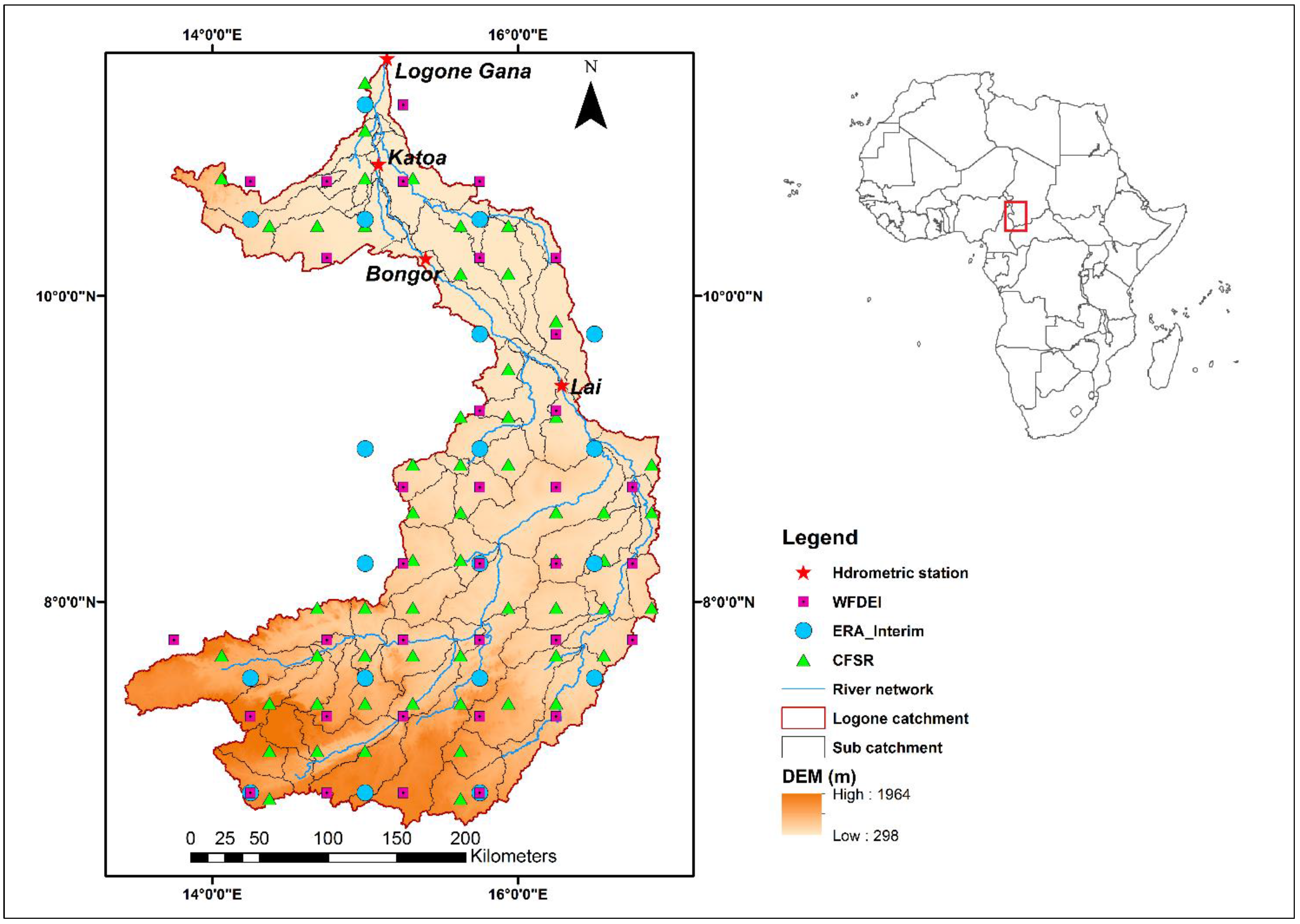
2.1. Study Area

The Logone catchment (Figure 1) is a transnational catchment shared by Cameroon, Chad and Central Africa Republic, with an estimated area of about 86,500 km² lying between latitude 6° and 12° N and longitude 13°–17° E. There are two National Parks in the catchment (Waza and Kalamaloue), with high concentration of wildlife [23]. The Logone River has its source in Cameroon through the Mbere and Vina rivers from the north eastern slopes of the Adamawa Plateau. In Lai, it is joined by the Pende River from Central Africa Republic and flows for about 1000 km in a South-North direction with an elevational range from 300 masl in the north to about 1200 masl in the south. The basin topography, apart from some local mountains in the south is very flat with an average slope of less than 1.3%. The catchment has a semi-arid climate in the north where annual rainfall varies between 600 and 900 mm/year and Sudano climate in the south where annual rainfall varies between 900 and 1400 mm/year. The climate is also characterized by high spatio-temporal variability in rainfall controlled by the oceanic regime from the south and the continental regime from the north [20]. Almost all rain falls during the rainy season from May/June to September/October with high spatial and temporal variability and mean annual temperature is about 28 °C [23].

2.2. Data Sources

2.2.1. Observed River Discharge Data

Daily river discharge measurements were obtained from the Lake Chad Basin Commission (LCBC) covering the period 1983–1997 at four discharge stations. Gaps in the river discharge data were filled using Artificial Neural Networks Self-Organizing Maps (ANN-SOM) [24].

2.2.2. Spatial Datasets

Digital Elevation Model (DEM) data obtained from Shuttle Radar Topographic Mission (SRTM) at a spatial resolution of 90 m was used for catchment delineation. Land cover/use maps were obtained from Climate Change Initiative Land Cover (CCI-LC) at a spatial resolution of 300 m. The land cover was reclassified in the ARCSWAT interface according to model input requirements. Soil data was obtained from the Food and Agricultural Organization (FAO), Harmonize World Soil Database (HWSD) at a spatial resolution of 1 km.

2.2.3. Reanalysis Data

A reanalysis project involves the reprocessing of observational data spanning an extended historical period. “It makes use of a consistent modern analysis system, to produce a dataset, that to a certain extent can be regarded as a “proxy” for observation with the advantage of providing coverage and time resolution often unobtainable with normal observational network” [25]. It is generated with a data assimilation system combining observations with a numerical weather prediction model. For the entire reanalysis period, the model physics remain unchanged in the forecast model for consistency of the output data. The reanalysis consequently provides a physical picture of the global climate over a period during which observational data are available.

2.3. CFSR

The Climate Forecast System, NCEP version 2 is an upgraded version of CFS version one (CFSv1). It was first developed as part of the Climate Forecast System by NCEP in 2004 with quasi-global coverage, fully coupled atmosphere-ocean-land model used by NCEP for seasonal prediction [9]. CFSR has a 3D-variational analysis scheme of the upper-air atmospheric state with 64 vertical levels with a horizontal resolution of 38km spanning the period 1st January 1979 to present day [9].

2.4. ERA-Interim

ERA-Interim is the latest global atmospheric reanalysis produced by the European Centre for Medium-Wave Forecasts (ECMWF) and covers the period from 1 January 1979 to present day [10]. The core component of the ERA-Interim data assimilation system is the 12-h 4D-variational analysis scheme of the upper-air atmospheric state, which is on a spectral grid with triangular truncation of 255 waves (corresponding to approximately 80 km) spatial resolution and a hybrid vertical coordinate system with 60 vertical levels.

2.5. WFDEI

The WATCH Forcing Data methodology applied to ERA-Interim (WFDEI) dataset [14] is produced from Watch Forcing Data (WFD) and ERA-Interim reanalysis via sequential interpolation to a 0.5° resolution, elevation correction and monthly-scale adjustments based on CRU TS3.1/TS3.21 and GPCCv5/v6 monthly precipitation observations for 1979–2012.

Details of the three products can be found in [9,10,14] for CFSR, ERA-Interim and WFDEI respectively. For the Logone catchment, the reanalysis datasets were obtained for an area bounded by latitude 6°–12.0° N and longitude 13°–17.25°E from the Texas A&M University for CFSR, ECMWF for ERA Interim and Lund University for WFDEI. All variables were obtained at a daily time step with spatial resolution of 0.312° (~38 km), 0.50° (~55 km) and 0.75° (~80 km) for CFSR, WFDEI and ERA-Interim respectively hereafter referred to as high, medium and low resolution.

2.6. Model Setup

River discharge at various locations along the Logone River was simulated using the SWAT [26] in the ArcSWAT interface. SWAT is one of the most widely used river basin–scale models worldwide, applied extensively for solving a broad range of hydrologic and environmental problems [26].

In this study, we focus only on water quantity simulation accomplished through two steps: (i) the land phase of the hydrological cycle which controls the amount of water transferred to the main channel from each sub catchment; and (ii) the routing phase which involves the movement of water through the channel network to the outlet. The hydrologic cycle in the land phase of the model is simulated using the water balance equation:

$$S{W}_t=S{W}_0+{\displaystyle \sum }_{i=1}^n(R_{day}-Q_{surf}-E_a-W_{seep}-Q_{gw})$$

(1)

SW_t is the final soil water content (mm), SW₀ is the initial water content (mm), R_day is the amount of precipitation on day i (mm) Q_surf is the amount of surface water runoff on day i (mm), E_a is the amount of actual transpiration on day i (mm), W_seep is the amount of water entering the vadose zone from the soil profile on day I (mm) and Q_gw is the amount of return flow on day i (mm). Details of equations and methods used to estimate various hydrological components can be found in [27]. During model development, SWAT divides a catchment into sub catchments using digital elevation model (DEM) data. The spatial distribution of hydrological processes over each sub catchment is represented through hydrologic response units (HRUs), used to further divide the sub catchments into smaller units. The HRU can be defined as a land area within a sub catchment with the same land use class, soil type, slope class and management combinations.

While building the model, an attempt was made to maximize the number of grid points used for streamflow simulation using CFSR as the reference dataset because of its high spatial resolution (0.312°) compared to the other two. Different threshold areas were tested for catchment delineation. Reducing the threshold area to 500 km² did not increase the number of reanalysis grid points selected while increasing it 1000 km² reduced the number to only 45. An optimum threshold area of 750 km² was finally used to delineate the catchment into 66 sub catchments. Threshold values for creation of hydrological response units (HRUs) were set at 10%, 15%, and 15% for land use, soil and slope classes respectively creating 266 HRUs. A separate model was developed for each of the reanalysis datasets using the same threshold values.

The Hargreaves method for estimating potential evapotranspiration (PET) was applied owing to the less onerous data demands (only rainfall, minimum and maximum temperature) compared to the alternative Priestley-Taylor and Penman-Monteith methods. Surface runoff was calculated using the Soil Conservation Service’s curve number (CN2) method while flow routing was accomplished through the variable storage method [27].

2.7. Model Calibration and Uncertainty Analysis

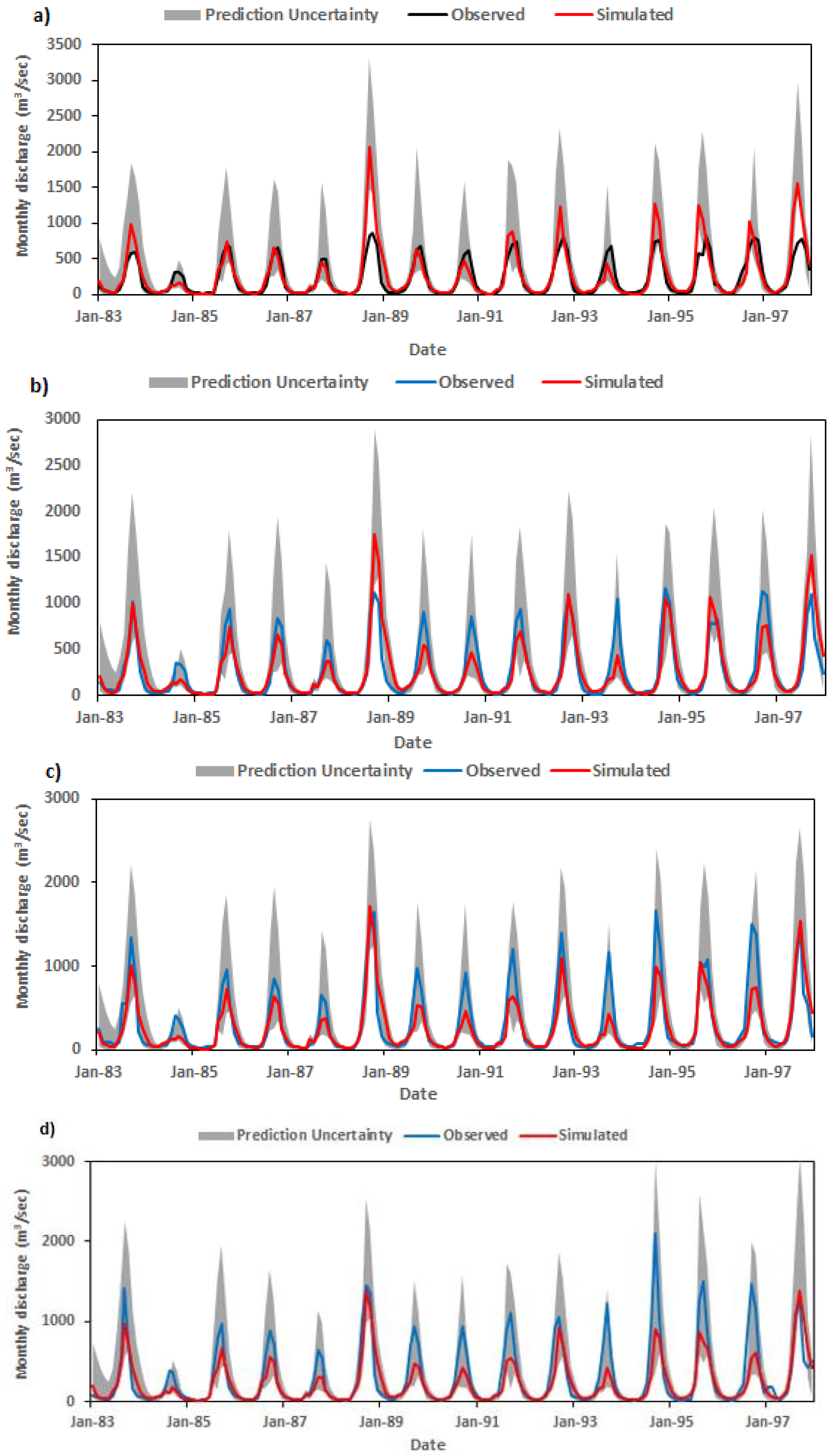
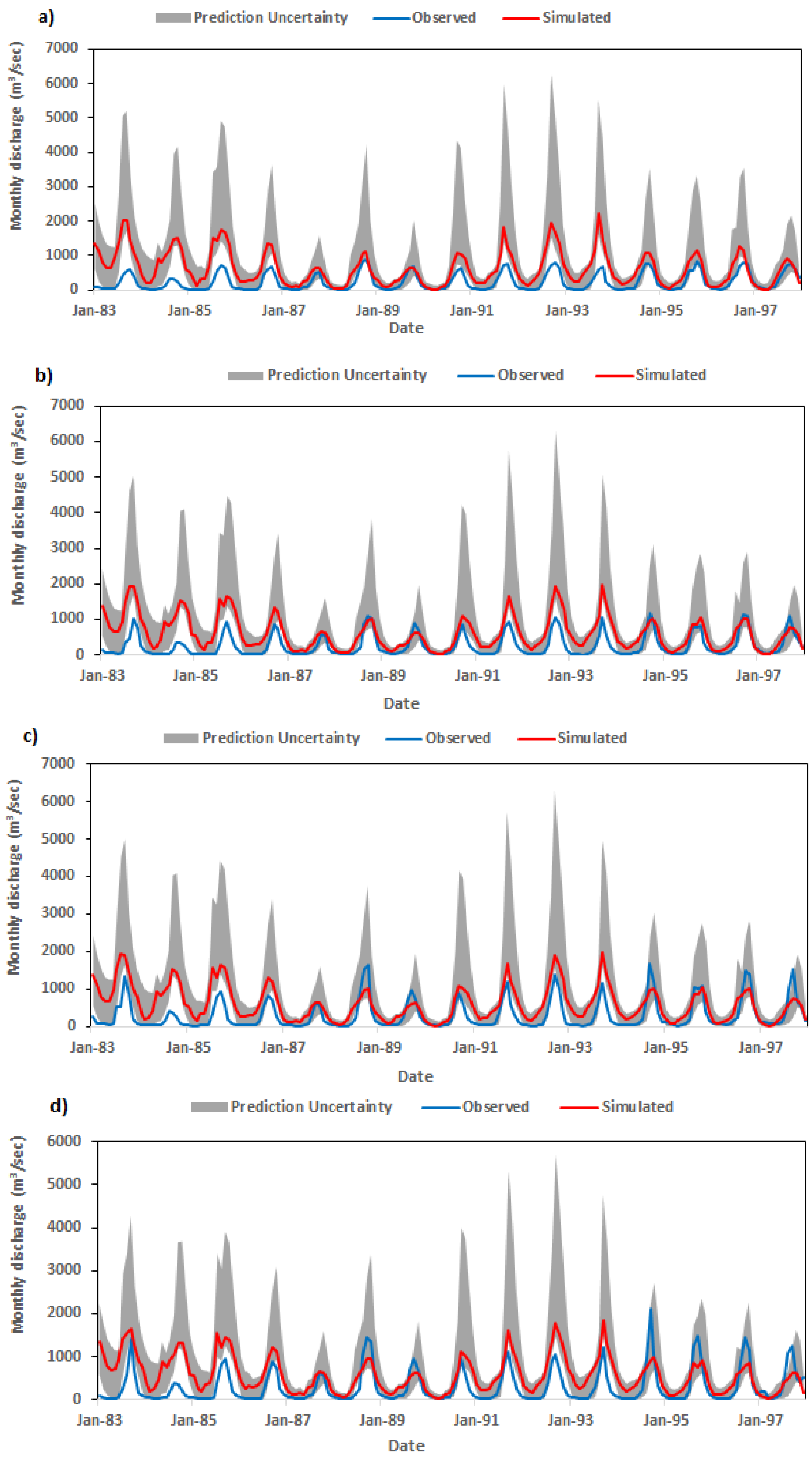
The model was calibrated in the SWAT Calibration and Uncertainty Program software (SWAT-CUP) using the Sequential Uncertainty Fitting algorithm (SUFI-2) [28]. During the calibration process in SUFI-2, parameters can be changed using either the relative or absolute parameter ranges. Each parameter value can be modified either by replacement of the initial value, addition of absolute change or multiplication by a relative change factor to obtain the optimum value. Given the multiple sources of uncertainties inherent in the use of hydrological models; the advantage of using SWAT-CUP is that these are taken into consideration during model calibration [28]. As model parameters often depend on the input data used to drive the model which is susceptible to seasonal variation [29]; the calibrated parameter values in SWAT-CUP are given within a range to represent this variability. Model calibration consisted of running 500 simulations in each iteration with the parameter set shown in

Table 1. Description of model parameters, parameter ranges used for calibration. The ranges are given for the three datasets used in the study.

Parameter	Description	Model Process	Parameter Range Used
CN2 a	Curve number for moisture condition II	Surface runoff generation. High values lead to high surface flow	−0.5–0.15
GW_Delay	Groundwater delay	Groundwater (affects groundwater movement). It is the lag between the time water exits the soil profile and enters the shallow aquifer	30–250
GW_REVAP	Groundwater “revap” coefficient	Affects the movement of water from the shallow aquifer to the unsaturated soil layers. Low values lead to high baseflow	0.10–0.40
GWQMN	Threshold depth of water in the shallow aquifer required for return flow to occur	Groundwater (when reduced streamflow increases)	20–95
Revapmn	Threshold depth of water for “revap to occur” (mm)	Groundwater (when increased, base flow will increase)	0–20
Rchrg_DP	Deep aquifer percolation	Groundwater (the fraction of percolation from the root zone which recharges the deep aquifer. Higher values lead to high percolation).	0.05–0.50
Ch_K2	Hydraulic conductivity of main channel	Channel infiltration	1.69–6.0
ESCO	Soil evaporation compensation factor	Controls the soil evaporative demand from different soil depth. High values lead to low evapotranspiration	0.25–0.95
SOL-AWC a	Available Water Capacity or available is calculated as the difference between field capacity the wilting point	Groundwater, evaporation. When increased less water is sent to the reach as more water is retained in the soil thus increasing evapotranspiration	−0.04–0.04
ALPHA_BF	Base flow alpha factor	Shows the direct index of groundwater flow response to changes in recharge	0.3–0.9
Surlag	Surface runoff lag coefficient	Surface runoff	1.5–5.0

^a Parameter value is multiplied by (1 + a given value). For example if CN2 = 85 then the calibrated CN2 value will be (1 +(−0.5)) × 85 = 0.5 × 85 = 42.5.

. The best parameter range obtained in the first iteration was then substituted and used in the next iteration for each of the five iterations performed. This was done for the three different datasets at daily and monthly time steps. To obtain the values of the different water balance components such as evapotranspiration, the simulation number that produced the best model output was used to calculate the water balance for the whole catchment.

The model was evaluated using three different evaluation statistics: (i) the Nash Sutcliffe Efficiency (NSE); (ii) coefficient of determination (R²); and (iii) Percent Bias (PBIAS). The NSE is used to assess the predictive capacity of the model and measures how well the observed and simulated flows match. Its value range from –∞ to 1 with values close to 1 indicating high model performance. The R² measures how well the observed data is correlated to the simulated data and varies from 0 to 1 with values closer to 1 also indicating high model performance. PBIAS indicates the average tendency of the simulated flows to be over/underestimated than observed flows with absolute low values indicating accurate model simulation. Positive values indicate model underestimation while negative values indicate overestimation. According to [30], the results of the calibrated model may be considered to be satisfactory if NSE > 0.50, R² > 0.60 and PBIAS ± 25%.

The degree of uncertainty in the calibrated model(s) was quantified using the p-factor and r-factor. The p-factor represents the percentage of observed streamflow bracketed by the 95% prediction uncertainty (95PPU) while the r-factor is the average width of the 95PPU. The 95PPU is calculated at the 2.5% and 97.5% confidence interval of observed streamflow obtained through Latin hypercube sampling. In SUFI-2, the goal is to minimize the width of the uncertainty band and enclose as many observations as possible because these observations are a result of all processes taking place in the catchment [28]. The p-factor can vary between 0 and 1 while the ideal value for r-factor is 0, indicating that there is no uncertainty in the model outputs. However, an r-factor of 0 will indicate that fewer flow observations were included in the 95PPU band.

Given that the goal of this study was to evaluate how well each reanalysis dataset was able to simulate streamflow as closely as possible to the observed, all parameters that influence this process, were calibrated. Evapotranspiration (ESCO); surface runoff (CN2, Surlag, Ch_K2); groundwater exchange (Rchrg_DP, GWQMN, GW_REVAP, REVAPMN, GW_DELAY, ALPHA_BF) and infiltration (SOL_AWC). Furthermore, since this study objective did not include evaluation of alternative scenarios for which it would be necessary to establish the performance limits of different parameter sets e.g., by validating the parameter set(s) using independent observations, the entire period of the available streamflow record was used for calibration. The advantage of this approach is that, longer input time series are included in the simulation with the possibility of capturing long term trends and variability as simulated by reanalysis forecast models. Auerbach et al. [31] used a similar approach to evaluate the performance of CFSR dataset as input for hydrological modelling in the tropics. Furthermore, the parameters range obtained during model over this long time scale could be used for climate change impact assessment in the catchment. The model was calibrated from 1980 to 1997 at daily and monthly time steps using the first three years as warm-up period. This calibration was done at Logone Gana, Katao, Bongor and Lai hydrometric stations (Figure 1).

3. Results

The optimum threshold area used for delineating the catchment into different sub catchments was 750 km². Using this area 57, 34 and 19 reanalysis grid points were selected for CFSR, WFDEI and ERA Interim respectively (Figure 1).

Figure 2 shows the variability in annual rainfall from the three datasets used in this study. It can be observed from the figure that the variability in the datasets is not the same because maximum and minimum rainfall occur in almost different years except in a few cases when all the datasets produced maximum/minimum rainfall in the same year e.g., 1985, 1988 and 1992. Annual rainfall from WFDEI varies between 1000 and 1300 mm/year, CFSR varies between 900–1550 mm/year and ERA-Interim varies between 750 and1650 mm/year. Overall the analysis showed that the variability is highest for ERA-Interim followed by CFSR while WFDEI has lowest variability in annual rainfall. The annual average rainfall in the catchment as simulated by SWAT model for the three datasets was 1237 mm, 1240 mm and 1047 mm for WFDEI, CFSR and ERA-Interim respectively indicating that ERA-Interim recorded the lowest amount of rainfall in the catchment for the period under study.

Results of model calibration are shown in

Table 2. Results of model calibration at daily and monthly time steps.

Time Step	Evaluation Criteria	WFDEI				CFSR				ERA Interim
		Gana	Katoa	Bongor	Lai	Gana	Katoa	Bongor	Lai	Gana	Katoa	Bongor	Lai
Daily	NSE	0.05	0.58	0.66	0.57	−0.67	0.17	0.43	0.31	−3.97	−1.54	−0.59	−0.56
	R2	0.64	0.68	0.68	0.6	0.65	0.62	0.57	0.51	0.47	0.44	0.38	0.31
	PBIAS (%)	−15.2	2.7	16.6	22.7	−74.5	−51.7	−32.3	−42.0	−146.1	−109.6	−81	−78.7
	p-factor	0.61	0.64	0.6	0.68	0.78	0.80	0.81	0.78	0.63	0.65	0.66	0.62
	r-factor	1.69	1.3	1.02	0.89	2.47	1.87	1.48	1.46	3.78	2.58	2.01	1.73
Monthly	NSE	0.43	0.75	0.77	0.67	−0.28	0.39	0.59	0.49	−3.12	−1.17	−0.38	−0.31
	R2	0.73	0.77	0.8	0.73	0.74	0.71	0.68	0.61	0.52	0.48	0.44	0.37
	PBIAS (%)	−16.2	3.5	17.7	23.6	−66.9	−45.4	−26.8	−36.6	−163.3	−125.5	−94.8	−91.4
	p-factor	0.86	0.88	0.81	0.83	0.68	0.73	0.78	0.74	0.64	0.66	0.67	0.63
	r-factor	1.65	1.26	1	0.87	2.04	1.55	1.25	1.23	3.41	2.6	2.09	1.86

for daily and monthly time steps respectively. It can be observed from the table that only WFDEI dataset produced NSE and R² values considered to be satisfactory according to Moriasi et al. [30] model evaluation criteria at both time steps for most hydrometric stations. CFSR and ERA-Interim both produced unsatisfactory results because most NSE values fall below the minimum threshold although the performance of the former was better compared to the latter. Generally, it was observed that there was a considerable improvement in NSE values at the monthly time step compared to daily for all datasets. For example, NSE values for WFDEI data improved from a range of 0.05–0.66 to 0.43–0.77 while that of CFSR improved from a range of −0.67–0.43 to −0.43–0.59. Despite a general under performance compared to WFDEI, CFSR registered negative NSE values at both time steps only at one hydrometric station (Logone Gana).

The PBIAS values obtained also showed that only WFDEI was able to produce values that fall within the acceptable limits while results from the other two datasets show a consistent over estimation of annual discharge throughout the simulation period at all hydrometric stations.

Results further show that all the datasets were able to replicate the streamflow seasonal cycle at all hydrometric stations. This follows the finding of Nkiaka et al. [21] who showed that CFSR and ERA-Interim precipitation estimates could replicate the seasonal cycle of rainfall in the catchment. However, from the streamflow hydrographs shown in Figure 3, Figure 4, Figure 5 and Figure 6 it can be observed that WFDEI and CFSR were able to simulate low flows (baseflow) throughout the period under study while ERA-Interim overestimated low flows in most years during the same period. Apart from a few cases of overestimation, the WFDEI dataset was able to simulate peak discharges at Logone Gana hydrometric station but consistently underestimated at other stations. Although there were a few cases of overestimation and a general underperformance compared to WFDEI; CFSR was able to simulate peak flows at most hydrometric stations compared to WFDEI and ERA-Interim (Figure 5). Only daily streamflow hydrographs for WFDEI are shown herein. Comparing the results of the other two reanalysis products showed that CFSR outperformed ERA-Interim. ERA-Interim consistently underestimated streamflow in 1987, 1989 and from 1994–1997 (Figure 6). This underestimation of discharge by ERA-Interim follows the general underestimation of average rainfall in the catchment during these years.

From Table 2 and Figure 3, Figure 4, Figure 5 and Figure 6, the p-factor values obtained indicate that more than 60% of observed streamflow values at all the hydrometric stations were bracketed within the 95PPU band at both time steps for all the datasets although CFSR outperformed WFDEI and ERA-Interim at daily time step. At the monthly time step, WFDEI outperformed the other two datasets with more than 80% of observed streamflow bracketed within the 95PPU band. Nevertheless, r-factor values obtained for CFSR and ERA-Interim as shown by Figure 5 and Figure 6 and Table 2 indicate that the uncertainty band for these datasets was much wider compared to that of WFDEI. This suggest that streamflow simulated using WFDEI dataset had the lowest level of uncertainty followed by CFSR while ERA-Interim produced the highest uncertainty.

Regarding the impact of spatial resolution of reanalysis datasets on streamflow simulation, results showed that WFDEI which has a lower spatial resolution (0.5°) compared to CFSR (0.312°) performed better than the latter in streamflow simulation given that the calibration results produced by the WFDEI are better than those of CFSR. Furthermore, the PBIAS values showed that CFSR with fine resolution compared to WFDEI consistently overestimated simulated streamflow during the period under study.

Analysis of water balance components showed that 74%, 65% and 58% of total rainfall received in the catchment was lost through evapotranspiration for WFDEI, CFSR and ERA-Interim respectively. Compared to the amount of rainfall received in the catchment, the evapotranspiration estimates from WFDEI compare well with the results of [32,33] obtained in the Ouemé river basin which is located in the same latitudinal zone with the Logone catchment.

4. Discussion

4.1. Selection of Grid Points

During the selection of grid points used as meteorological stations input in SWAT, the model selects each grid point depending on its proximity to the centroid of the sub catchment [27]. When low resolution reanalysis data is used to drive SWAT, the possibility of the model locating a grid point in each sub catchment may be reduced. This explains why many grid points (57) were selected for CFSR because of its high spatial resolution which is almost two times that of WFDEI with (34) grid points and three times that of ERA Interim (19) grid points. Even so, not every sub catchment had a different grid point because only 57 grid points were selected for CFSR instead of 66 to correspond to the number of sub-catchments in the catchment.

4.2. Model Evaluation

Results of model evaluation indices showed that WFDEI had the best performance among the three datasets. This is not surprising given that WFDEI had the best rainfall input among three datasets evaluated because of reduced variability in rainfall estimates. This demonstrates the importance of post-processing or bias correcting global reanalysis datasets before using them for hydrological modelling. The post-processing reduces the uncertainty in the rainfall data thus leading to better streamflow simulation. We therefore conclude that WFDEI outperformed the other two datasets (CFSR and ERA-Interim) in simulating streamflow in the Logone catchment due to reduced uncertainty in the rainfall estimates from this dataset as shown in Figure 2. These results are similar to those obtained by [18,19] who reported that WFDEI improved streamflow simulation compared to other global reanalysis datasets in their respective study areas. Meanwhile, [19] asserted that CFSR outperformed ERA-Interim in streamflow simulation in the Patagonia basin in South America.

Given that low flows and peak discharges were adequately simulated by WFDEI and CFSR datasets indicate that the parameter range(s) used to calibrate the model(s) can be considered to be satisfactory and cases of streamflow under/overestimation may be attributed to the uncertainty in the rainfall input used in calibrating the models or to parameter conditionality. This is because the same parameter set was used to calibrate the model in both semi-arid and Sudano areas; although the amount of rainfall received by each zone is different which has implications for parameter values used in calibrating the model.

The poor performance of ERA-Interim can be attributed to the high variability in annual rainfall produced by this dataset compared to the other two datasets. For example, Figure 2 shows that annual rainfall produced by ERA-Interim was consistently lower compared to the other two datasets in 1987, 1989 and 1994–1997 leading to a systematic underestimation of simulated streamflow by ERA-Interim during these years. This high variability in ERA-Interim rainfall estimates may have offset the interaction among the different model parameters making it difficult to find a parameter range that could simulate streamflow above the minimum threshold limit. This suggest that rainfall input plays a significant role in model calibration because it has the potential to influence calibrated parameters as reported by [29]. Nevertheless, the significant variability in CFSR and ERA-Interim datasets in this study follow the findings of [21] in the Logone catchment.

4.3. Prediction Uncertainty

The daily streamflow hydrographs with corresponding prediction uncertainty band and rainfall input shown in Figure 3 indicate that, as the variability in rainfall input increases, the values of r-factor, which measures the prediction uncertainty band increases as well. This indicates that rainfall input contributes significantly to increase the level of uncertainty in the simulated streamflow because as the variability in rainfall increases, the uncertainty band also increases. This suggests that, reducing the variability in the rainfall input or accurately estimating the rainfall data used for driving the model could lead to a significant improvement in simulated streamflow thereby reducing the level of uncertainty in the latter. This follows the findings of [13] who asserted that performance of reanalysis datasets in hydrological modelling depends largely on the quality of the rainfall data.

The improved performance of model evaluation indices and improvement in model uncertainty at monthly time steps compared to daily can be attributed to the fact that, monthly rainfall is a cumulative measurement in which all the daily variability within the month is summed, thus reducing the variability in the input data which leads to an overall improvement in model performance.

Nevertheless, it is worth noting that the contribution of model parameters to the overall uncertainty in the simulated streamflow cannot be overlooked since it is difficult to decouple the uncertainty inherent in model parameters from that of input data [9]. It should be noted that assessing the uncertainty of model parameters was not part of this study.

The high variability in rainfall estimates from the reanalysis datasets in the study area can be attributed to the low rain gauge density and few radiosonde coverages in Central Africa [11,34] used for optimization and data-assimilation in the reanalysis forecast models thus increasing the forcing uncertainty. According to Sperna Weiland [35], when using global reanalysis datasets for hydrological modelling, the forcing uncertainty decreases with increasing number of sampling points available for optimization and data-assimilation, suggesting that a limited number of sampling points will lead to an increased level of forcing uncertainty. Although WFDEI has fewer grid points compared to CFSR, the improvement of WFDEI rainfall estimates compared to CFSR can be attributed to the fact that this dataset is bias corrected.

4.4. Effects of Spatial Resolution

The results obtained from this study also suggest that streamflow simulation may not represent an important factor to be used for evaluating the impact of spatial resolution of reanalysis datasets as long as the average rainfall over the modelled catchment is accurately estimated. This is because in moderate size catchments such as the Logone, the model integrates rainfall data from a very large area which dampens and smooths the impact of rainfall spatial variability on the catchment outflow, hence limiting the effect of spatial resolution on streamflow. Under such circumstances, the ability of the reanalysis product to produce accurate precipitation estimates in the catchment is more important than its spatial resolution. Gascon et al. [36] also demonstrated that the spatial resolution of rainfall datasets had no significant impact on streamflow simulation in the Ouémé basin. These authors used rainfall datasets at spatial resolutions of 0.05°, 0.1°, 0.25° and 0.5°. Results from this study also corroborate the findings of Fu et al. [37], where the authors demonstrated that, the impact of rainfall spatial resolution was insignificant for catchment sizes above 250 km² and negligible for catchments larger than 1000 km². A recent study, [15] demonstrated that, the impact of spatial resolution on flow simulation was scale, catchment and event characteristic-dependent. We conclude that, the ability of the reanalysis dataset(s) to accurately produce good quality rainfall estimates in the study area can significantly improve streamflow simulation compared to the spatial resolution of the rainfall. Nevertheless, Tramblay et al. [38] have shown that spatial rainfall representation is important in the simulation of flood events.

4.5. Simulation of Evapotranspiration

The values of actual evapotranspiration estimates obtained showed that there were significant differences in the values produced by the threedatasets. These differences in actual evapotranspiration values from the different datasets can be attributed to the different amounts of rainfall input used in simulating each model. WFDEI and CFSR produced almost the same amount of average rainfall during the simulation period but there is a significant discrepancy between the actual evapotranspiration values from the two datasets. This discrepancy can be attributed to the uncertainty inherent in each of the r datasets. This is because precipitation estimates can strongly influence the parameter values that control the rates and threshold of hydrological processes taking place in the catchment [39]. Furthermore, as pointed out by Remesan and Holman [39] our results show that the uncertainty in the rainfall estimates is conserved and propagated into streamflow and other water balance components including evapotranspiration. Although ground data was not available to compare the evapotranspiration estimates in this study, the estimates from WFDEI are acceptable given that similar values have been obtained in other catchments the region [32,33]. Furthermore, the importance of temperature in influencing actual evapotranspiration cannot be overstated implying that the minimum and maximum temperature estimates used in the simulations could also interact to strongly influence the results obtained.

We conclude that the estimation of actual evapotranspiration and other water balance components by the model is influenced by the precipitation estimates and other input data used in driving the model.

5. Conclusions

The objectives of this study were to evaluate the ability of two global reanalysis datasets; CFSR and ERA-Interim and one bias corrected global meteorological forcing dataset WFDEI to be used as input to drive the SWAT model in the Logone catchment, and to evaluate the impact of reanalysis spatial resolution on the quality of simulated flows.

The results of our study showed that the WFDEI out-performed the other two datasets in simulating streamflow in the study area. This highlights the importance of bias correcting global reanalysis datasets before using them for hydrological modelling. As seen in the hydrographs of WFDEI, the bias correction reduces the uncertainty in precipitation estimates used to drive the hydrological model which has a direct positive impact in reducing the overall uncertainty in the simulated streamflow.

The results obtained also showed that the ability of reanalysis forecast models to produce accurate precipitation estimates is more important than its spatial resolution. This is because accurate streamflow simulation and hydrological modelling in general depend on accurate rainfall input given that the impacts of spatial resolution on streamflow simulation are not significant in medium to large catchments.

From the result of evapotranspiration estimates obtained, we conclude that the estimation of actual evapotranspiration depends on the input data used in driving the model. This is because rainfall, temperature and other variables play a significant role in influencing model parameters that interact to control hydrological processes, e.g., evapotranspiration at catchment scales.

Finally, we conclude that in the absence of gauged hydro-meteorological data, WFDEI and CFSR could be used for hydrological modelling in data-scarce areas such as the Sudano-Sahel and other remote locations with poor data availability.

This study is part of an on-going research aimed at understanding the hydrological dynamics of the Logone catchment with the aim of improving water resources management. Future research in the catchment will use the WFDEI dataset, which has been shown to out-perform the other two datasets in this study, for detailed hydrological analysis of the catchment to determine the main processes and feedback mechanisms driving the response of the catchment to natural and anthropogenic changes.

References

1. Van de Giesen, N.; Hut, R.; Selker, J. The trans-African hydro-meteorological observatory (TAHMO). WIREs Water. 2014, 1, 341–348. [Google Scholar] [CrossRef]
2. Buma, W.G.; Lee, S.; Seo, J.Y. Hydrological evaluation of Lake Chad basin using space borne and hydrological model observations. Water 2016, 8, 205. [Google Scholar] [CrossRef]
3. Buytaert, W.; Friesen, J.; Liebe, J.; Ludwig, R. Assessment and management of water resources in developing, semi-arid and arid regions. Water Resour. Manag. 2012, 26, 841–844. [Google Scholar] [CrossRef]
4. Gorgoglione, A.; Gioia, A.; Iacobellis, V.; Piccinni, A.F.; Ranieri, E. A rationale for pollutograph evaluation in ungauged areas, using daily rainfall patterns: Case studies of the Apulian region in Southern Italy. Appl. Environ. Soil Sci. 2016, 2016, 9327614. [Google Scholar] [CrossRef]
5. Liu, Y.; Gupta, H.; Springer, E.; Wagener, T. Linking science with environmental decision making: Experiences from an integrated modeling approach to supporting sustainable water resources management. Environ. Model. Softw. 2008, 23, 846–858. [Google Scholar] [CrossRef]
6. Worqlul, A.W.; Maathuis, B.; Adem, A.A.; Demissie, S.S.; Langan, S.; Steenhuis, T.S. Comparison of rainfall estimations by TRMM 3B42, MPEG and CFSR with ground-observed data for the Lake Tana basin in Ethiopia. Hydrol. Earth Syst. Sci. 2014, 18, 4871–4881. [Google Scholar] [CrossRef]
7. Fuka, D.R.; MacAllister, C.A.; Degaetano, A.T.; Easton, Z.M. Using the Climate Forecast System Reanalysis dataset to improve weather input data for watershed models. Hydrol. Process. 2013, 28, 5613–5623. [Google Scholar] [CrossRef]
8. Skinner, C.J.; Bellerby, T.J.; Greatrex, H.; Grimes, D.I.F. Hydrological modelling using ensemble satellite rainfall estimates in a sparsely gauged river basin: The need for whole ensemble calibration. J. Hydrol. 2015, 522, 110–122. [Google Scholar] [CrossRef]
9. Saha, S.; Moorthi, S.; Wu, X.; Wang, J.; Nadiga, S.; Tripp, P.; Behringer, D.; Hou, Y.-T.; Chuang, H.-Y.; Iredell, M. The NCEP climate forecast system version 2. J. Clim. 2014, 27, 2185–2208. [Google Scholar] [CrossRef]
10. Dee, D.P.; Uppala, S.M.; Simmons, A.J.; Berrisford, P.; Poli, P.; Kobayashi, S.; Andrae, U.; Balmaseda, M.A.; Balsamo, G.; Bauer, P.; et al. The ERA-Interim reanalysis: Configuration and performance of the data assimilation system. Q. J. R. Meteorol. Soc. 2011, 137, 553–597. [Google Scholar] [CrossRef]
11. Rienecker, M.M.; Suarez, M.J.; Gelaro, R.; Todling, R.; Bacmeister, J.; Liu, E.; Bosilovich, M.G.; Schubert, S.D.; Takacs, L.; Kim, G.-K.; et al. MERRA: NASA’s modern-era retrospective analysis for research and applications. J. Clim. 2011, 24, 3624–3648. [Google Scholar] [CrossRef]
12. Lorenz, C.; Kunstmann, H. The hydrological cycle in three state-of-the-art reanalyses: Intercomparison and performance analysis. J. Hydrometeorol. 2012, 13, 1397–1420. [Google Scholar] [CrossRef]
13. Essou, G.R.C.; Sabarly, F.; Lucas-Picher, P.; Brissette, F.; Poulin, A. Can precipitation and temperature from meteorological reanalyses be used for hydrological modelling? J. Hydrometeorol. 2016, 17, 1929–1950. [Google Scholar] [CrossRef]
14. Weedon, G.P.; Balsamo, G.; Bellouin, N.; Gomes, S.; Best, M.J.; Viterbo, P. The WFDEI meteorological forcing data set: WATCH forcing data methodology applied to ERA-Interim reanalysis data. Water Resour. Res. 2014, 50, 7505–7514. [Google Scholar] [CrossRef]
15. Zhao, F.; Zhang, L.; Chiew, F.H.S.; Vaze, J.; Cheng, L. The effect of spatial rainfall variability on water balance modelling for south-eastern Australian catchments. J. Hydrol. 2013, 493, 16–29. [Google Scholar] [CrossRef]
16. Lobligeois, F.; Andréassian, V.; Perrin, C.; Tabary, P.; Loumagne, C. When does higher spatial resolution rainfall information improve streamflow simulation? An evaluation using 3620 flood events. Hydrol. Earth Syst. Sci. 2014, 18, 575–594. [Google Scholar] [CrossRef] [Green Version]
17. Monteiro, J.A.F.; Strauch, M.; Srinivasan, R.; Abbaspour, K.; Gücker, B. Accuracy of grid precipitation data for Brazil: Application in river discharge modelling of the Tocantins catchment. Hydrol. Process. 2016, 30. [Google Scholar] [CrossRef]
18. Andersson, J.C.M.; Pechlivanidis, I.G.; Gustafsson, D.; Donnelly, C.; Arheimer, B. Key factors for improving large-scale hydrological model performance. Eur. Water. 2015, 49, 77–88. [Google Scholar]
19. Krogh, S.A.; Pomeroy, J.W.; McPhee, J. Physically based mountain hydrological modelling using reanalysis data in Patagonia. J. Hydrometeorol. 2015, 16, 172–193. [Google Scholar] [CrossRef]
20. Nkiaka, E.; Rizwan, N.R.; Lovett, J.C. Analysis of rainfall variability in the Logone catchment, Lake Chad basin. Int. J. Climatol. 2016. [Google Scholar] [CrossRef]
21. Nkiaka, E.; Rizwan, N.R.; Lovett, J.C. Evaluating global reanalysis precipitation datasets with rain gauge measurements in the Sudano-Sahel region: Case study of the Logone catchment, Lake Chad Basin. Meteorol. Appl. 2016, 24, 9–18. [Google Scholar] [CrossRef]
22. Siam, M.S.; Demory, M.; Eltahir, E.A.B. Hydrological cycles over the Congo and upper Blue Nile basins: Evaluation of general circulation model simulations and reanalysis products. J. Clim. 2013, 26, 8881–8894. [Google Scholar] [CrossRef]
23. Loth, P. The Return of the Water: Restoring the Waza Logone Floodplain in Cameroon; IUCN: Cambridge, UK, 2004. [Google Scholar]
24. Nkiaka, E.; Rizwan, N.R.; Lovett, J.C. Using self-organizing maps to infill missing data in hydro-meteorological time series from the logone catchment, Lake Chad basin. Environ. Monit. Assess. 2016, 188, 400. [Google Scholar] [CrossRef] [PubMed]
25. Morse, A.; Caminade, C.; Tompkins, A.; McIntyre, K.M. The QWeCI Project (Quantifying Weather and Climate Impacts on Health in Developing Countries); Final Report; Liverpool: University of Liverpool, UK, 2013. [Google Scholar]
26. Gassman, P.W.; Sadegh, I.A.M.; Srinivasan, R. Applications of the SWAT model special section: Overview and insights. J. Environ. Qual. 2014, 43, 1–8. [Google Scholar] [CrossRef] [PubMed]
27. Neitsch, S.L.; Arnold, J.G.; Kiniry, J.R.; Williams, J.R. Soil and Water Assessment Tool Theoretical Documentation Version 2009; Technical Report 406; Texas Water Resources Institute: Temple, TX, USA, 2011. [Google Scholar]
28. Abbaspour, K.C. SWAT-CUP: SWAT Calibration and Uncertainty Programs: A User Manual; Swiss Federal Institute of Aquatic Science and Technology: Eawag, Switzerland, 2015. [Google Scholar]
29. Pathiraja, S.; Marshall, L.; Sharma, A.; Moradkhani, H. Hydrologic modeling in dynamic catchments: A data assimilation approach. Water Resour. Res. 2016, 52, 3350–3372. [Google Scholar] [CrossRef]
30. Moriasi, D.N.; Arnold, J.G.; van Liew, M.W.; Bingner, R.L.; Harmel, R.D.; Veith, T.L. Model evaluation guidelines for systematic quantification of accuracy in watershed simulations. Trans. Asabe 2007, 50, 885–900. [Google Scholar] [CrossRef]
31. Auerbach, D.A.; Easton, Z.M.; Walter, M.T.; Flecker, A.S.; Fuka, D.R. Evaluating weather observations and the climate forecast system reanalysis as inputs for hydrologic modelling in the tropics. Hydrol. Process. 2016, 30, 3466–3477. [Google Scholar] [CrossRef]
32. Sintondji, L.O.; Zokpodo, B.; Ahouansou, D.M.; Vissin, W.E.; Agbossou, K.E. Modelling the water balance of Ouémé catchment at the Savè outlet in Benin: Contribution to the sustainable water resource management. Int. J. Agric. Sci. 2014, 4, 74–88. [Google Scholar]
33. Giertz, S.; Diekkrugerm, B.; Jaeger, A.; Schopp, M. An interdisciplinary scenario analysis to assess the water availability and water consumption in the upper Oueme catchment in Benin. Adv. Geosci. 2006, 9, 3–13. [Google Scholar] [CrossRef]
34. Maidment, R.I.; Grimes, D.I.F.; Allan, R.P.; Greatrex, H.; Rojas, O.; Leo, O. Evaluation of satellite-based and model re-analysis rainfall estimates for Uganda. Meteorol. Appl. 2013, 20, 308–317. [Google Scholar] [CrossRef]
35. Sperna Weiland, F.C.; Vrugt, J.A.; van Beek, R.P.H.; Weerts, A.H.; Bierkens, M.F.P. Significant uncertainty in global scale hydrological modeling from precipitation data errors. J. Hydrol. 2015, 529, 1095–1115. [Google Scholar] [CrossRef]
36. Gascon, T.; Vischel, T.; Lebel, T.; Quantin, G.; Pellarin, T.; Quatela, V.; Leroux, D.; Galle, S. Influence of rainfall space-time variability over the Ouémé basin in Benin. Proc. Int. Assoc. Hydrol. Sci. 2015, 368, 102–107. [Google Scholar] [CrossRef]
37. Fu, S.; Sonnenborg, T.O.; Jensen, K.H.; He, X. Impact of precipitation spatial resolution on the hydrological response of an integrated distributed water resources model. Vadose Zone J. 2011, 10, 25–36. [Google Scholar] [CrossRef]
38. Tramblay, Y.; Bouvier, C.; Ayral, P.-A.; Marchandise, A. Impact of rainfall spatial distribution on rainfall-runoff modelling efficiency and initial soil moisture conditions estimation. Nat. Hazards Earth Syst. Sci. 2011, 11, 157–170. [Google Scholar] [CrossRef]
39. Remesan, R.; Holman, I.P. Effect of baseline meteorological data selection on hydrological modelling of climate change scenarios. J. Hydrol. 2015, 528, 631–642. [Google Scholar] [CrossRef] [Green Version]
Figure 1. Map of the study area showing the Logone river network, sub catchments and reanalysis grid points used for streamflow simulation. DEM: Digital Elevation Model in metres.
Hydrology 04 00013 g001
Figure 2. Reanalysis annual rainfall variability in the Logone catchment.
Hydrology 04 00013 g002
Figure 3. WATCH Forcing Data methodology applied to ERA-Interim (WFDEI) daily hydrographs for observed and simulated flows at (a) Logone Gana; (b) Katoa and (c) Bongor (d) Lai.
Hydrology 04 00013 g003
Figure 4. WFDEI monthly hydrographs for observed and simulated flows at (a) Logone Gana; (b) Katoa and (c) Bongor (d) Lai.
Hydrology 04 00013 g004
Figure 5. Climate Forecasting System Reanalysis (CFSR) monthly hydrographs for observed and simulated flows at (a) Logone Gana; (b) Katoa and (c) Bongor (d) Lai.
Hydrology 04 00013 g005
Figure 6. European Center for Medium-Range Weather Forecasts (ECMWF) ERA-Interim monthly hydrographs for observed and simulated flows at (a) Logone Gana; (b) Katoa and (c) Bongor (d) Lai.
Hydrology 04 00013 g006