Exact and Approximate Solutions of Fractional Partial Differential Equations for Water Movement in Soils

Abstract

This paper presents solutions of the fractional partial differential equation (fPDE) for analysing water movement in soils. The fPDE explains processes equivalent to the concept of symmetrical fractional derivatives (SFDs) which have two components: the forward fractional derivative (FFD) and backward fractional derivative (BFD) of water movement in soils with the BFD representing the micro-scale backwater effect in porous media. The distributed-order time-space fPDE represents water movement in both swelling and non-swelling soils with mobile and immobile zones with the backwater effect operating at two time scales in large and small pores. The concept of flux-concentration relation is now updated to account for the relative fractional flux of water movement in soils.

1. Introduction

Water movement on the surface of the soil, into and out of the subsurface terrain, is a process which interfaces the atmosphere and the subsurface through physical infiltration and evaporation as well as transpiration by plants. Understanding of the movements of water into and out of the soils in different saturated states and through aquifers requires knowledge which connects soil science, groundwater hydrology, fluid mechanics and other related topics.

In this paper the water movement in soils of finite depths is investigated by presenting analytical solutions of the fractional partial differential equation (fPDE) of water movement. The fPDE discussed in this paper is one special form of the fPDEs presented earlier [1] following the extensive analysis and parameterisation of the flow processes in soils. The fPDEs incorporate both the material coordinate for water movement in swelling-shrinking soils and the Cartesian coordinates in non-swelling soils. For the derivation of the fPDE for water flow in soils, the connection has been established between the mass-time and space-time fPDEs and the continuous-time random walk (CTRW) theory. We also clarify that the fPDEs presented earlier based on the CTRW concept [2,3] incorporate the forward fractional derivative (FFD) and backward fractional derivative (BFD) introduced by Bochner [4] and demonstrated by Saichev and Zaslavsky [5] and Zaslavsky [6].

This paper further investigates water movement in non-swelling soils by presenting solutions with known boundary conditions for a finite soil profile. The solutions are also applicable to a material coordinate for swelling soils where the finite mass is used instead of the finite depth. These analyses are based on models formulated for water flow in soils with or without an immobile zone, and consider the following major issues in soil water movement:

(1) Swelling and non-swelling properties of soils;

(2) Mobile and immobile zones in soils are optional. The mobile-immobile concept, which was first proposed by Barenblatt et al. in 1960 [7], is taken into account in both the mass-time and space-time fPDEs;

(3) The connection between the mass-time fPDEs and CTRW theory for soils is further discussed, and

(4) Space-time scaling laws [6] are briefly discussed for the fPDEs in the context of mass-time and space-time fractional derivatives.

The CTRW is a further development from the concept of the random walk which was first mathematically illustrated by Crofton [8] in terms of random flights as an alternative term, and later used by Pearson [9]. This concept was successfully employed to model solute movement in porous media by Saffman [10]. The CTRW theory for particle transport is understood in the framework of the classical renewal theory [11]. The mechanics of flow in porous media can be ideally described by the CTRW theory, and the phenomena described by the CTRW concept is anomalous which is a generalisation of the transport processes with the classic diffusion as a special case [3].

The mass-time fPDE is an extension of the space-time fPDE, which is a consequence of the long-time limit or asymptotic result of the two probability density functions of the CTRW model with power-law waiting times and power-law jumps [2,3,6,12]. These distributed-order fPDEs with convection included form the mass-time fractional advection-diffusion equation (fADE) and the space-time fADE. This connection offers another option for deriving the fPDE-based models without resorting to the traditional mass balance method for their derivation.

The symmetrical fractional derivatives (SFDs) include both the backward fractional derivative (BFD) and the forward fractional derivatives (FFD) in space. The BFD is capable of accounting for the backwater effect on particle and water parcel motion at a micro-scale, compared to the well-known large-scale backwater effect in hydraulics.

The multi-term fractional derivatives in time used in the fPDE by Hadid and Luchko [13] and Jiang et al. [14] are an ideal way to model flow and particle motion in fractal media with an unlimited level of micro-structures, which is a key characteristic of fractal media. In this paper a two-term Mittag-Leffler function is used in the solution to account for the mobile-immobile zone as an approximation to the multinomial Mittag-Leffler function. The examples of mobile-immobile models include those for solute transport in saturated media by Schumer et al. [15], water flow in unsaturated soils by Su [1,16] and saturated aquifers [17].

By combining the BFD and the widely-used two-term mobile-immobile model, the fPDE is expected to embrace more processes and provide informative insights into processes of water flow in soils.

2. The CTRW Theory and Its Connection with the fPDE for Water Movement in Soils with Wandering Processes

In a comprehensive development [1], we have introduced a set of fPDEs for water flow in both swelling and non-swelling soils. For swelling soils, with the material diffusivity given by

$$D_m(\mathsf{\theta })=D_0{\mathsf{\theta }}^b$$

(1)

and the hydraulic conductivity by

$$K_m(\mathsf{\theta })=\left({\gamma }_n\alpha -1\right)K_0{\mathsf{\theta }}^k$$

(2)

where $D_0$, $b$, $K_0$ and $k$ are constants, the equation governing the movement of water in swelling soils is given as

$$\begin{array}{cc}{b}_1\frac{{\partial }^{{\beta }_1}\mathsf{\theta }}{\partial t^{{\beta }_1}}+b_2\frac{{\partial }^{{\beta }_2}\mathsf{\theta }}{\partial t^{{\beta }_2}}\hfill & =\frac{{\partial }^{\mu }q}{\partial m^{\mu }}-\frac{\partial K_m}{\partial m}\hfill \\ & =\frac{D_0}{b+1}\frac{{\partial }^{\lambda }{\mathsf{\theta }}^{b+1}}{\partial m^{\lambda }}-\left({\gamma }_n\alpha -1\right)K_0\frac{\partial {\mathsf{\theta }}^k}{\partial m}\hfill \end{array}$$

(3)

where $q$ is the Darcy’s flux, $\lambda =\mu +1$ and $m$ is the material coordinate defined by [18,19]

$$m={\displaystyle \underset{0}{\overset{z}{\int }}{\left(1+e\right)}^{-1}d{z}_1}$$

(4)

where $m$ is the conventional space coordinate in a vertical direction, and $e$ is the void ratio given by $e=\mathsf{\theta }/(1-\mathsf{\theta })$ with $\mathsf{\theta }$ the moisture ratio defined as $\mathsf{\theta }={\mathsf{\theta }}_l/{\mathsf{\theta }}_s$, and ${\mathsf{\theta }}_{\mathrm{l}}$ and ${\mathsf{\theta }}_s$ being the volume fractions of liquid and solid, respectively;

$b_1$ and $b_2$ are the relative porosities in immobile and mobile zones, respectively, i.e., $b_1=\frac{{\mathsf{\phi }}_{im}}{\mathsf{\phi }}$ and $b_2=\frac{{\mathsf{\phi }}_m}{\mathsf{\phi }}$ with ${\mathsf{\phi }}_{im}$, ${\mathsf{\phi }}_m$ and $\mathsf{\phi }$ being the porosities in the immobile and mobile zones, and total porosity, respectively;

${\beta }_1$ and ${\beta }_2$ are the orders of fractional derivatives for immobile and mobile zones, respectively;

${\gamma }_n$ is the particle specific gravity, and

$\alpha$ is the gradient (or slope) of the shrinkage curve, which is a ratio on the graph of the specific volume, $v$, versus water content or moisture ratio, $\mathsf{\theta }$.

The equation for water movement in one dimension in non-swelling soils is of the form

$$b_1\frac{{\partial }^{{\beta }_1}\mathsf{\theta }}{\partial t^{{\beta }_1}}+b_2\frac{{\partial }^{{\beta }_2}\mathsf{\theta }}{\partial t^{{\beta }_2}}=\frac{D_0}{b+1}\frac{{\partial }^{\lambda }{\mathsf{\theta }}^{b+1}}{\partial z^{\lambda }}-K_0\frac{\partial {\mathsf{\theta }}^k}{\partial z}$$

(5)

where the power functions similar to Equations (1) and (2) are used for the diffusivity and hydraulic conductivity for non-swelling soils, respectively. Multidimensional fPDEs have also been presented for water flow in non-swelling soils [1].

Equations (3) and (5) were derived based on the CTRW theory, and the notations used for their derivation are identical to those in Gorenflo and Mainardi [2,20] and Gorenflo et al. [3]. Here we should emphasise that the SFDs in [2,3,20] are identical terminologies in Saichev and Zaslavsky [5] who derived fPDEs by defining the concept of “wandering process” with the BFD and FFD illustrated by Bochner [4]. See Appendix A in this paper for more details.

For water movement in two directions in swelling soils, the BFD and FFD are denoted using the sign $\left|m\right|$ and Equation (3) can be more generally written as

$$b_1\frac{{\partial }^{{\beta }_1}\mathsf{\theta }}{\partial t^{{\beta }_1}}+b_2\frac{{\partial }^{{\beta }_2}\mathsf{\theta }}{\partial t^{{\beta }_2}}=\frac{D_0}{b+1}\frac{{\partial }^{\lambda }{\mathsf{\theta }}^{b+1}}{\partial {\left|m\right|}^{\lambda }}-\left({\gamma }_n\alpha -1\right)K_0\frac{{\partial }^{\eta }{\mathsf{\theta }}^k}{\partial {\left|m\right|}^{\eta }}$$

(6)

$$\begin{array}{cc}0<{\mathsf{\beta }}_1\le 2;\hfill & \hfill 0<{\mathsf{\beta }}_2\le 2\\ 0<\mathsf{\lambda }\le 2;\hfill & \hfill b_1+b_2=1\end{array}\}$$

(7)

which is the mass-time distributed-order fADE for water movement in swelling soils with the material coordinate being dependent on the moisture ratio. In other words, the term $\frac{{\partial }^{\mathsf{\lambda }}\mathsf{\theta }}{\partial {\left|m\right|}^{\mathsf{\lambda }}}$ in Equation (6) includes both the forward and backward fractional components if the particle or water parcel motion is regarded as a wandering process [5].

Equation (6) is based on the CTRW theory with distributed-order time fractional derivatives resulting from the two time-scaling property and convection due to a shift jump size distribution in the CTRW theory [21]. The connection between CTRW and the distributed-order fPDE has been established [22], which is also applicable to Equation (6) and is an extension of the CTRW theory and fPDE to swelling soils.

The parameters and the material coordinate in Equation (6) characterise the different flow patterns in swelling soils with mobile and immobile zones which have a variable material diffusivity, $D_m(\theta )$ and hydraulic conductivity, $K_m(\theta )$ as functions of the moisture ratio.

Similar to Equation (6) for swelling soils, Equation (5) for non-swelling soils can be more generally written as

$$b_1\frac{{\partial }^{{\beta }_1}\theta }{\partial t^{{\beta }_1}}+b_2\frac{{\partial }^{{\beta }_2}\theta }{\partial t^{{\beta }_2}}=\frac{D_0}{b+1}\frac{{\partial }^{\lambda }{\theta }^{b+1}}{\partial {\left|z\right|}^{\lambda }}-K_0\frac{{\partial }^{\eta }{\theta }^k}{\partial {\left|z\right|}^{\eta }}$$

(8)

$$\begin{array}{cc}0<{\mathsf{\beta }}_1\le 2;\hfill & \hfill 0<{\mathsf{\beta }}_2\le 2\\ 0<\mathsf{\lambda }\le 2;\hfill & \hfill b_1+b_2=1\end{array}\}$$

(9)

where $z$ is the usual physical coordinate.

The large-scale backwater effect is well known in hydraulics. With the BFD concept in space, the backwater effect is now extended to flow at a micro-scale, and the distributed-order time fPDE for water movement with the forward and backward fractional derivatives accounts for the anomalous water movement with the backwater effect at two time-scales in soils.

Similar to Equations (8) and (A6) and (A7) in the Appendix, the signs of $\frac{{\partial }^{\lambda }\theta }{\partial {\left|z\right|}^{\lambda }}$ and $D_0^{\lambda }\theta$ for non-swelling soils are identical, then $\frac{{\partial }^{\lambda }\theta }{\partial {\left|z\right|}^{\lambda }}=D_0^{\lambda }\theta$ is used throughout the text as the synonyms of the SFDs.

Compared to the classic advection-diffusion equation (ADE), the space- and time-fractional models are shown to better represent the first and second moments of solute transport at early times and the tails of tracer plumes [21]. As water is the carrier of the solutes in soils, the fractional model is then expected to perform better than its classic counterpart for water flow in soils, particularly at the early and final stages of infiltration processes at the soil surface.

3. Solutions of the Distributed-Order Fractional Partial Differential Equations Incorporating Forward and Backward Motion of Water Flow in Soils

Here we present solutions of Equation (8), the space-time fPDE for water flow in non-swelling soils, which are also applicable to Equation (6) with the only difference being $m$ replacing $z$. The solutions presented here are modifications of those given by Jiang et al. [14] with only two terms of time fractional derivatives retained to account for the two-zone model (the mobile-immobile or large-small porosity model) for flow in porous media. The solutions are subject to the following initial condition (IC) and boundary conditions (BCs),

$$\theta (z,t)=\theta (z,0), t=0, 0<z<L$$

(10)

$$\theta (z,t)=\theta (0,t), t\ge 0, z=0$$

(11)

$$\theta (z,t)=\theta (L,t), t\ge 0, z=L$$

(12)

where $L$ is the depth of the soil profile.

The moisture ratios on the surface and the depth $z=L$ are, respectively, $\mathsf{\theta }(0,t)$ and $\mathsf{\theta }(L,t)$. The complete solution of Equation (8) subject to the above conditions is Equation (B12) in Appendix B, and the approximate solution by retaining the first term of the full solution is as follows,

$$\theta (z,t)=\theta (0,t)+a_{2}z+\frac{1}{\pi }\left\{\frac{2a_{2}L}{\pi }{\sin }^2\left(\frac{\pi z}{L}\right)-\left(a_1+a_{2}z\right)\sin \left(\frac{2\pi z}{L}\right)\right\}F(t)$$

(13)

where

$$F(t)=1-K_1{t}^{{\mathsf{\beta }}_2}\left(\frac{1}{{\Gamma }_{[1+{\mathsf{\beta }}_2]}}+\frac{b_1{t}^{-{\mathsf{\beta }}_1}}{K_1{b}_2{\Gamma }_{[1+{\mathsf{\beta }}_2-{\mathsf{\beta }}_1]}}-\frac{K_1{t}^{{\mathsf{\beta }}_2}}{{\Gamma }_{[1+2{\mathsf{\beta }}_2]}}-\frac{b_1{t}^{{\mathsf{\beta }}_2-{\mathsf{\beta }}_1}}{b_2{\Gamma }_{[1+2{\mathsf{\beta }}_2-{\mathsf{\beta }}_1]}}\right)$$

(14)

is from Equation (B6) for $j=0,1$ and $i=0,1$, and is the temporal component of the moisture ratio, $a_1$ and $a_2$ are from Equations (B9) and (B10), respectively.

Equation (13) is identical to Equation (B14) through the identity, $\left[1-\cos \left(\frac{2\mathsf{\pi }z}{L}\right)\right]=2{\sin }^2\left(\frac{\mathsf{\pi }z}{L}\right)$, in trigonometry [23].

The approximate solution in Equation (13) can be used to describe the movement of water in non-swelling soils in terms of the moisture ratio, $\mathsf{\theta }(z,t)$ and in the flux-concentration relation to be discussed below.

At $z=0$, Equation (13) becomes $\mathsf{\theta }(0,t)$, and at $z=L$, it becomes $\mathsf{\theta }(z,t)=\mathsf{\theta }(L,t)$. Clearly, for $t=0$ Equation (13) yields the initial moisture ratio profile as

$$\mathsf{\theta }(z,0)=\mathsf{\theta }(0,0)+a_{2}z+\frac{1}{\mathsf{\pi }}\left[\frac{2a_{2}L}{\mathsf{\pi }}{\sin }^2\left(\frac{\mathsf{\pi }z}{L}\right)-\left(a_1+a_{2}z\right)\sin \left(\frac{2\mathsf{\pi }z}{L}\right)\right]$$

(15)

To illustrate the effects of the two orders of fractional derivatives on $F(t)$ in Equation (14), Figure 1 and Figure 2 are generated to examine the effects of each order of the fractional derivatives on the moisture distribution patterns.

The patterns of moisture distributions in Figure 1 show that for a fixed small pore structure represented by ${\mathsf{\beta }}_1$ (Figure 1A), the flow of soil water is faster as ${\mathsf{\beta }}_2$ increases, and that for a fixed large pore structure represented by ${\mathsf{\beta }}_2$, the flow slows down as the value of ${\mathsf{\beta }}_1$ representing small pores increases. These numerical values and flow patterns are intuitive.

It is clearly seen in Figure 2 that $F(t)$ is a monotonically decreasing function of time and the increase in both values of the two orders of fractional derivatives enhances the steepness of the curves implying the faster movement of soil water in the profile. It is clear that compared to the patterns in Figure 1 the increase in the flow rate by increasing ${\mathsf{\beta }}_2$ overtakes the role of ${\mathsf{\beta }}_1$ leading to the overall increase in the flow rate.

4. Flux-Concentration Relations at Different Depths

By definition in terms of mass conservation, the flux of moisture is given as

$$q=-D_0\frac{\partial \mathsf{\theta }}{\partial z}+K(\mathsf{\theta })$$

(16)

Differentiating Equation (13) and using it with Equation (16) gives

$$q=K(\mathsf{\theta })-D_0\left\{\xi +\left[a_2\sin \left(\frac{2\pi z}{L}\right)-\left(a_1+a_{2}z\right)\cos \left(\frac{2\pi z}{L}\right)\right]\frac{F_t}{\pi }\right\}$$

(17)

where

$$\mathsf{\xi }=\frac{\left[\mathsf{\theta }(L,t)-\mathsf{\theta }(0,t)\right]}{L}$$

(18)

For simplicity denoting $F_t=F(t)$, and for very long time, $F_t\to 0$, Equation (17) approaches

$$q=K(\theta )-\xi D_0$$

(19)

and on the surface, $z=0$, the flux given by Equation (17) for $F_t\to 0$ is $q_0$,

$$q=K(\theta (0,t))-\xi D_0$$

(20)

The ratio

$$F=\frac{q}{q_0}$$

(21)

is termed as the flux-concentration relation (FCR) [24,25], which is simply the relative flux at different depths.

For very long time, $F_t\to 0$ and from Equations (19) and (20), the FCR in Equation (21) is

$$F=\frac{K(\theta (z,t))-\xi D_0}{K(\theta (0,t))-\xi D_0}, t\to \infty$$

(22)

which mean that the hydraulic conductivity and diffusion coefficient play an important role in determining FCR at a large time.

In practice, different functions have been used for the unsaturated hydraulic conductivity and the diffusion coefficient, and Equation (22) have different shapes depending on the types of the functions for these two parameters.

5. Conclusions and Discussions

The purpose of this paper is to investigate the movement of water in soils using a newly developed fPDE [1]. The results of this investigation in this paper include the following:

(1)

Analytical solutions and their approximations are presented for a distributed-order mass-time and space-time fPDE for water movement in soils of finite depths. We limit our analysis to the model with two-term fractional distributed orders in the fPDE to account for the large-small pores (or mobile-immobile zones), which is widely used in soil science and hydrology. The solutions derived for non-swelling soils are identical for solutions of water movement in swelling soils by changing $z$ to $m$ with relevant parameters included.

(2)

It is shown that the fPDE results from the asymptotic or long-time approximation of the CTRW model with power laws as the two transitional probability distribution functions for the length of jumps and waiting time intervals. The symmetrical fractional derivatives include the backward and forward fractional derivatives with the former representing the wandering process of soil water movement. The backward fractional derivative accounts for the backwater effect at a micro-scale which is a counterpart of the well-known large-scale backwater effect in hydraulics. With these properties the symmetrical fractional derivatives are ideal for describing stochastic movement of water in porous media.

(3)

The flux-concentration relation is shown to include fractional parameters in the fPDE, and a large-time asymptote is given.

(4)

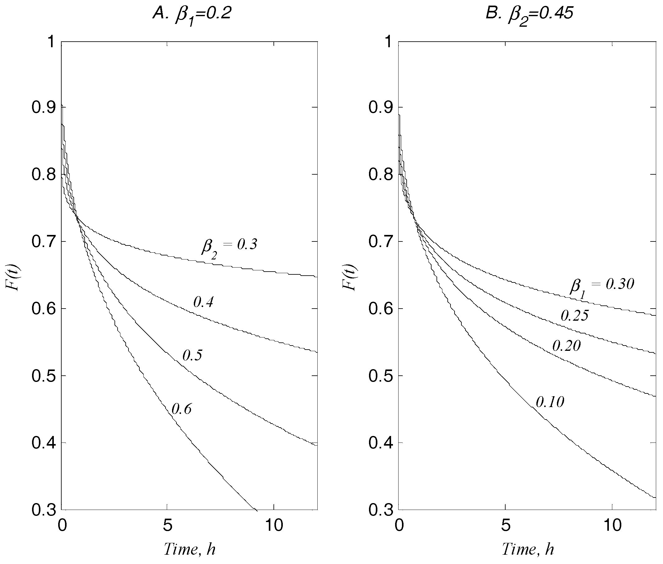
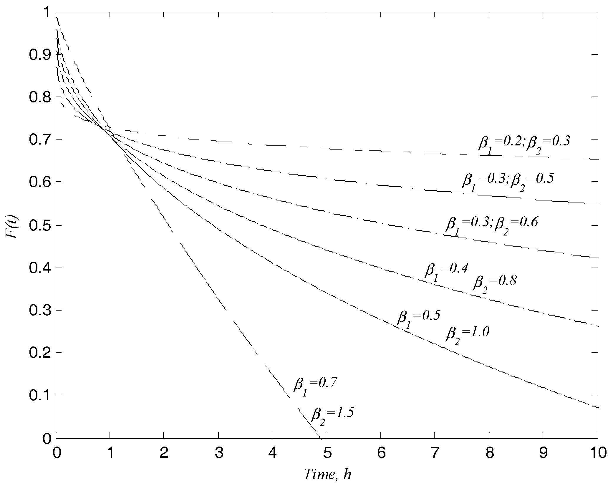
The temporal component of the solutions are illustrated to examine the effect of the model parameters ${\mathsf{\beta }}_2$ and ${\mathsf{\beta }}_1$ on flow processes which are shown to explain realistic physical processes.

The presentations here and earlier [1] include the convection term due to gravity, $\frac{\partial K(\mathsf{\theta })}{\partial \left|z\right|}$ for non-swelling soils and $\frac{\partial K(\mathsf{\theta })}{\partial \left|m\right|}$ for swelling soils. Due to the fact that the diffusivity, $D(\mathsf{\theta })$, and the hydraulic conductivity, $K(\mathsf{\theta })$, are related functions [1], the fractional connections between $D(\mathsf{\theta })$ and $K(\mathsf{\theta })$ are more complex which need to be explored. In the present case, a constant diffusivity and hydraulic conductivity are used and, with functions for $D(\mathsf{\theta })$ and $K(\mathsf{\theta })$, the fPDE with a fractional term $\frac{{\partial }^{\mathsf{\eta }}K(\mathsf{\theta })}{\partial {\left|z\right|}^{\mathsf{\eta }}}$ or $\frac{{\partial }^{\mathsf{\eta }}K(\mathsf{\theta })}{\partial {\left|m\right|}^{\mathsf{\eta }}}$ with $0<\eta <1$ needs to be explored.

For a general background to fractional calculus, its applications, and the methods for solutions as well as related topics, the reader is referred to other sources [2,3,6,12,15,21,26,27,28,29]. While more details of the fPDE-based models are being explored and refined, there is a need to develop methods for estimating the parameters in the models for unsaturated flow using data from both laboratory and field measurements, and the method suggested in [30] for deriving the conductivity from the fractional boundary-value problem is one option. Detailed methods for estimating these parameters are beyond the scope of this paper.

References

1. Su, N. Mass-time and space-time fractional partial differential equations of water movement in soils: Theoretical framework and application to infiltration. J. Hydrol. 2014, 519, 1792–1803. [Google Scholar] [CrossRef]
2. Gorenflo, R.; Mainardi, F. Simply and multiply scaled diffusion limits for continuous time random walks. J. Phys. Conf. Ser. 2005, 7, 1–16. [Google Scholar] [CrossRef]
3. Gorenflo, R.; Mainardi, F.; Vivoli, A. Continuous-time random walk and parametric subordination in fractional diffusion. Chaos Solitons Fractals 2007, 34, 87–103. [Google Scholar] [CrossRef]
4. Bochner, S. Diffusion equation and stochastics processes. Proc. Nat. Acad. Sci. USA 1949, 35, 368–370. [Google Scholar] [CrossRef] [PubMed]
5. Saichev, A.; Zaslavsky, D. Fractional kinetic equations: solutions and applications. Chaos 1949, 7, 753–764. [Google Scholar] [CrossRef] [PubMed]
6. Zaslavsky, G.M. Chaos, fractional kinetics, and anomalous transport. Phys. Rep. 2002, 371, 461–580. [Google Scholar] [CrossRef]
7. Barenblatt, G.I.; Zheltov, I.; Kochina, I. Basic concepts in the theory of seepage of homogeneous liquids in fissured rocks. J. Appl. Math. Mech. 1960, 24, 852–864. [Google Scholar] [CrossRef]
8. Crofton, M.W. Question 1773. In Mathematical Questions with Their Solutions from the Educational Times; Springer: Berlin, Germany, 1866; Volume 4, pp. 71–72. [Google Scholar]
9. Pearson, K. The problem of the random walk. Nature 1905, 72, 294. [Google Scholar] [CrossRef]
10. Saffman, P.G. A theory of dispersion in a porous medium. J. Fluid Mech. 1959, 6, 321–349. [Google Scholar] [CrossRef]
11. Cox, D.R. Renewal Theory; Methuen: London, UK, 1967. [Google Scholar]
12. Meerschaert, M.M. Fractional Calculus, Anomalous diffusion, and Probability. In Fractional Calculus, Anomalous Diffusion and Probability; Metzler, R., Lim, S.C., Klafter, J., Eds.; World Scientific: Singapore, 2011; pp. 265–284. [Google Scholar]
13. Hadid, S.B.; Luchko, Y.F. An operational method for solving fractional differential equations of an arbitrary order. Panamer. Math. J. 1996, 6, 57–73. [Google Scholar]
14. Jiang, H.; Liu, F.; Turner, I.; Burrage, K. Analytical solutions for the multi-term time-space Caputo-Riesz fractional advection-diffusion equations on a finite domain. J. Math. Anal. Appl. 2012, 389, 1117–1127. [Google Scholar] [CrossRef] [Green Version]
15. Schumer, R.; Benson, D.A.; Meerschart, M.M.; Baeumer, B. Fractal mobile-immobile solute transport. Water Resour. Res. 2003, 39, 1–12. [Google Scholar] [CrossRef]
16. Su, N. Distributed-order infiltration, absorption and water exchange in mobile and immobile zones of swelling soils. J. Hydrol. 2012, 468–469, 1–10. [Google Scholar] [CrossRef]
17. Su, N.; Nelson, P.N.; Connor, S. The distributed-order fractional-wave equation of groundwater flow: Theory and application to pumping and slug tests. J. Hydrol. 2015, 529, 1263–1273. [Google Scholar] [CrossRef]
18. Smiles, D.E.; Rosenthal, M.J. The movement of water in swelling materials. Aust. J. Soil Res. 1968, 6, 237–248. [Google Scholar] [CrossRef]
19. Philip, J.R. Hydrostatics and hydrodynamics in swelling soils. Water Resour. Res. 1969, 5, 1070–1077. [Google Scholar] [CrossRef]
20. Gorenflo, R.; Mainardi, F. Parametric Subordination in Fractional Diffusion Processes. In Fractional Dynamics, Recent Advances; Klafter, J., Lim, S.C., Metzler, R., Eds.; World Scientific: Singapore, 2011; pp. 227–261. [Google Scholar]
21. Zhang, Y.; Benson, D.A.; Reeves, D.M. Time and space nonlocalities underlying fractional-derivative models: Distribution and literature review of field applications. Adv. Water Resour. 2009, 32, 561–581. [Google Scholar] [CrossRef]
22. Chechkin, A.; Gorenflo, R.; Sokolov, I.M. Retarding subdiffusion and acceleration superdiffusion governed by distributed-order fractional diffusion equation. Phys. Rev. E. 2002, 66, 046129. [Google Scholar] [CrossRef] [PubMed]
23. Bronshtein, I.N.; Semendyayev, K.A. Handbook of Mathematics; Verlag Harri Deutsch, Van Nostrand Reinhold Co.: New York, NY, USA, 1979. [Google Scholar]
24. Philip, J.R. On solving the unsaturated flow equations: The flux-concentration relation. Soil Sci. 1973, 116, 328–335. [Google Scholar] [CrossRef]
25. Smith, R.E.; Smettem, K.R.J.; Broadbridge, P.; Woolhiser, D.A. Infiltration Theory for Hydrologic Applications; AGU: Washington, DC, USA, 2002. [Google Scholar]
26. Cushman, J.H.; Ginn, T.R. Fractional advection-dispersion equation: A classical mass balance with convolution-Fickian flux. Water Resour. Res. 2000, 36, 3763–3766. [Google Scholar] [CrossRef]
27. Ma, W.X.; Huang, T.; Zhang, Y. A multiple exp-function method for nonlinear differential equations and its application. Phys. Scr. 2010, 82, 065003. [Google Scholar] [CrossRef]
28. Ma, W.X.; Fuchssteiner, B. Explicit and exact solutions to a Kolmogorov-Petrovskii-Piskunov equation. Int. J. Nonl. Mech. 1996, 31, 329–338. [Google Scholar] [CrossRef]
29. Bucur, C.; Valdinoci, E. Nonlocal Diffusion and Applications. In Lecture Notes of the Unione Matematica Italiana; Springer: Bologna, Italy, 2010; p. 155. [Google Scholar]
30. Ochoa-Tapia, J.A.; Valdes-Parada, F.J.; Alvarez-Ramirez, J. A fractional-order Darcy’s law. Physica A 2007, 374, 1–14. [Google Scholar] [CrossRef]
31. Umarov, S.; Gorenflo, R. On multi-dimensional random walk models approximating symmetric space-time-fractional diffusion processes. Fract. Calc. Appl. Anal. 2005, 8, 73–88. [Google Scholar]
32. Bhalekar, S.; Daftardar-Gejji, V. Corridendum. Appl. Math. Comput. 2013, 219, 8413–8415. [Google Scholar]
33. Gradshteyn, I.S.; Ryzhik, I.M. Table of Integrals, Series, and Products; Academic: San Diego, CA, USA, 1994. [Google Scholar]
34. Podlubny, I. Fractional Differential Equations; Academic Press: San Diego, CA, USA, 1999. [Google Scholar]
Figure 1. Moisture distributions affected by the orders of fractional derivatives in Equation (14). (A): Fixed β 1 with variable β 2 indicating the facilitating role of β 2 in large pores; (B): fixed β 2 with variable β 1 indicating the trapping role of β 1 in small pores. In both cases, the joint parameter is K 1 = 0.01 .
Hydrology 04 00008 g001
Figure 2. The facilitating role of β 2 overtaking β 1 in increasing the flow rate when both orders increase. The illustration of Equation (14) with pairs of β 2 and β 1 (the joint parameter K 1 = 0.01 ).
Hydrology 04 00008 g002