
Application of HEC-HMS in a Cold Region Watershed and Use of RADARSAT-2 Soil Moisture in Initializing the Model


Abstract
:1. Introduction
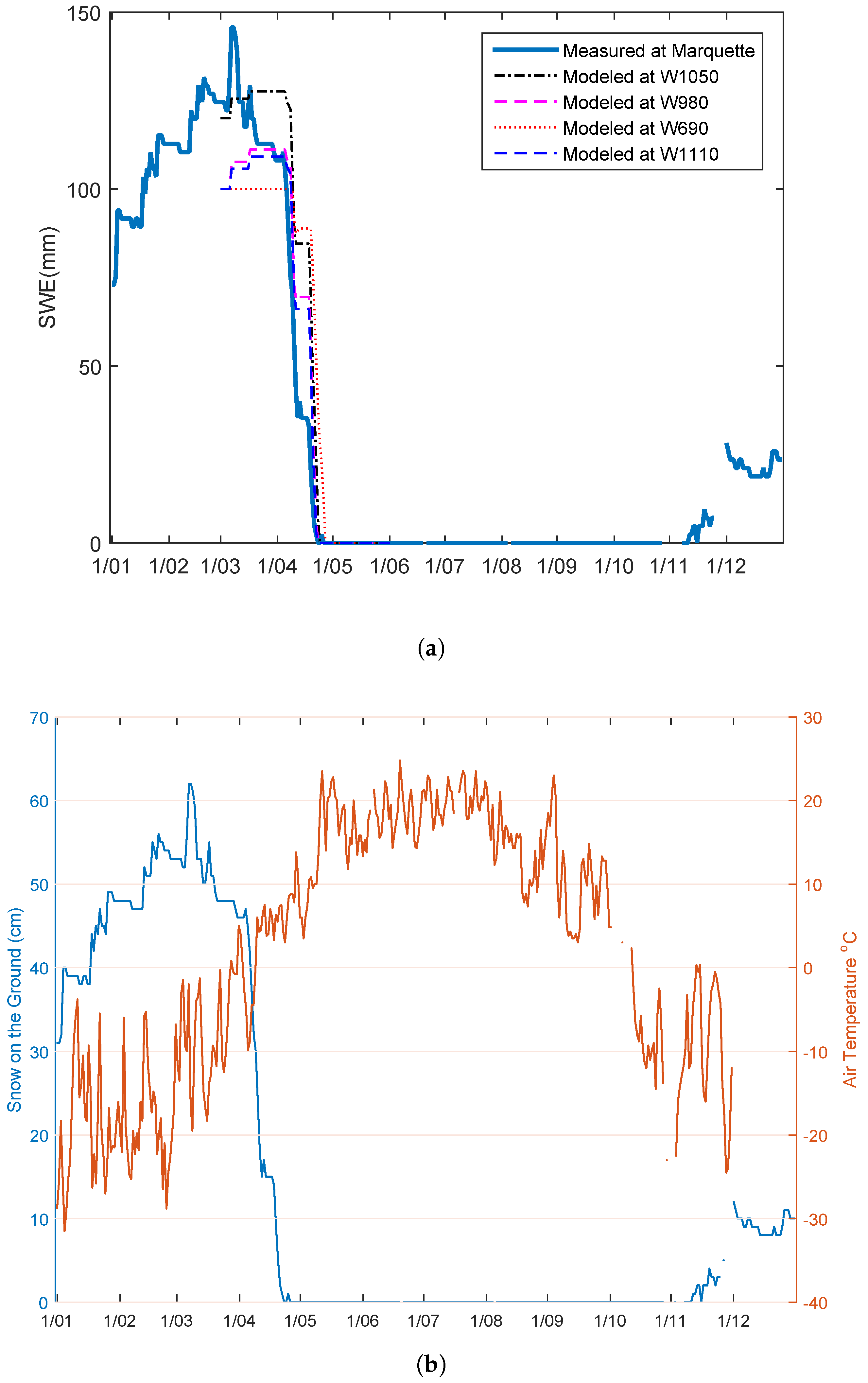
- (a)
- to assess the usability/applicability and potential benefits of HEC-HMS using RADARSAT-2-derived soil moisture estimates in the snowmelt-dominated Sturgeon Creek watershed and;
- (b)
- to test the sensitivity of initial soil moisture in setting the HEC-HMS model for flood forecasting.
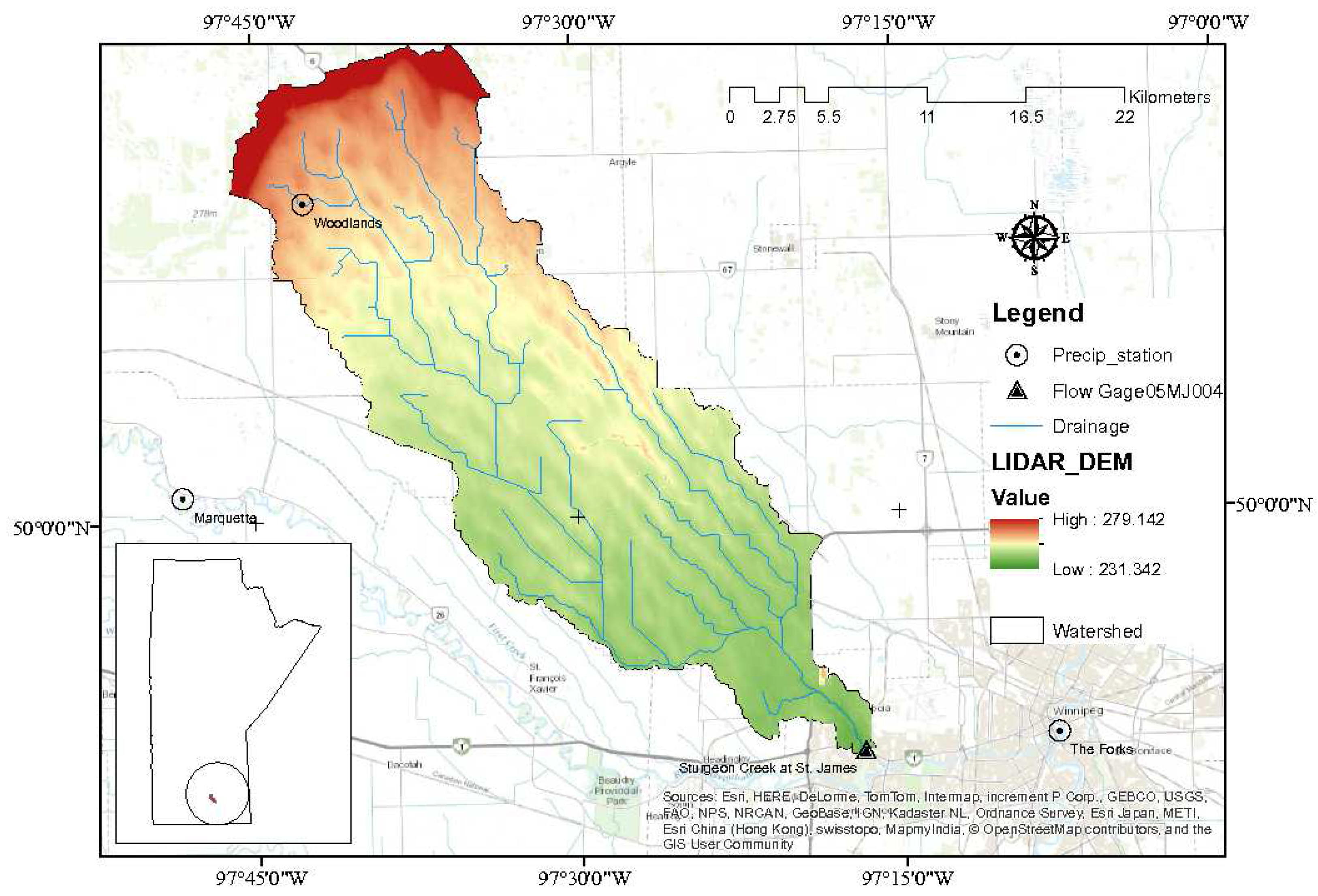
2. Study Area and Data
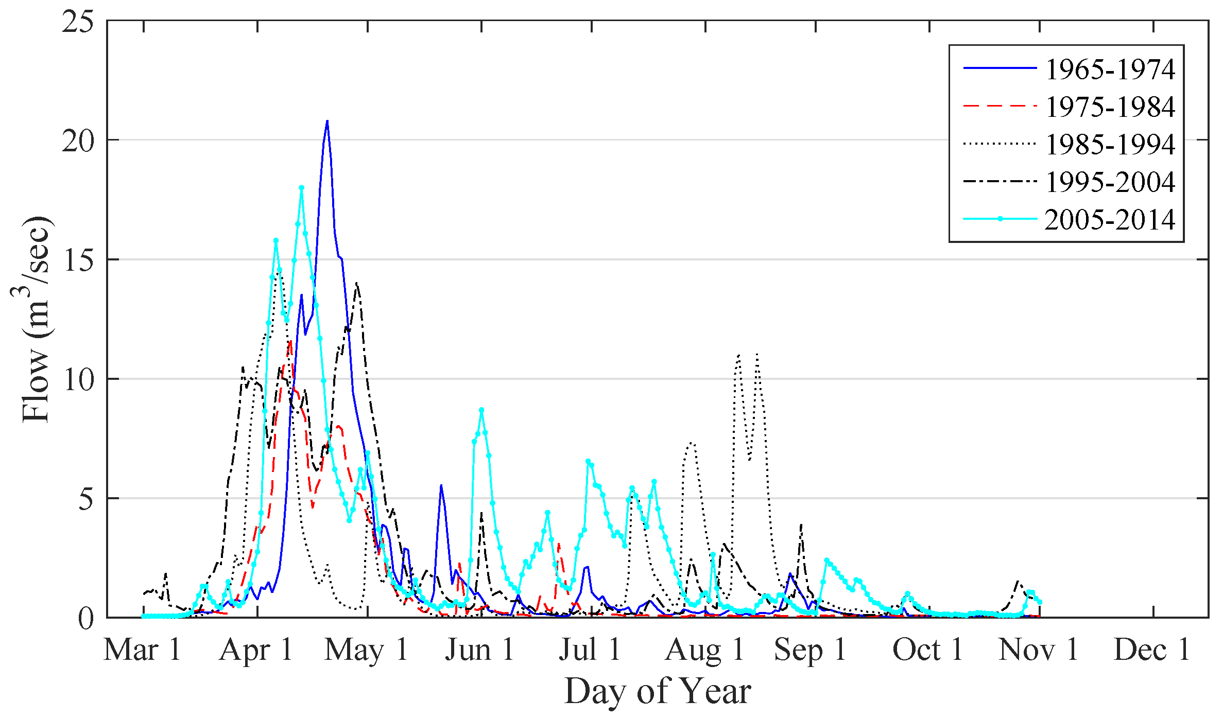
2.1. Flow Data
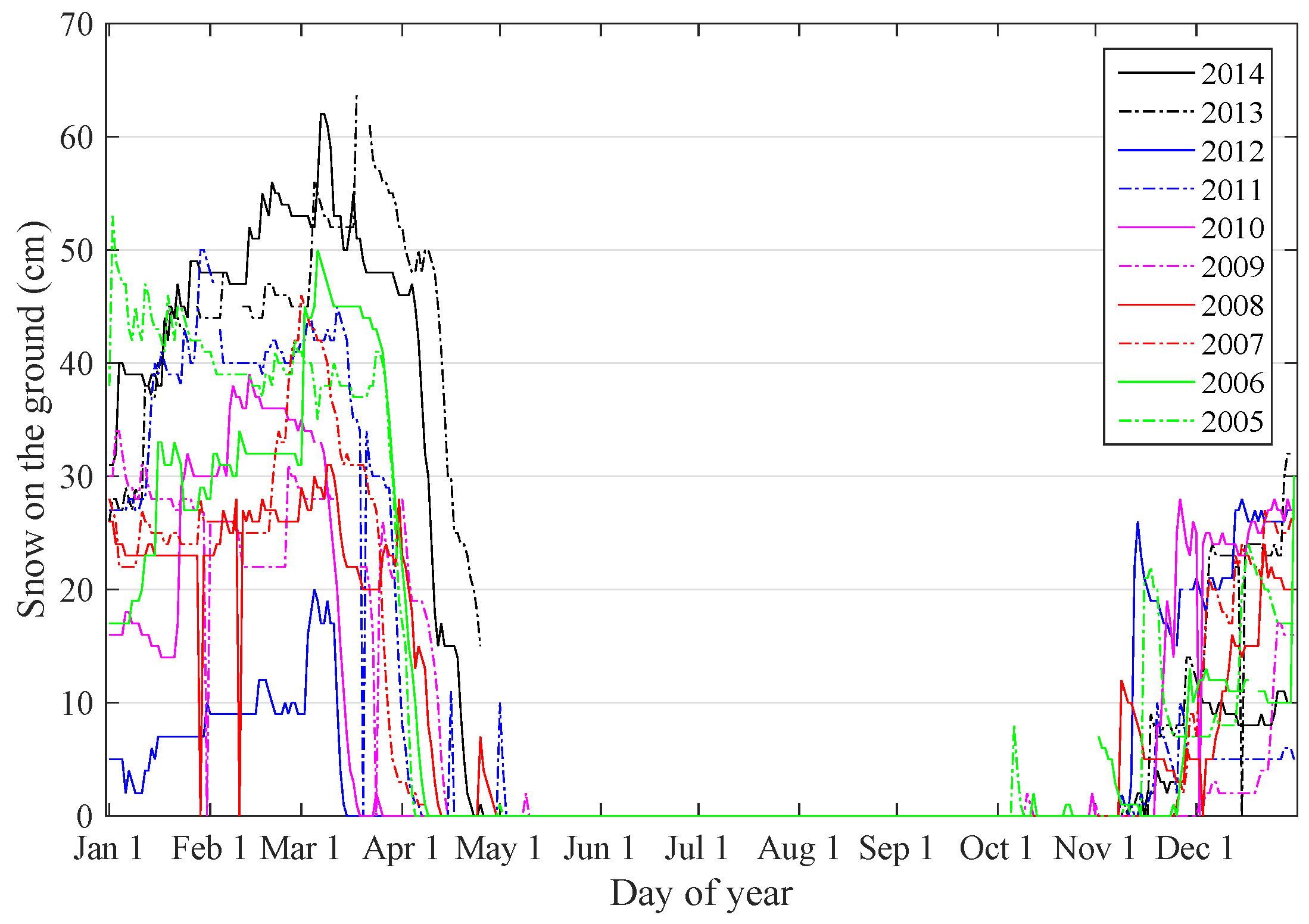
2.2. Weather Data
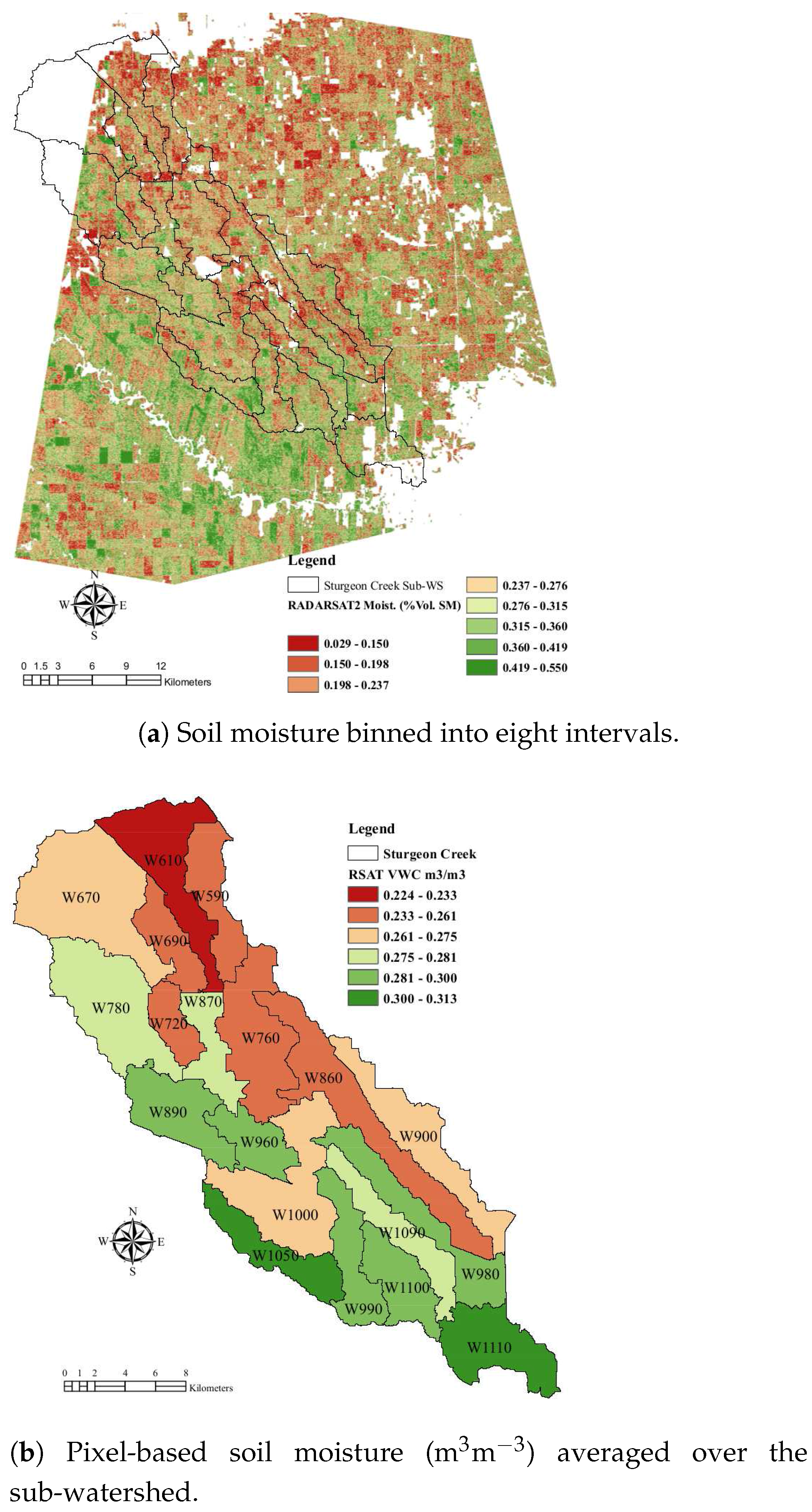
2.3. Soil Moisture Estimates from RADARSAT-2 Satellite Data
2.4. Fall Soil Moisture Survey Data
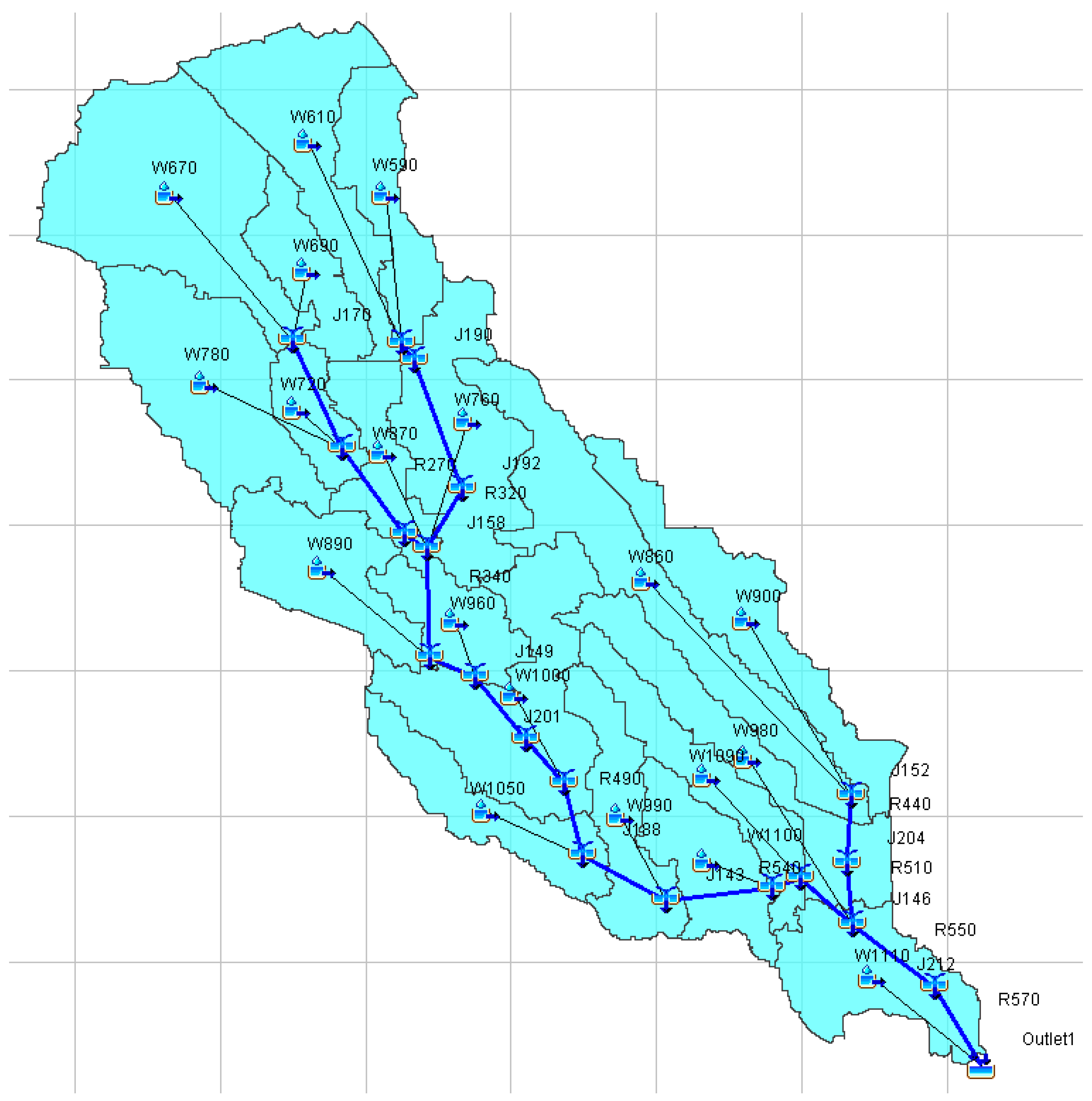
3. HEC-HMS Model
3.1. Model Evaluation
4. Results and Discussion
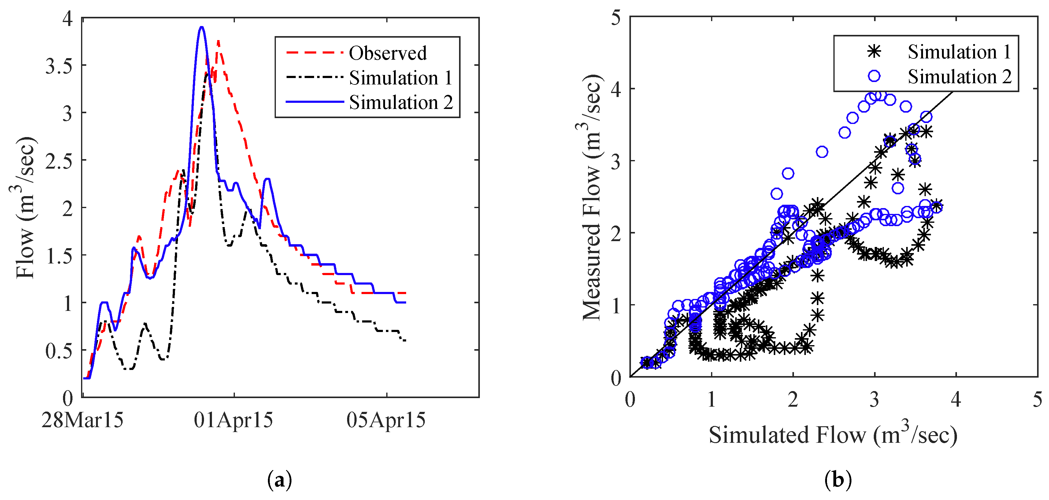
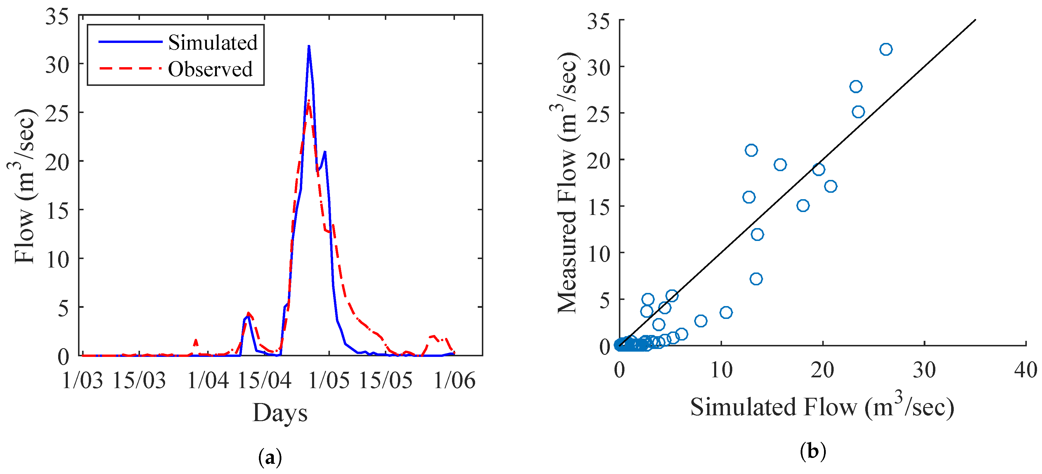
4.1. Event Modelling
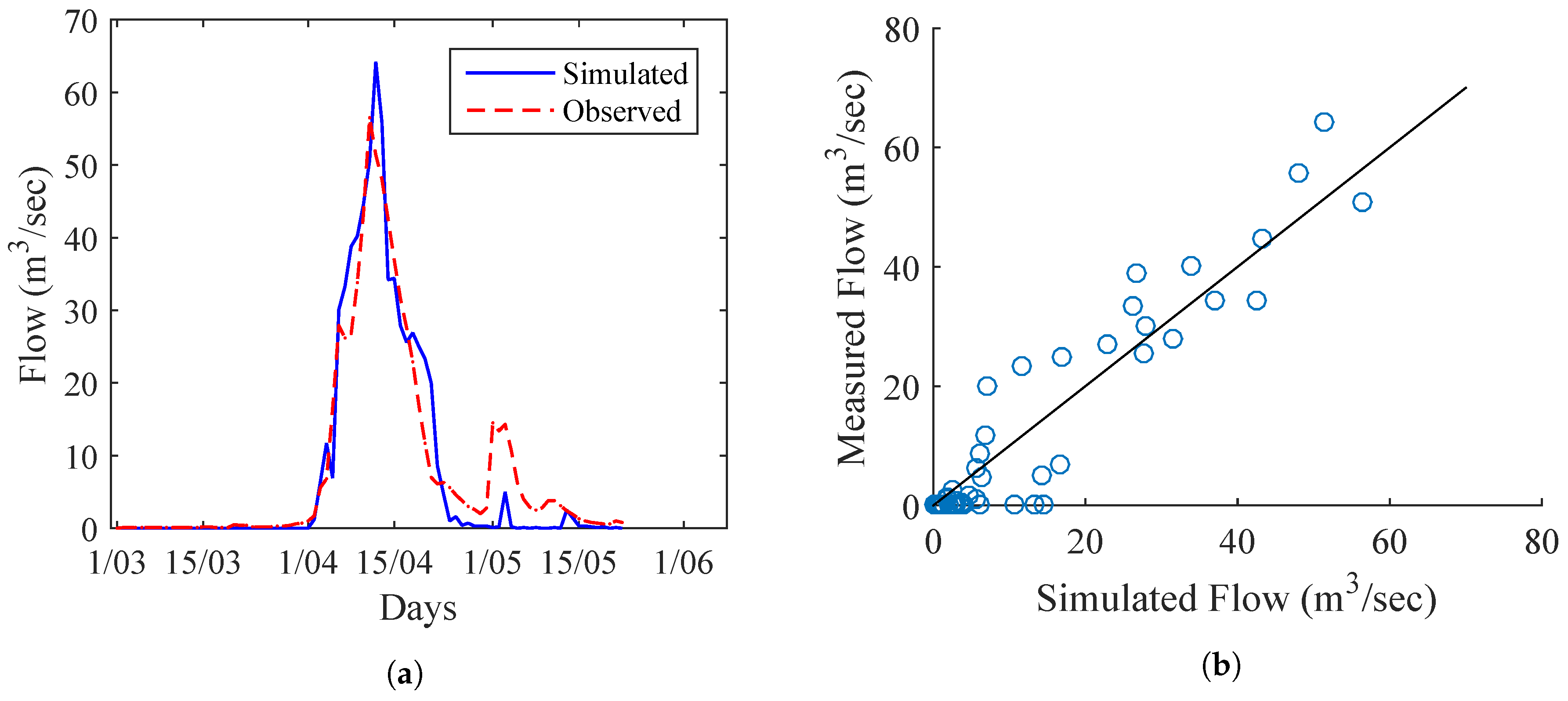
4.2. Continuous Modelling
4.3. Snowmelt Model
4.3.1. Sensitivity of SMA Parameters
4.3.2. Initial Soil Moisture
5. Conclusions
Acknowledgments
Author Contributions
Conflicts of Interest
Abbreviations
| AAFC | Agriculture and Agri-Food Canada |
| ECC | Environment and Climate Change Canada |
| MA | Manitoba Agriculture |
| SAR | Synthetic aperture radar |
| RADARSAT | Canadian remote sensing Earth observation satellite |
| HEC-HMS | Hydrologic Modelling System developed by the Hydrologic Engineering Center |
| SMA | Soil moisture accounting |
| MANAPI | Manitoba Antecedent Precipitation Index model |
| WSC | Water Survey Canada |
| HFC | Hydrologic Forecast Center |
| DEM | Digital elevation model |
| LiDAR | Light detection and ranging |
| IEM | Integral equation model |
| HH | Backscatter horizontal transmission and horizontal receive |
| VV | Backscatter vertical transmission and vertical receive |
| SCS | Soil Conservation Service |
| SWE | Snow water equivalent |
References
- Blais, E.L.; Clark, S.; Dow, K.; Ranniec, B.; Stadnyk, T.; Wazney, L. Background to flood control measures in the Red and Assiniboine River Basins. Can. Water Resour. J. 2015. [Google Scholar] [CrossRef]
- Flood Review Task Force. Manitoba 2011 Flood Review Task Force Report. Report to the Minister of Manitoba Infrastructure and Transportation, 2013. Available online: https://www.gov.mb.ca/asset_library/en/2011flood/flood_review_task_force_report.pdf (accessed on 7 April 2016).
- Rannie, W. The 1997 flood event in the Red River basin: Causes, assessment and damages. Can. Water Resour. J. 2015. [Google Scholar] [CrossRef]
- Stadnyk, T.; Dow, K.; Wazney, L.; Blais, E.L. The 2011 flood event in the Red River Basin: Causes, assessment and damages. Can. Water Resour. J. 2015, 65–73. [Google Scholar] [CrossRef]
- Bower, S.S. Natural and unnatural complexities: Flood control along Manitoba’s Assiniboine River. J. Hist. Geogr. 2010, 36, 57–67. [Google Scholar] [CrossRef]
- Rasmussen, P.F. Evaluation of Flood Forecasting and Warning SSystem in Canada. 22nd Canadian Hyrotechnical Conference, 2015. Available online: http://www.nsercfloodnet.ca/files/Track_5_-_Presentation_-_Flood_forecasting_in_Canada_CSCE_2015.pdf (accessed on 7 April 2016).
- Steenbergen, N.V.; Willems, P. Rainfall uncertainty in flood forecasting: Belgian case study of rivierbeek. J. Hydrol. Eng. 2014, 19. [Google Scholar] [CrossRef]
- Dietrich, J.; Schumann, A.H.; Redetzky, M.; Walther, J.; Denhard, M.; Wang, Y.; Pfutzner, B.; Büttner, U. Assessing uncertainties in flood forecasts for decision making: prototype of an operational flood management system integrating ensemble predictions. Nat. Hazards Earth Syst. Sci. 2009, 9, 1529–1540. [Google Scholar] [CrossRef]
- Brocca, L.; Melone, F.; Moramarco, T.; Wagner, W.; Naeimi, V.; Bartalis, Z.; Hasenauer, S. Improving runoff prediction through the assimilation of the ASCAT soil moisture product. Hydrol. Earth Syst. Sci. 2010, 14, 1881–1893. [Google Scholar] [CrossRef]
- Sutanudjaja, E.H.; van Beek, L.P.H.; de Jong, S.M.; van Geer, F.C.; Bierkens, M.F.P. Calibrating a large-extent high-resolution coupled groundwater-land surface model using soil moisture and discharge data. Water Resour. Res. 2014, 50, 687–705. [Google Scholar] [CrossRef]
- Tramblay, Y.; Bouaicha, R.; Brocca, L.; Dorigo, W.; Bouvier, C.; Camici, S.; Servat, E. Estimation of antecedent wetness conditions for flood modelling in northern Morocco. Hydrol. Earth Syst. Sci. 2012, 16, 4375–4386. [Google Scholar] [CrossRef]
- Li, Y.; Grimaldi, S.; Walker, J.P.; Pauwels, V.R.N. Application of Remote Sensing Data to Constrain Operational Rainfall-Driven Flood Forecasting: A Review. Remote Sens. 2016, 8. [Google Scholar] [CrossRef]
- Massari, C.; Brocca, L.; Barbetta, S.; Papathanasiou, C.; Mimikou, M.; Moramarco, T. Using globally available soil moisture indicators for flood modelling in Mediterranean catchments. Hydrol. Earth Syst. Sci. 2014, 18, 839–853. [Google Scholar] [CrossRef] [Green Version]
- Xu, X.; Li, J.; Tolson, B.A. Progress in integrating remote sensing data and hydrologic modeling. Appl. Meteorol. Climatol. 2014, 87, 61–77. [Google Scholar] [CrossRef]
- McNairn, H.; Merzouki, A.; Pacheco, A. Estimating surface soil moisture ubing RADARSAT-2. In International Archives of the Photogrammetry, Remote Sensing and Spatial Information Science; Copernicus GmbH: Göttingen, Germany, 2010; pp. 576–579. [Google Scholar]
- AAFC Information Bulletin 99-4. In Soils and Terrain. An Introduction to the Land Resource. Rural Municipality of Rosser. Information Bulletin 99-4; Technical Report; Land Resources Unit, Brandon Research Centre, Research Branch, Agriculture and Agri-Food Canada: Winnipeg, MB, Canada, 1999.
- AECOM Canada. Sturgeon Creek Hydrodynamic Model and Economic Study, Project No.: F685 003 00 (4.6.1); Technical Report; Water Stewardship, Government of Canada: Winnipeg, MB, Canada, 2009.
- Jacob, D.; Lorenz, P. Future trends and variability of the hydhydrologic cycle in different IPCC SRES emission scenarios—A case study for the Baltic Sea Region. Boreal Environ. Res. 2009, 14, 100–113. [Google Scholar]
- Thornthwaite, C.W. An Approach toward a Rational Classification of Climate. Geogr. Rev. 1948, 38, 55–94. [Google Scholar] [CrossRef]
- Feldman, A.D. Hydrologic Modeling System HEC-HMS, Technical Reference Manual; U.S. Army Corps of Engineers, Hydrologic Engineering Center HEC: Davis, CA, USA, 2000. [Google Scholar]
- Alvarez, J.; Verhoest, N.E.C.; Casali, J.; Gonzalez-Audicana, M.; Lopez, J.J. RADARSAT based surface soil moisture retrieval on agricultural catchments of Navarre (Spain). In Proceedings of the 2004 IEEE International Geoscience and Remote Sensing Symposium, Anchorage, AK, USA, 20-24 September 2004; Volume 5, pp. 3507–3510.
- Merzouki, A.; McNairn, H. A Hybrid (Multi-Angle and Multipolarization) Approach to Soil Moisture Retrieval Using the Integral Equation Model: Preparing for the RADARSAT Constellation Mission. Can. J. Remote Sens. 2015, 41, 349–362. [Google Scholar] [CrossRef]
- Eilers, P. Sturgeon Creek Soil Moisture Monitoring Stations (SMMS); Soil and Landscape Classification; Contract Number 3000528851. Technical Report; Science and Technology Branch, Agriculture and Agri-Food Canada: Winnipeg, Manitoba, 2013. [Google Scholar]
- Schaffenberg, W.A. Hydrologic Modeling System HEC-HMS, User Manual: Version 4.0; U.S. Army Corps of Engineers, Hydrologic Engineering Center HEC: 609 Second Street, Davis, CA, USA, 2013. [Google Scholar]
- U.S. Army Corps of Engineers. Hydrologic Modeling System (HEC-HMS) Application Guide: Version 4.0; Institute for Water Resources, Hydrologic Engineering Center: Devis, CA, USA, 2015. [Google Scholar]
- Knebl, M.; Yang, Z.L.; Hutchison, K.; Maidment, D. Regional scale flood modeling using NEXRAD rainfall, GIS, and HEC-HMS/RAS: A case study for the San Antonio River Basin Summer 2002 storm event. J. Environ. Manag. 2005, 75, 325–336. [Google Scholar] [CrossRef] [PubMed]
- Du, J.; Qian, L.; Rui, H.; Zuo, T.; Zheng, D.; Xu, Y.; Xu, C.Y. Assessing the effects of urbanization on annual runoff and flood events using an integrated hydrological modeling system for Qinhuai River basin, China. J. Hydrol. 2012, 464–465, 127–139. [Google Scholar] [CrossRef]
- Haberlandt, U.; Radtke, I. Hydrological model calibration for derived flood frequency analysis using stochastic rainfall and probability distributions of peak flows. Hydrol. Earth Syst. Sci. 2014, 18, 353–365. [Google Scholar] [CrossRef] [Green Version]
- Fleming, M.; Neary, V. Continuous hydrologic modeling study with the hydrologic modeling system. ASCE J. Hydrol. Eng. 2004, 9, 175–183. [Google Scholar] [CrossRef]
- Gebre, S.L. Application of the HEC-HMS model for runoff simulation of upper blue Nile River Basin. Hydrol. Curr. Res. 2015, 6, 1–8. [Google Scholar] [CrossRef]
- Singh, W.R.; Jain, M.K. Continuous Hydrological Modeling using Soil Moisture Accounting Algorithm in Vamsadhara River Basin, India. J. Water Res. Hydraul. Eng. 2015, 4, 398–408. [Google Scholar] [CrossRef]
- Gyawali, R.; Watkins, D.W. Continuous Hydrologic Modeling of Snow-Affected Watersheds in the Great Lakes Basin Using HEC-HMS. ASCE J. Hydrol. Eng. 2013, 18, 29–39. [Google Scholar] [CrossRef]
- Hall, M.J. How well does your model fit the data? J. Hydroinf. 2001, 3, 49–55. [Google Scholar]
- Krause, P.; Boyle, D.P.; Base, F. Comparison of different efficiency criteria for hydrological model assessment. Adv. Geosci. 2005, 5, 89–97. [Google Scholar] [CrossRef]
- Bardsley, W.E. A goodness of fit measure related to r2 for model performance assessment. Hydrol. Process. 2013, 27, 2851–2856. [Google Scholar] [CrossRef] [Green Version]
- Nash, J.E.; Sutcliffe, J.V. River flow forecasting through conceptual models part I–A discussion of principles. J. Hydrol. 1970, 10, 282–290. [Google Scholar] [CrossRef]
- Henriksen, H.J.; Troldborg, L.; Nyegaard, P.; Sonnenborg, T.O.; Refsgaard, J.C.; Madsen, B. Methodology for construction, calibration and validation of a national hydrological model for Denmark. J. Hydrol. 2003, 280, 52–71. [Google Scholar] [CrossRef]
- Legates, D.R.; McCabe, G.J. Evaluating the use of goodness-of-fit measures in hydrologic and hydroclimatic model validation. Water Resour. Res. 1999, 35, 233–241. [Google Scholar] [CrossRef]
- Moriasi, D.N.; Arnold, J.G.; Liew, M.W.V.; Bingner, R.L.; Harmel, R.D.; Veith, T.L. Model evaluation guidelines for systematic quantification of accuracy in watershed simulations. Am. Soc. Agric. Biol. Eng. 2007, 50, 885–900. [Google Scholar]
- Sturm, M.; Taras, B.; Liston, G.E.; Derksen, C.; Jonas, T.; Lea, J. Estimating snow water equivalant using snow depth data and climate classes. J. Hydrometeorol. 2010, 11, 1380–1394. [Google Scholar] [CrossRef]
- Theil, H. A rank-invariant method of linear and polynomial regression analysis, I, II, III. In Proceedings of the Royal Netherlands Academy of Sciences, Amsterdam, the Netherlands, 30 September 1950; pp. 1397–1412.
- Sen, P.K. Estimates of the regression coefficient based on Kendall’s tau. J. Am. Stat. Assoc. 1968, 63, 1379–1389. [Google Scholar] [CrossRef]
- Roy, D.; Begam, S.; Ghosh, S.; Jana, S. Calibration and validation of HEC-HMS model for a river basin in Eastern India. J. Eng. Appl. Sci. 2013, 8, 40–56. [Google Scholar]
- Czigany, S.; Pirkhoffer, E.; Geresdi, I. Impact of extreme rainfall and soil moisture on flash flood generation. J. Hung. Meteorol. Serv. 2010, 114, 79–100. [Google Scholar]
- Hegedus, P.; Czigany, S.; Balatonyi, L.; Pirkhoffer, E. Analysis of soil boundary conditions of flash Floods in a small basin in SW Hungary. Cent. Eur. J. Geosci. 2013, 5, 97–111. [Google Scholar] [CrossRef]


| Basin Model | Meteorological Model | ||
|---|---|---|---|
| Parameter Method | Selected Method | Parameter Method | Selected Method |
| Canopy | Simple Canopy | Precipitation | Inverse Distance |
| Surface | Simple Surface | Evaporation | Monthly Average |
| Transform | SCS Unit Hydrograph | Snowmelt | Temperature Index |
| Base Flow | Recession | Shortwave | None |
| Routing | Muskingum | ||
| Loss | Soil Moisture Accounting | ||
| Parameter | Unit | Value |
|---|---|---|
| PX Temperature | oC | 1.7847 |
| Base Temperature | oC | 0.6294 |
| Wet Melt Rate | mm/oC-day | 0.9876 |
| Rain Rate Limit | mm/day | 2 |
| ATI -Melt Rate Coefficient | - | 0.9995 |
| Cold Limit | mm/day | 20 |
| ATI-Cold Rate Coefficient | - | 0.9995 |
| Water Capacity | % | 10 |
| Ground Melt | mm/day | 0 |
| Model | Duration | Dev. of Runoff | Nash |
|---|---|---|---|
| Simulation | Volume, D (%) | Co-efficient, N | |
| Event (Simulation 2) | 28 March 2015–6 April 2015 | −4.83 | 0.74 |
| Event (Simulation 1) | 28 March 2015–6 April 2015 | −34.25 | 0.31 |
| Continuous | 01 March 14–1 June 2014 | −17.9 | 0.87 |
| Continuous | 01 March 11–1 June 2011 | −7.22 | 0.88 |
| Percent | Soil | Soil | Tension | Maximum | GW1 | Max Canopy |
|---|---|---|---|---|---|---|
| Deviation | Storage | Percolation | Storage | Infiltration | Storage | Storage |
| (%) | (mm) | (mm) | (mm) | (mm/h) | (mm) | (mm) |
| Sub-Watershed W1100 | ||||||
| 40 | −20.06 | −16.07 | 17.02 | −15.20 | −0.28 | −9.73 |
| 30 | −15.83 | −12.98 | 11.40 | −12.11 | −0.24 | −9.02 |
| 20 | −11.04 | −9.14 | 6.93 | −8.46 | −0.16 | −7.36 |
| 10 | −5.74 | −4.87 | 3.36 | −4.71 | −0.08 | −4.63 |
| 0 | 0.00 | 0.00 | 0.00 | 0.00 | 0.00 | 0.00 |
| −10 | 6.73 | 5.54 | −2.89 | 5.32 | 0.12 | 5.70 |
| −20 | 15.43 | 11.79 | −6.02 | 11.74 | 0.28 | 12.74 |
| −30 | 27.78 | 18.60 | −8.94 | 18.84 | 0.44 | 20.74 |
| −40 | 48.12 | 26.39 | −11.83 | 28.08 | 0.67 | 28.41 |
| Slope (b) | 0.68 | 0.52 | −0.33 | 0.51 | 0.01 | 0.50 |
| Ranking | 1 | 2 | 5 | 3 | 6 | 4 |
| Sub-Watershed W870 | ||||||
| 40 | −16.67 | −11.34 | 5.92 | −8.19 | −0.07 | −6.41 |
| 30 | −12.87 | −8.80 | 4.53 | −6.84 | −0.07 | −2.82 |
| 20 | −8.86 | −5.89 | 3.38 | −4.65 | −0.04 | −1.37 |
| 10 | −4.62 | −3.23 | 1.42 | −2.56 | −0.03 | −0.49 |
| 0 | 0.00 | 0.00 | 0.00 | 0.00 | 0.00 | 0.00 |
| −10 | 5.19 | 3.12 | −0.72 | 3.13 | 0.00 | 0.52 |
| −20 | 10.81 | 6.36 | −1.13 | 8.39 | 0.04 | 4.56 |
| −30 | 17.53 | 10.45 | −1.77 | 14.03 | 0.07 | 9.65 |
| −40 | 25.09 | 13.38 | −2.12 | 21.97 | 0.11 | 12.12 |
| Slope (b) | 0.50 | 0.31 | −0.12 | 0.32 | 0.00 | 0.21 |
| Ranking | 1 | 3 | 5 | 2 | 6 | 4 |
| Sub-Watershed Sensitivity | Watershed Sensitivity | |||||||
|---|---|---|---|---|---|---|---|---|
| Initial Soil | Peak | Diff. | Cum. | Cum. | Peak | Diff. | Cum. | Cum. |
| Moisture | Flow | Peak | Outflow | Flow | Flow | Peak | Outflow | Flow |
| (m/s) | (%) | (1000 m) | Diff. (%) | (m/s) | (%) | (1000 m) | Diff. (%) | |
| Sub-watershed W610, bulk density 1.32 gm/cm | ||||||||
| Calibration; 0.229 | 0.4 | 42.9 | 3.9 | 1097 | ||||
| mm /45.5%. | ||||||||
| 0.326 m m /60% | 0.8 | +100 | 94.6 | +121 | 4.3 | +10 | 1148 | +5 |
| 0.125 m m /25% | 0.1 | −75 | 12.3 | −71 | 3.7 | −5 | 1067 | −3 |
| Sub-watershed W960, bulk density 1.39 gm/cm | ||||||||
| Calibration; 0.291 | 0.8 | 101.1 | 3.9 | 1097 | ||||
| mm /61.1%. | ||||||||
| 0.215 m m /45% | 0.4 | −50 | 51.5 | −49 | 3.8 | −3 | 1048 | −4 |
| 0.125 m m /25% | 0.2 | −75 | 22.9 | −77 | 3.8 | −3 | 1020 | −7 |
| Sub-watershed W1000, bulk density 1.04 gm/cm | ||||||||
| Calibration; 0.243 | 1.1 | 155.3 | 3.9 | 1097 | ||||
| mm /40%. | ||||||||
| 0.364 m m /60% | 1.9 | +73 | 313.8 | +102 | 4.2 | +8 | 1254 | +14 |
| 0.151 m m /25% | 0.5 | −55 | 67.5 | −57 | 3.8 | −3 | 1010 | −8 |
© 2017 by the authors; licensee MDPI, Basel, Switzerland. This article is an open access article distributed under the terms and conditions of the Creative Commons Attribution (CC BY) license (http://creativecommons.org/licenses/by/4.0/).
Share and Cite
Bhuiyan, H.A.K.M.; McNairn, H.; Powers, J.; Merzouki, A. Application of HEC-HMS in a Cold Region Watershed and Use of RADARSAT-2 Soil Moisture in Initializing the Model. Hydrology 2017, 4, 9. https://doi.org/10.3390/hydrology4010009
Bhuiyan HAKM, McNairn H, Powers J, Merzouki A. Application of HEC-HMS in a Cold Region Watershed and Use of RADARSAT-2 Soil Moisture in Initializing the Model. Hydrology. 2017; 4(1):9. https://doi.org/10.3390/hydrology4010009
Chicago/Turabian StyleBhuiyan, Hassan A. K. M., Heather McNairn, Jarrett Powers, and Amine Merzouki. 2017. "Application of HEC-HMS in a Cold Region Watershed and Use of RADARSAT-2 Soil Moisture in Initializing the Model" Hydrology 4, no. 1: 9. https://doi.org/10.3390/hydrology4010009