
Evaluation of Satellite-Derived Rainfall Estimates for an Extreme Rainfall Event over Uttarakhand, Western Himalayas

 ,
, 
Abstract
:1. Introduction
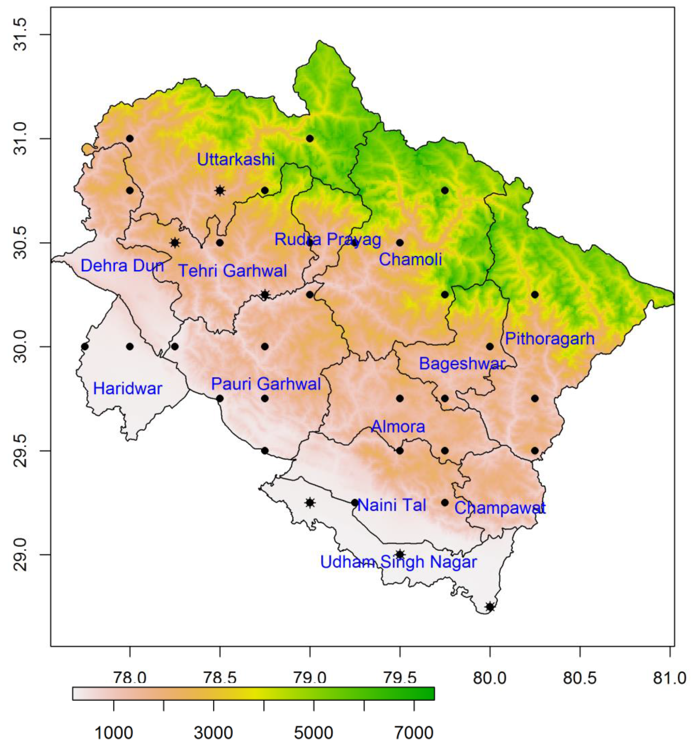
2. Study Area
3. Materials and Methods
3.1. TMPA-3B42 Rainfall Data
3.2. NOAA CPC Morphing Technique (CMORPH) Rainfall Data
3.3. JAXA (GSMaP) Rainfall Data
3.4. India Meteorological Department (IMD) Rainfall Data
3.5. Wadia Institute of Himalayan Geology (WIHG) Daily Discharge and Rainfall Data
3.6. Other Ancillary Data
3.7. Methods
4. Results
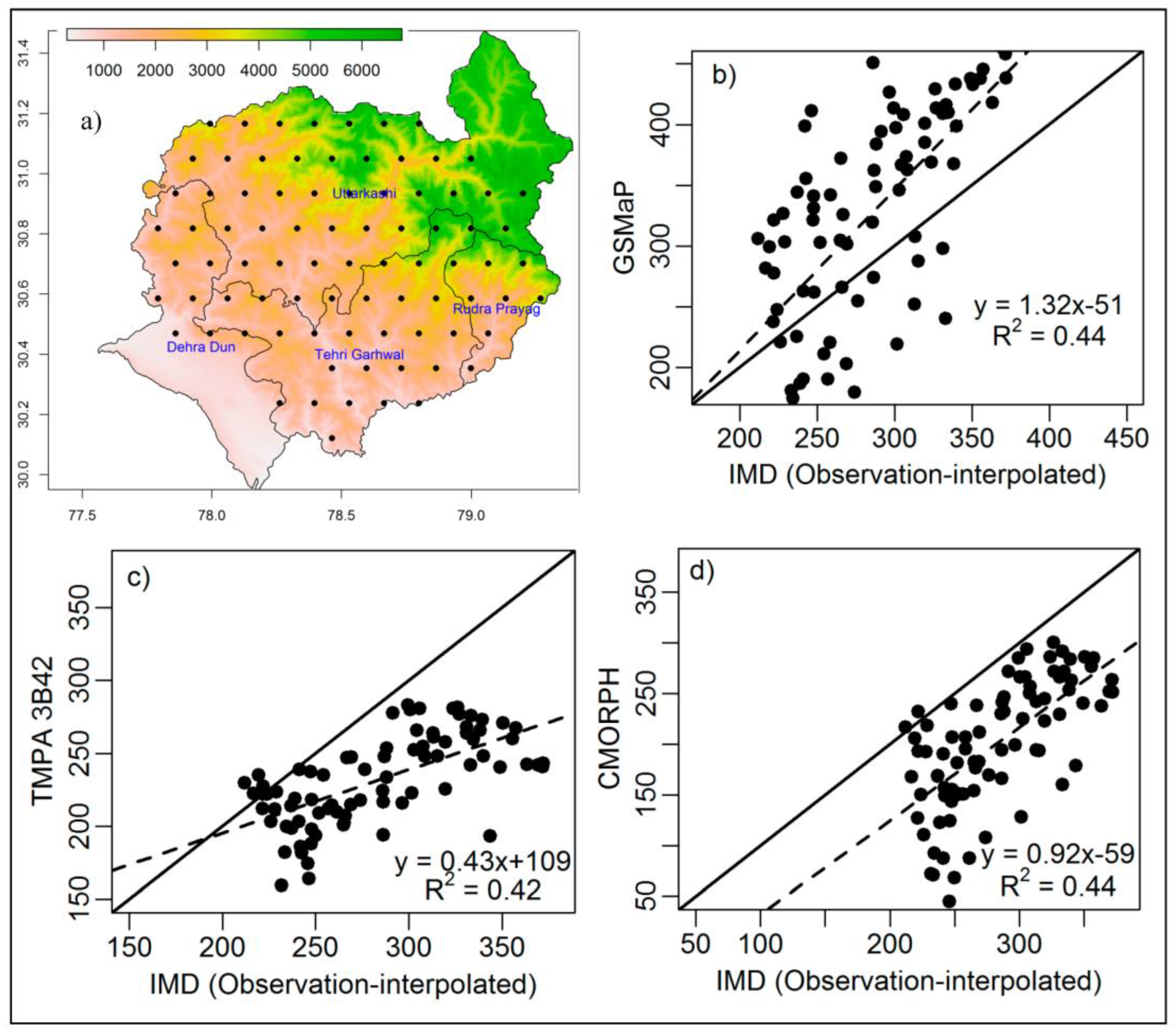
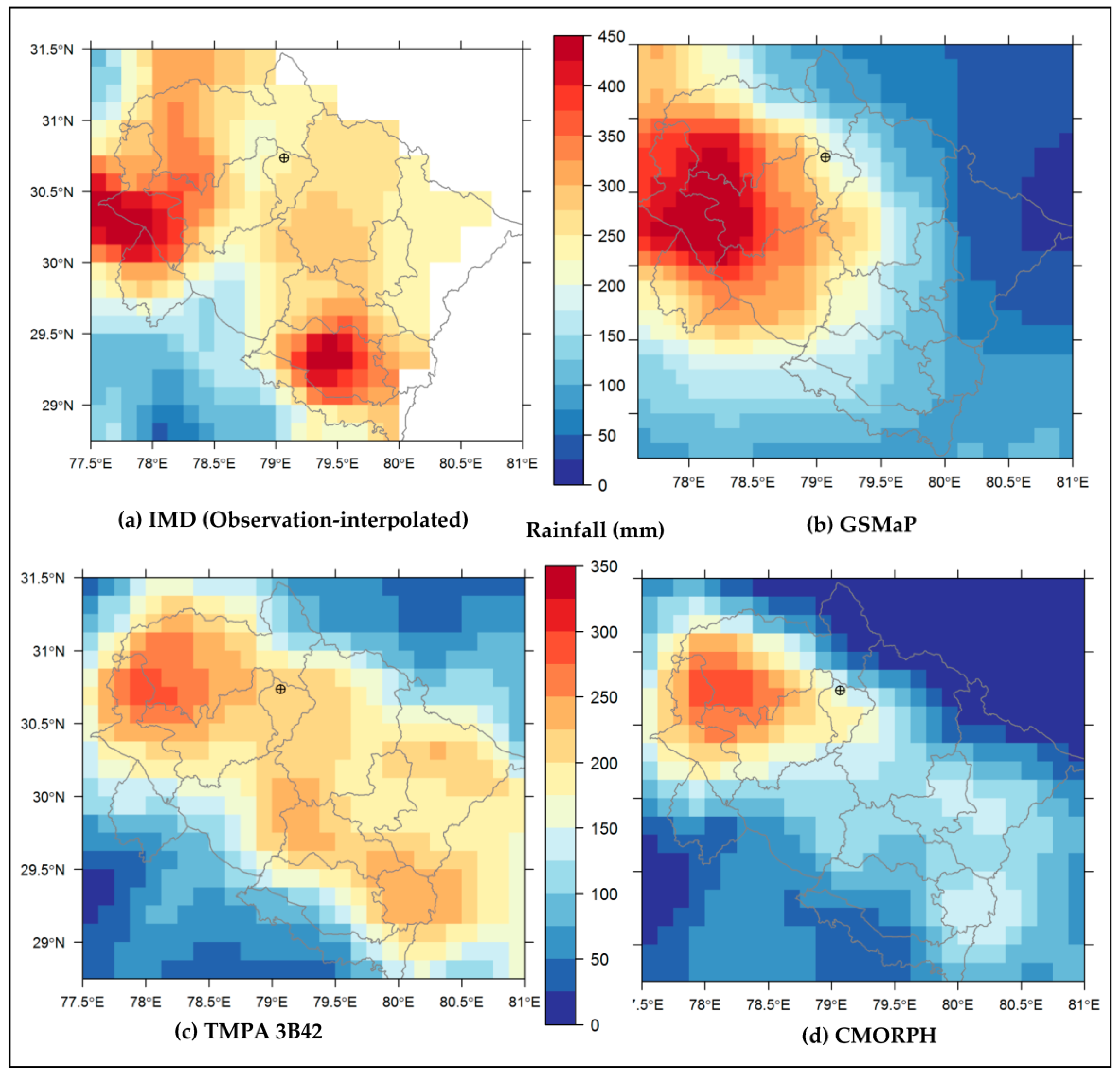
4.1. Spatial Pattern of Precipitation Retrieved from SBRE Products and Conventional IMD-Based Gauge Stations
4.2. SBRE Rainfall Products Validation against IMD Using Statistical Metrics
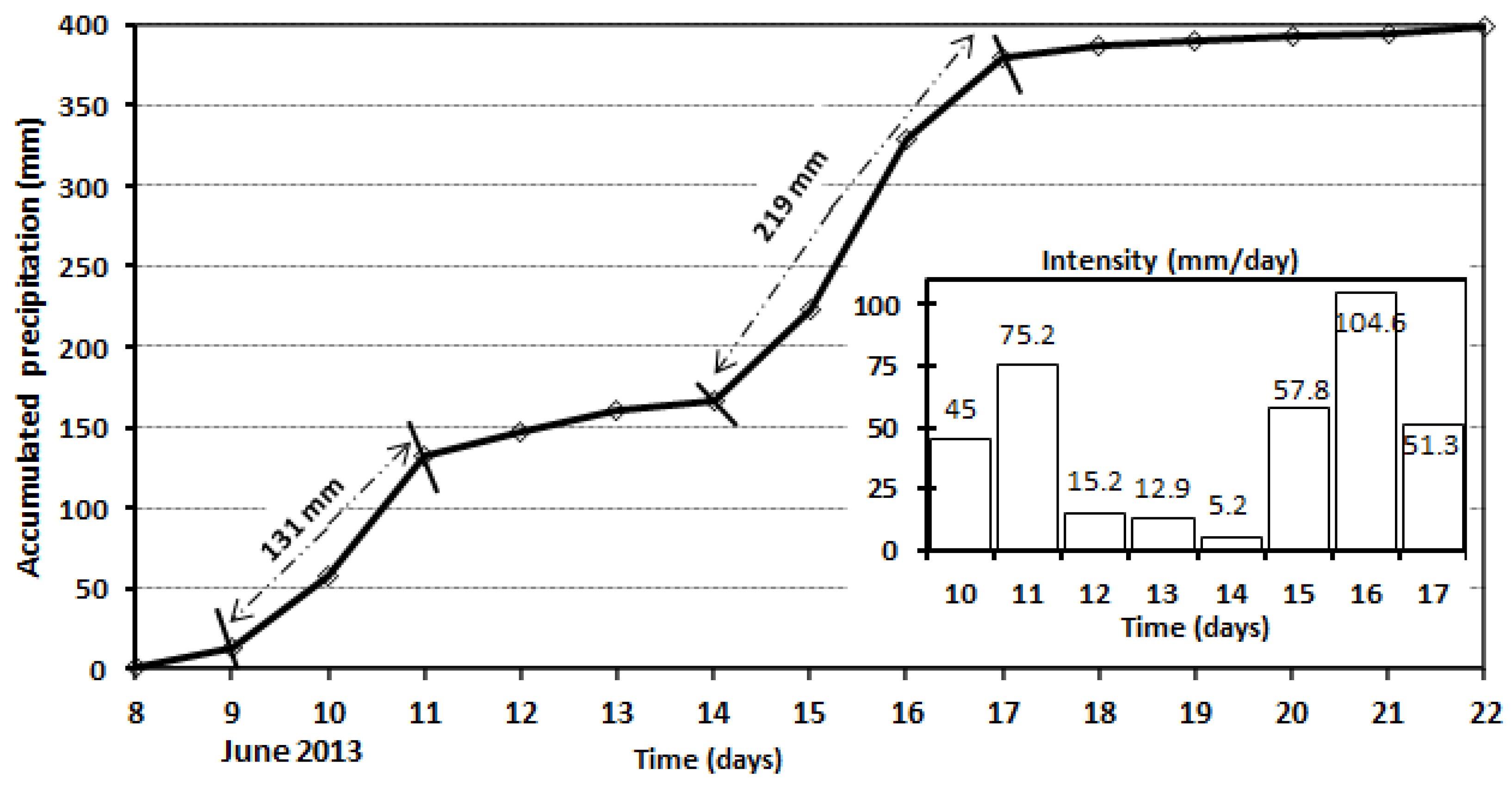
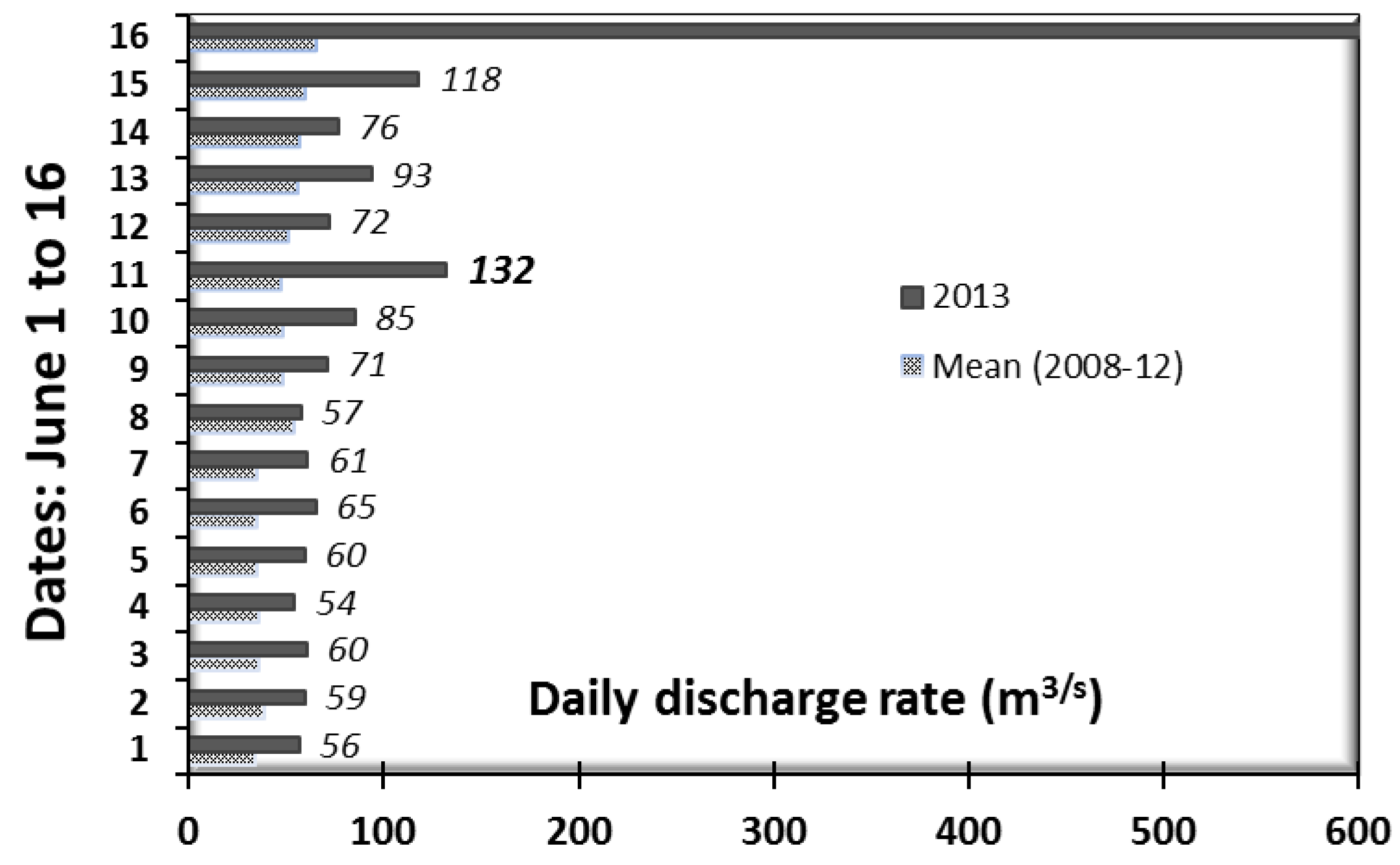
4.3. Observed Discharge Rate at Sitapur (Gaurikund) during 1–16 June 2013
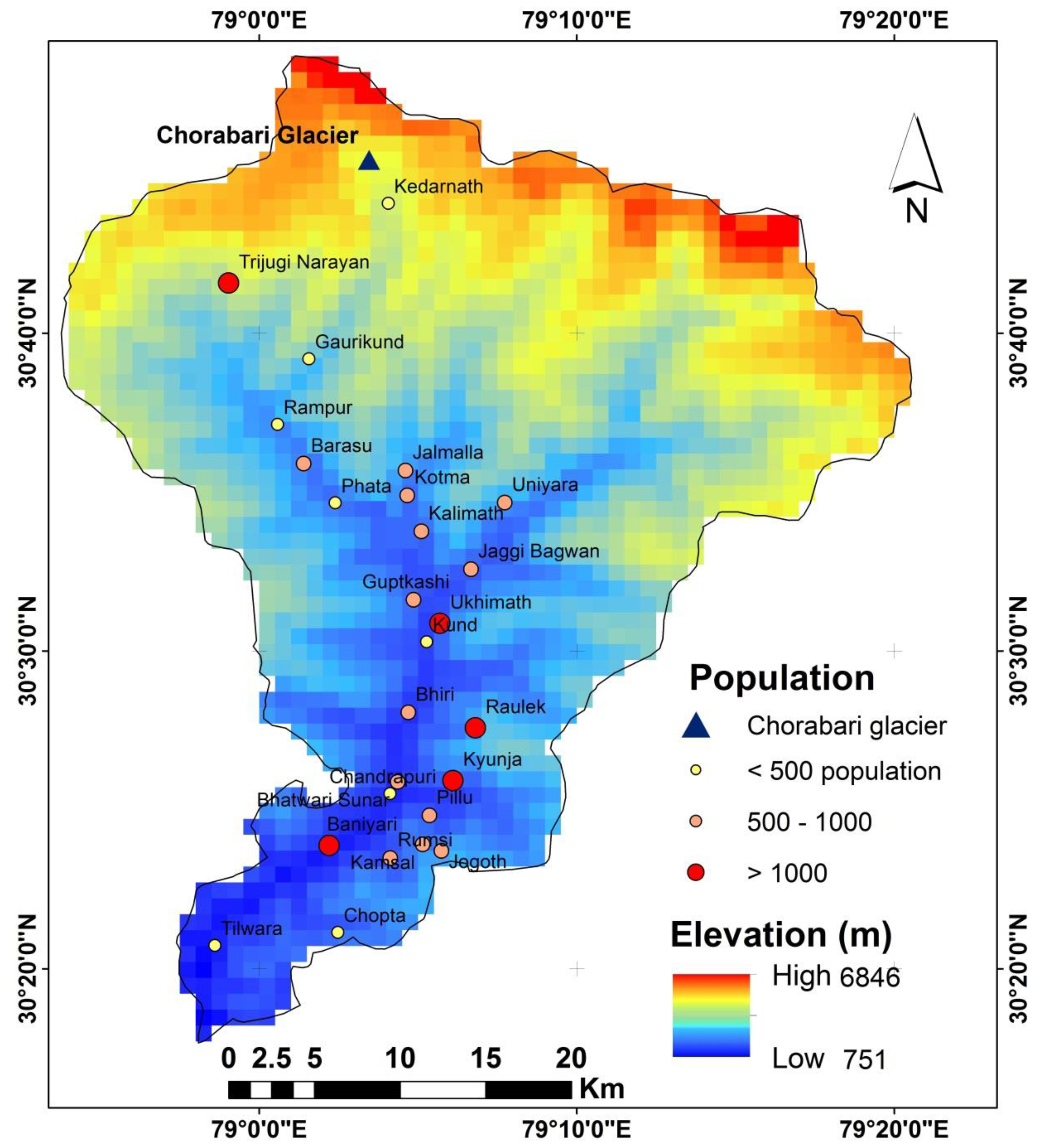
4.4. GIS-Based Mapping of Affected Villages and Population
5. Discussions and Conclusions
Acknowledgments
Author Contributions
Conflicts of Interest
Acronyms
| SBRE | Satellite Based Rainfall Estimates |
| TRMM | Tropical Rainfall Measuring Mission |
| TMPA | TRMM Multisatellite Precipitation Analysis |
| GSMaP | Global Satellite Mapping of Precipitation |
| CMORPH | Climate Prediction Center Morphing method |
| GCPC-1DD | Global Precipitation Climatology Project One Degree Daily estimate |
| APHRODITE | Asian Precipitation-Highly-Resolved Observational Data Integration towards Evaluation of Water Resources |
| RFE2 | African Rainfall Estimate |
| IMD | India Meteorological Department |
| NCC | National Climate Centre |
| NDC | National Data Center |
| WIHG | Wadia Institute of Himalayan Geology |
| PMW | Passive Microwave Radiometer |
| NOAA | National Oceanic and Atmospheric Administration |
| CPC | Climate Prediction Center |
| MAE | Mean Absolute Error |
| NRMSE | Normalized root mean square error |
| PBIAS | Percent Bias |
| NSE | Nash-Sutcliffe efficiency |
References
- Kotal, S.D.; Roy, S.S.; Bhowmik, S.K.R. Catastrophic heavy rainfall episode over Uttarakhand during 16–18 June 2013—Observational aspects. Curr. Sci. 2014, 107, 234–245. [Google Scholar]
- Das, S.; Ashrit, R.; Moncrieff, M.W. Simulation of a Himalayan cloudburst event. J. Earth Syst. Sci. 2006, 115, 299–313. [Google Scholar] [CrossRef]
- Rautela, P. Lessons learnt from the Deluge of Kedarnath, Uttarakhand, India. Asian J. Environ. Disaster Manag. 2013, 5, 43–51. [Google Scholar] [CrossRef]
- Dani, S.; Motwani, A. India-Uttarakand Disaster: Joint Rapid Damage and Needs Assessment Report 2013; World Bank: Washington, DC, USA, 2013. [Google Scholar]
- ICIMOD. Glacial Lakes and Glacial Lake Outburst Floods in Nepal; International Centre for Integrated Mountain Development (ICIMOD): Kathmandu, Nepal, 2011. [Google Scholar]
- Bookhagen, B.; Burbank, D.W. Toward a complete Himalayan hydrological budget: Spatiotemporal distribution of snowmelt and rainfall and their impact on river discharge. J. Geophys. Res. 2010, 115. [Google Scholar] [CrossRef]
- Bharti, V.; Singh, C. Evaluation of error in TRMM 3B42V7 precipitation estimates over the Himalayan region: EVALUATION OF ERROR IN TRMM 3B42V. J. Geophys. Res. Atmos. 2015, 120, 12458–12473. [Google Scholar] [CrossRef]
- Prakash, S.; Mitra, A.K.; Rajagopal, E.N.; Pai, D.S. Assessment of TRMM-based TMPA-3B42 and GSMaP precipitation products over India for the peak southwest monsoon season: ASSESSMENT OF TMPA AND GSMAP PRECIPITATION PRODUCTS OVER INDIA. Int. J. Climatol. 2016, 36, 1614–1631. [Google Scholar] [CrossRef]
- Chandra, M.; Kumar, R.; Kannan, B.A.M.; Reddy, Y.K.; Sastry, P.S. Standard Operating Procedure for Doppler Weather Radar-98d/s; Weather Radar Division, India Meteorol. Dep. Minist. Earth Sci., Gov. India: New Delhi, India, 2011.
- Huffman, G.J. Estimates of Root-Mean-Square Random Error for Finite Samples of Estimated Precipitation. J. Appl. Meteorol. 1997, 36, 1191–1201. [Google Scholar] [CrossRef]
- Huffman, G.J.; Bolvin, D.T.; Nelkin, E.J.; Wolff, D.B.; Adler, R.F.; Gu, G.; Hong, Y.; Bowman, K.P.; Stocker, E.F. The TRMM Multisatellite Precipitation Analysis (TMPA): Quasi-Global, Multiyear, Combined-Sensor Precipitation Estimates at Fine Scales. J. Hydrometeorol. 2007, 8, 38–55. [Google Scholar] [CrossRef]
- Gosset, M.; Viarre, J.; Quantin, G.; Alcoba, M. Evaluation of several rainfall products used for hydrological applications over West Africa using two high-resolution gauge networks. Q. J. R. Meteorol. Soc. 2013, 139, 923–940. [Google Scholar] [CrossRef]
- Hamada, A.; Murayama, Y.; Takayabu, Y.N. Regional Characteristics of Extreme Rainfall Extracted from TRMM PR Measurements. J. Clim. 2014, 27, 8151–8169. [Google Scholar] [CrossRef]
- Zhao, H.; Yang, S.; Wang, Z.; Zhou, X.; Luo, Y.; Wu, L. Evaluating the suitability of TRMM satellite rainfall data for hydrological simulation using a distributed hydrological model in the Weihe River catchment in China. J. Geogr. Sci. 2015, 25, 177–195. [Google Scholar] [CrossRef]
- Parida, B.R.; Collado, W.B.; Borah, R.; Hazarika, M.K.; Samarakoon, L. Detecting Drought-Prone Areas of Rice Agriculture Using a MODIS-Derived Soil Moisture Index. GIScience Remote Sens. 2008, 45, 109–129. [Google Scholar] [CrossRef]
- Li, Z.; Yang, D.; Hong, Y. Multi-scale evaluation of high-resolution multi-sensor blended global precipitation products over the Yangtze River. J. Hydrol. 2013, 500, 157–169. [Google Scholar] [CrossRef]
- Li, Z.; Yang, D.; Gao, B.; Jiao, Y.; Hong, Y.; Xu, T. Multiscale Hydrologic Applications of the Latest Satellite Precipitation Products in the Yangtze River Basin using a Distributed Hydrologic Model. J. Hydrometeorol. 2015, 16, 407–426. [Google Scholar] [CrossRef]
- Krajewski, W. Ground networks: Are we doing the right things? In Measuring Precipitation from Space—EURAINSAT and the Future; Levizzani, V., Bauer, P., Turk, F.J., Eds.; Springer: Dordrecht, The Netherlands, 2007; Volume 28, pp. 403–417. [Google Scholar]
- Dinku, T.; Chidzambwa, S.; Ceccato, P.; Connor, S.J.; Ropelewski, C.F. Validation of high-resolution satellite rainfall products over complex terrain. Int. J. Remote Sens. 2008, 29, 4097–4110. [Google Scholar] [CrossRef]
- Gebregiorgis, A.S.; Hossain, F. How well can we estimate error variance of satellite precipitation data around the world? Atmos. Res. 2015, 154, 39–59. [Google Scholar] [CrossRef]
- Artan, G.; Gadain, H.; Smith, J.L.; Asante, K.; Bandaragoda, C.J.; Verdin, J.P. Adequacy of satellite derived rainfall data for stream flow modeling. Nat. Hazards 2007, 43, 167–185. [Google Scholar] [CrossRef]
- Bookhagen, B.; Burbank, D.W. Topography, relief, and TRMM-derived rainfall variations along the Himalaya. Geophys. Res. Lett. 2006, 33. [Google Scholar] [CrossRef]
- McCollum, J.R.; Gruber, A.; Ba, M.B. Discrepancy between Gauges and Satellite Estimates of Rainfall in Equatorial Africa. J. Appl. Meteorol. 2000, 39, 666–679. [Google Scholar] [CrossRef]
- Gupta, A.K.; Dobhal, D.P.; Mehta, M.; Verma, A.; Pratap, B.; Kesarwani, K. A Report on Kedarnath Devastation; Wadia Institute of Himalayan Geology: Dehradun, Uttrakhand, India, 2013; pp. 1–64. [Google Scholar]
- Mehta, M.; Dobhal, D.P.; Kesarwani, K.; Pratap, B.; Kumar, A.; Verma, A. Monitoring of Glacier Changes and Response Time in Chorabari Glacier, Central Himalaya, Garhwal, India. Curr. Sci. 2014, 107, 281–289. [Google Scholar]
- DMMC Report. Geological Investigations in Rudraprayag District with Special Reference to Mass Instability; Disaster Mitigation and Management Centre, Gov. of Uttarakhand: Uttarakhand, India, 2014.
- Huffman, G.J.; Adler, R.F.; Bolvin, D.T.; Nelkin, E.J. The TRMM Multi-Satellite Precipitation Analysis (TMPA). In Satellite Rainfall Applications for Surface Hydrology; Gebremichael, M., Hossain, F., Eds.; Springer: Dordrecht, The Netherlands, 2010; pp. 3–22. [Google Scholar]
- Huffman, G.J.; Bolvin, D.T. TRMM and Other Data Precipitation Data Set Documentation 2013. Available online: ftp://meso-a.gsfc.nasa.gov/pub/trmmdocs/3B42_3B43_doc.pdf (accessed on 5 July 2016).
- Shepard, D. A Two-dimensional Interpolation Function for Irregularly-spaced Data. In Proceedings of the 1968 23rd ACM National Conference, Las Vegas, NV, USA, 27–29 August 1968; ACM: New York, NY, USA, 1968; pp. 517–524. [Google Scholar]
- Pai, D.S.; Sridhar, L.; Rajeevan, M.; Sreejith, O.P.; Satbhai, N.S.; Mukhopadhyay, B. Development of a new high spatial resolution (0.25° × 0.25°) long period (1901–2010) daily gridded rainfall data set over India and its comparison with existing data sets over the region. Mausam 2014, 65, 1–18. [Google Scholar]
- Joyce, R.J.; Janowiak, J.E.; Arkin, P.A.; Xie, P. CMORPH: A Method that Produces Global Precipitation Estimates from Passive Microwave and Infrared Data at High Spatial and Temporal Resolution. J. Hydrometeorol. 2004, 5, 487–503. [Google Scholar] [CrossRef]
- Ushio, T.; Sasashige, K.; Kubota, T.; Shige, S.; Okamoto, K.; Aonashi, K.; Inoue, T.; Takahashi, N.; Iguchi, T.; Kachi, M.; et al. A Kalman Filter Approach to the Global Satellite Mapping of Precipitation (GSMaP) from Combined Passive Microwave and Infrared Radiometric Data. J. Meteorol. Soc. Jpn. Ser II 2009, 87A, 137–151. [Google Scholar] [CrossRef]
- Janowiak, J.E.; Kousky, V.E.; Joyce, R.J. Diurnal cycle of precipitation determined from the CMORPH high spatial and temporal resolution global precipitation analyses. J. Geophys. Res. 2005, 110. [Google Scholar] [CrossRef]
- Ushio, T.; Tashima, T.; Kubota, T.; Kachi, M. Gauge Adjusted Global Satellite Mapping of Precipitation (GSMaP_Gauge). In Proceedings of the 29th ISTS, Nagoya, Japan, 2–9 June 2013. [Google Scholar]
- Pai, D.S.; Sridhar, L.; Badwaik, M.R.; Rajeevan, M. Analysis of the daily rainfall events over India using a new long period (1901–2010) high resolution (0.25° × 0.25°) gridded rainfall data set. Clim. Dyn. 2015, 45, 755–776. [Google Scholar] [CrossRef]
- Rajeevan, M.; Bhate, J. A high resolution daily gridded rainfall dataset (1971–2005) for mesoscale meteorological studies. Curr. Sci. 2009, 96, 558–562. [Google Scholar]
- Krishnamurthy, V.; Shukla, J. Intraseasonal and Seasonally Persisting Patterns of Indian Monsoon Rainfall. J. Clim. 2007, 20, 3–20. [Google Scholar] [CrossRef]
- Krishnamurthy, V.; Shukla, J. Seasonal persistence and propagation of intraseasonal patterns over the Indian monsoon region. Clim. Dyn. 2008, 30, 353–369. [Google Scholar] [CrossRef]
- Srinivasan, J.; Joshi, P.C. What have we learned about the Indian monsoon from satellite data? Curr. Sci. 2007, 93, 165–172. [Google Scholar]
- Yatagai, A.; Kamiguchi, K.; Arakawa, O.; Hamada, A.; Yasutomi, N.; Kitoh, A. APHRODITE: Constructing a Long-Term Daily Gridded Precipitation Dataset for Asia Based on a Dense Network of Rain Gauges. Bull. Am. Meteorol. Soc. 2012, 93, 1401–1415. [Google Scholar] [CrossRef]
- Dobhal, D.P.; Gupta, A.K.; Mehta, M.; Khandelwal, D.D. Kedarnath disaster: Facts and plausible causes. Curr. Sci. 2013, 105, 171–174. [Google Scholar]
- Rudraprayag-Uttarakhand District Administration 2014. Available online: http://rudraprayag.nic.in (accessed on 5 August 2016).
- Census India. 2011. Available online: http://census2011.co.in (accessed on 5 June 2016).
- Devastating Flash Floods in Uttarakhand and Himachal Pradesh 2013, Pragya. Available online: www.pragya.org/doc/flashflood_update.pdf (accessed on 5 February 2015).
- Report for Relief Work Uttarakhand Disaster 2013 by Partners of Association for India’s Development, AID-JHU. Available online: www.aidjhu.org (accessed on 5 May 2016).
- Global 30 Arc-Second Elevation (GTOPO30)|The Long Term Archive. Available online: https://lta.cr.usgs.gov/GTOPO30 (accessed on 8 May 2016).
- Uttarakhand Tourism Development Board (UTDB). Available online: http://uttarakhandtourism.gov.in (accessed on 20 October 2016).
- Hijmans, R.J.; van Etten, J.; Cheng, J.; Mattiuzzi, M.; Sumner, M.; Greenberg, J.A.; Lamigueiro, O.P.; Bevan, A.; Racine, E.B.; Shortridge, A.; et al. Geographic Data Analysis and Modeling [R package Raster Version 2.5-2]. Available online: https://CRAN.R-project.org/package=raster (accessed on 15 February 2016).
- Pebesma, E.; Bivand, R.; Rowlingson, B.; Gomez-Rubio, V.; Hijmans, R.; Sumner, M.; MacQueen, D.; Lemon, J.; O’Brien, J. Classes and Methods for Spatial Data [R package sp version 1.2-1]. Available online: https://CRAN.R-project.org/package=sp (accessed on 5 March 2016).
- Nash, J.E.; Sutcliffe, J.V. River flow forecasting through conceptual models part I—A discussion of principles. J. Hydrol. 1970, 10, 282–290. [Google Scholar] [CrossRef]
- Legates, D.R.; McCabe, G.J. Evaluating the use of “goodness-of-fit” Measures in hydrologic and hydroclimatic model validation. Water Resour. Res. 1999, 35, 233–241. [Google Scholar] [CrossRef]
- Durga Rao, K.H.V.; Rao, V.V.; Dadhwal, V.K.; Diwakar, P.G. Kedarnath flash floods: A hydrological and hydraulic simulation study. Curr. Sci. 2014, 106, 598–603. [Google Scholar]
- Chopra, R. Uttarakhand: Development and Ecological Sustainability; Oxfam: New Delhi, India, 2014. [Google Scholar]
- Hong, Y.; Adler, R.F.; Negri, A.; Huffman, G.J. Flood and landslide applications of near real-time satellite rainfall products. Nat. Hazards 2007, 43, 285–294. [Google Scholar] [CrossRef]
- Shrestha, M.S.; Artan, G.A.; Bajracharya, S.R.; Sharma, R.R. Using satellite-based rainfall estimates for streamflow modelling: Bagmati Basin: Rainfall estimates for streamflow modelling. J. Flood Risk Manag. 2008, 1, 89–99. [Google Scholar] [CrossRef]
- Mishra, A.; Srinivasan, J. Did a cloud burst occur in Kedarnath during 16 and 17 June 2013? Curr. Sci. 2013, 105, 1351–1352. [Google Scholar]
- Bharti, V.; Singh, C.; Ettema, J.; Turkington, T.A.R. Spatiotemporal characteristics of extreme rainfall events over the Northwest Himalaya using satellite data: SPATIOTEMPORAL CHARACTERISTICS OF EXTREME RAINFALL EVENTS. Int. J. Climatol. 2016, 36, 3949–3962. [Google Scholar] [CrossRef]
- Dinku, T.; Connor, S.J.; Ceccato, P. Comparison of CMORPH and TRMM-3B42 over Mountainous Regions of Africa and South America. In Satellite Rainfall Applications for Surface Hydrology; Gebremichael, M., Hossain, F., Eds.; Springer: Dordrecht, The Netherlands, 2010; pp. 193–204. [Google Scholar]
- NRSC and Bhuvan. Available online: http://bhuvan.nrsc.gov.in/updates/gallery (accessed on 18 February 2016).
- Allen, S.K.; Rastner, P.; Arora, M.; Huggel, C.; Stoffel, M. Lake outburst and debris flow disaster at Kedarnath, June 2013: Hydrometeorological triggering and topographic predisposition. Landslides 2016, 13, 1479–1491. [Google Scholar] [CrossRef]
- Singh, D.; Horton, D.; Tsiang, M.; Haugen, M.; Ashfaq, M.; Mei, R.; Rastogi, D.; Johnson, N.; Charland, A.; Rajaratnam, B.; et al. Severe precipitation in northern India in June 2013: Causes, historical context, and changes in probability. Bull. Am. Meteorol. Soc. 2014, 95, S58–S61. [Google Scholar]
- Siderius, C.; Biemans, H.; Wiltshire, A.; Rao, S.; Franssen, W.H.P.; Kumar, P.; Gosain, A.K.; van Vliet, M.T.H.; Collins, D.N. Snowmelt contributions to discharge of the Ganges. Sci. Total Environ. 2013, 468–469, S93–S101. [Google Scholar] [CrossRef] [PubMed]
- NIDM, Uttarakhand. National Disaster Risk Reduction Portal; Ministry of Home Affairs, Gov. of India: New Delhi, India, 2014; pp. 1–20.
- Semwal, R.; Kumar, K.; Dhyani, P.P. Regulating tourism and pilgrimage in the Himalaya. Curr. Sci. 2014, 106, 797. [Google Scholar]


| Features | Conventional Data | SBRE Products | ||
|---|---|---|---|---|
| IMD-Gauge | TMPA-3B42 (v7) | CMORPH | GSMaP | |
| Spatial & Temporal resolution | 0.25° grid | 0.25° grid | 0.25° grid | 0.1° grid |
| Daily | Daily | 3-hourly | Daily | |
| Sensors involved | - | IR, TMI, SSM/I, AMSR-E, AMSU-B, MHS | IR, TMI, SSM/I, AMSR-E, AMSU-B | IR, TMI, SSM/I, AMSR-E, AMSU-B |
| Interpolation method | IDW [29] | - | - | - |
| Coverage | India | Global | Global | Global |
| Gauge calibrated | Yes | Yes | No | Yes |
| Agency | IMD | NASA & JAXA | NOAA CPC | JAXA |
| Reference | [30] | [10] | [31] | [32] |
| Parameters | TMPA-3B42 (v7) | GSMaP | CMORPH |
|---|---|---|---|
| PBIAS (%) | −18.2 | 14.4 | −29.0 |
| MAE (mm) | 52.7 | 71.8 | 82.5 |
| NRMSE (%) | 21.5 | 28.0 | 33.0 |
| NSE | −0.93 | −2.25 | −3.52 |
| Rain-Gauge Stations | Accumulated Rainfall | Maximum Intensity (mm/Day) | Maximum Intensity (Date) |
|---|---|---|---|
| (IMD gauge-based point observations) | |||
| Uttarkashi | 359 | 162 | 17 June |
| Jakoli, Rudraprayag | 390 | 121 | 16 June |
| Tharali, Chamoli | 326 | 173 | 17 June |
| Pithoragarh | 214 | 117.2 | 18 June |
| (WIHG observatory near Kedarnath) | |||
| Kopardhar, Ghuttu | 275 | 122 | 16 June |
| (TMPA-3B42 (area averaged over Kedarnath, Figure 4) | |||
| Kedarnath | 227.5 | 105 | 16 June |
| Years | Kedarnath | Badrinath |
|---|---|---|
| 1990 | 0.117 | 0.362 |
| 2000 | 0.215 | 0.735 |
| 2005 | 0.390 | 0.566 |
| 2010 | 0.400 | 0.921 |
| 2012 | 0.548 | 0.986 |
| 2013 | 0.312 | 0.497 |
| 2014 | 0.048 | 0.180 |
| 2015 | 0.154 | 0.359 |
© 2017 by the authors. Licensee MDPI, Basel, Switzerland. This article is an open access article distributed under the terms and conditions of the Creative Commons Attribution (CC BY) license (http://creativecommons.org/licenses/by/4.0/).
Share and Cite
Parida, B.R.; Behera, S.N.; Bakimchandra, O.; Pandey, A.C.; Singh, N. Evaluation of Satellite-Derived Rainfall Estimates for an Extreme Rainfall Event over Uttarakhand, Western Himalayas. Hydrology 2017, 4, 22. https://doi.org/10.3390/hydrology4020022
Parida BR, Behera SN, Bakimchandra O, Pandey AC, Singh N. Evaluation of Satellite-Derived Rainfall Estimates for an Extreme Rainfall Event over Uttarakhand, Western Himalayas. Hydrology. 2017; 4(2):22. https://doi.org/10.3390/hydrology4020022
Chicago/Turabian StyleParida, Bikash Ranjan, Sailesh N. Behera, Oinam Bakimchandra, Arvind Chandra Pandey, and Nilendu Singh. 2017. "Evaluation of Satellite-Derived Rainfall Estimates for an Extreme Rainfall Event over Uttarakhand, Western Himalayas" Hydrology 4, no. 2: 22. https://doi.org/10.3390/hydrology4020022