
Understanding the Effects of Parameter Uncertainty on Temporal Dynamics of Groundwater-Surface Water Interaction

1
Institute for Environmental Sustainability, Mount Royal University, Calgary, AB. T3E 6k6, Canada
2
Environmental Engineering Program, University of Northern British Columbia, Prince George, B.C. V2N 4Z9, Canada
*
Author to whom correspondence should be addressed.
Hydrology 2017, 4(2), 28; https://doi.org/10.3390/hydrology4020028
Submission received: 29 March 2017
/
Revised: 6 May 2017
/
Accepted: 8 May 2017
/
Published: 12 May 2017
(This article belongs to the Special Issue Groundwater Flow)
Abstract
:This study presents the understanding of temporal dynamics of groundwater-surface water (GW-SW) interaction due to parameter uncertainty by using a physically-based and distributed gridded surface subsurface hydrologic analysis (GSSHA) model combined with a Monte Carlo simulation. A study area along the main stem of the Kiskatinaw River of the Kiskatinaw River watershed, Northeast British Columbia, Canada, was used as a case study. Two different greenhouse gas (GHG) emission scenarios (i.e., A2: heterogeneous world with self-reliance and preservation of local identities, and B1: a more integrated and environmental-friendly world) of the Special Report on Emissions Scenarios (SRES) from the Fourth Assessment Report of the Intergovernmental Panel on Climate Change (IPCC) for 2013 were used as case scenarios. Before conducting uncertainty analysis, a sensitivity analysis was performed to find the most sensitive parameters to the model output (i.e., mean monthly groundwater contribution to stream flow). Then, a Monte Carlo simulation was used to conduct the uncertainty analysis. The uncertainty analysis results under both case scenarios revealed that the pattern of the cumulative relative frequency distribution of the mean monthly and annual groundwater contributions to stream flow varied monthly and annually, respectively, due to the uncertainties of the sensitive model parameters. In addition, the pattern of the cumulative relative frequency distribution of a particular month’s groundwater contribution to the stream flow differed significantly between both scenarios. These results indicated the complexities and uncertainties in the GW-SW interaction system. Therefore, it is of necessity to use such uncertainty analysis results rather than the point estimates for better water resources management decision-making.
1. Introduction
Groundwater-surface water (GW-SW) interaction plays a vital role in the functioning of riparian ecosystems [1]. During wet periods, surface water can recharge groundwater, but during dry periods groundwater can act as an important source to feed the surface water flow. As a result, groundwater and surface water are closely-linked components of the hydrologic system due to their interdependency to each other. The development and exploitation of any one component can affect the other. Therefore, for developing sustainable water resources management, it is crucial to understand and quantify the exchange processes between these two components [2]. During the last decade, many researchers have used different hydrologic models to quantify these exchange processes. For instance, Scibek and Allen [3] used the coupled Hydrologic Evaluation of Landfill Performance (HELP) and visual MODular three-dimensional finite-difference groundwater FLOW (MODFLOW) model; Van Roosmalen et al. [4] used the DK model (The National Water Resource model for Denmark); Goderniaux et al. [5] used the HydroGeoSphere model; Stoll et al. [6] used the MIKE Système Hydrologique Européen (MIKE-SHE) model; Jackson et al. [7] used the coupled Zoom Object-Oriented Distributed Recharge Model (ZOODRM) and Zoom Object-Oriented Quasi-3-Dimensional Model (ZOOMQ3D); Vansteenkiste et al. [8] used the MIKE-SHE, and Water and Energy Transfer between Soil, Plants and Atmosphere (WetSpa) models; El Hassan et al. [9] used the Gridded Surface Subsurface Hydrologic Analysis (GSSHA) model; Wu et al. [10] used Groundwater and Surface-water FLOW (GSFLOW) model; Faramarzi et al. [11] used the Soil and Water Assessment Tool (SWAT) model. Most of the parameters (e.g., soil properties, surface roughness) in hydrologic models used for GW-SW interaction simulations require intensive field measurements [12], and they are always associated with uncertainty. Such uncertainty could also lead to uncertainty in modeling outputs [13], which could jeopardize the decision-making of water resources management. The uncertainty analysis could provide a range of outputs instead of one output, and enable the watershed manager to take proper action with respect to water withdrawal from the river, and allocation to the stakeholders for future water supply depending on the month and season.
Due to the importance of parameter uncertainty in hydrologic models, many researchers used different uncertainty analysis methods in different hydrologic models to conduct uncertainty analysis of modeling outputs during the last several decades. For example, Beven and Binley [14] used the Generalized Likelihood Uncertainty Estimation (GLUE) method in the Institute of Hydrology Distributed Model (IHDM) to investigate how the stream flow hydrograph varies under the parameter uncertainty during a number of storms in the Gwy catchment, Wales. Kuczera and Mroczkowski [15] assessed the use of multinormal approximation to parameter uncertainty for the exploration of multiresponse data (i.e., stream flow, stream chloride concentration, groundwater level) in the CATPRO hydrosalinity model in the Wights catchment in Western Australia. Vrugt et al. [16] used the Markov Chain Monte Carlo (MCMC) method in the HYdrological MODel (HYMOD) to find out the variation of stream flow under the parameter uncertainty in the Leaf River watershed, Mississippi, USA. Benke et al. [12] used the Monte Carlo simulation (MCS) method as an uncertainty analysis method in the 2C hydrological model to investigate the impacts of parameter uncertainty on the prediction of stream flow in Eastern Australia. Mishra [17] used the first-order second-moment (FOSM) and MCS methods in the Natural Systems Regional Simulation Model (NSRSM) to compare the impacts of parameter uncertainty on stream flow prediction in Southern Florida, USA. Shen et al. [18,19] used GLUE and MCS methods, respectively, in the SWAT model to quantify the effects of parameter uncertainty on stream flow and sediment in the Daning River watershed of the Three Gorges Reservoir Region, China. Wu et al. [10] used the Probabilistic Collocation Method (PCM) in the GSFLOW model for integrated modeling of GW-SW systems (i.e., annual stream flow, annual GW-SW exchange, and annual groundwater level) in the Heihe River Basin, China. Fan et al. [20] used PCM and MCS methods in the HYMOD to compare the uncertainty of stream flow predictions due to the parameter uncertainty in the Xiangxi River basin of the Three Gorges Reservoir Region, China. Fan et al. [21] used the Hybrid Sequential Data Assimilation and Probabilistic Collocation (HSDAPC) method in the HYMOD for analyzing uncertainty of stream flow predictions due to the parameter uncertainty in the Xiangxi River basin of the Three Gorges Reservoir Region, China. Wu et al. [22] used CoupModel combined with the GLUE method to investigate the water and energy balance in seasonally-frozen soils due to parameter uncertainty in Northern China. Faramarzi et al. [11] used multivariate uniform distribution in the SWAT model to assess uncertainty of freshwater scarcity in semi-arid watersheds of Alberta, Canada. However, there is little knowledge regarding the uncertainty analysis of mean monthly (i.e., intra-annual) and annual groundwater contributions to stream flow due to parameter uncertainty in a watershed. The objective of the study was to understand and find out the variation of the mean monthly and annual groundwater contributions to stream flow due to parameter uncertainty. These contributions information will be useful in determining the temporal status of groundwater resources and site conditions for groundwater-dependent terrestrial ecosystems [23]. They will also determine the temporal variations of stream flow dependency on groundwater, and these will provide useful information for both short and long-term water withdrawal from the river and water supply decision-making. This study also presents a new technique to understand temporal dynamics of GW-SW interaction systems by using temporal mean groundwater contributions to the stream flow. A GSSHA hydrologic model was developed for this study in a study area along the main stem of the Kiskatinaw River of the Kiskatinaw River watershed (KRW) in Northeastern British Columbia, Canada. The A2 and B1 greenhouse gas (GHG) emission scenarios of SRES (Special Report on Emissions Scenarios) of the Intergovernmental Panel on Climate Change (IPCC) of 2013 were used as case scenarios. Before conducting uncertainty analysis, a sensitivity analysis was conducted to find out the most sensitive parameters to the model outputs. Then Monte Carlo realizations of the most sensitive modeling parameters were generated for the GSSHA model to conduct the uncertainty analysis of the temporal dynamics of the GW-SW interaction.
2. Study Area
The Kiskatinaw River watershed (KRW) is a multi-use watershed located in Northeast British Columbia, Canada, as shown in Figure 1. The KRW provides water for drinking water supply and household activities, timber harvesting, oil and gas, agriculture, wildlife, recreation, and mineral resources. The City of Dawson Creek has been using water from Kiskatinaw River for drinking purpose since the mid-1940s because of the presence of high total hardness in groundwater of this region [24]. The water demand in the KRW increased significantly after 2005 because of shale gas exploration/production activities. The large scale of shale gas exploration/production, timber harvesting, and agricultural activities in recent years have resulted in water conflicts among various water users.
The study area (213.82 km2) is situated along the main stem of the Kiskatinaw River in the KRW (Figure 1). The City of Dawson Creek’s drinking water intake of the water supply system is located at Arras in the study area. The elevation of the study area ranges from 687 m to 950 m, and the mean slope is 7.8% [25]. The dominant soil texture in the study area is mainly clay loam (91%), although silt loam and sandy loam occupy 6% and 3% of the study area, respectively. The study area is mainly a forested area (68%) (Figure 1). Other land use types are forest clear cut (18.7%), agriculture (8%), wetland (2%), water (1.8%), and built up area (1.5%).
The hydrologic system in the KRW is flashy, with peak flows occurring from late June to early July, but in January the flow drops to 0.052 m3/s [24]. The mean annual precipitation and temperature in the KRW is 499 mm, and 2.7 °C, respectively (mean over the period of 2000–2011). The major portion of the precipitation is rainfall (320 mm), therefore, the hydrologic system in the KRW is rain dominated. Previous studies reported that the river system in the KRW is groundwater dependent [25,26]. Therefore, it is very important to conduct an uncertainty analysis of GW-SW interaction in the study area to understand those interactions and develop future water resources management plans.
3. Materials and Methods
3.1. GW-SW Interaction Modeling
In order to conduct an uncertainty analysis of GW-SW interaction, a physically-based, distributed and structured grid-based GSSHA hydrologic model was developed for the study area. The model domain was discretized into grid cells of 30 m by 30 m. In GSSHA model, infiltration was computed by using the Green and Ampt infiltration with a redistribution method [27]. Saturated groundwater flow was computed by using a finite difference representation of the following 2-D lateral saturated groundwater flow equation:
where Kx is the hydraulic conductivity of soil in x direction, Ky is the hydraulic conductivity of soil in y direction, h is the hydraulic head, S is the storage term, b is the depth of the saturated media, and W is the flux term for sources and sinks. Water flux between the stream and the saturated groundwater was estimated by using Darcy’s law and the following equation:
where f is the flux between the stream and the saturated groundwater, Ksb is the hydraulic conductivity of the streambed material, Msb is the depth of the streambed material, Egw is the elevation of groundwater surface, and Esb is the elevation of stream water surface. Groundwater discharge was then calculated by multiplying this f by the top width and length of the channel segment. Overland flow was simulated by using the Alternating Direction Explicit (ADE) finite difference method, while channel flow was simulated by using an explicit solution of the diffusive wave equation. The details of GSSHA can be found from Downer [28].
The GSSHA model requires a number of inputs, such as watershed specific data (i.e., elevation, channel geometry, soil type, and land use/land cover), hydrological (i.e., stream flow, and groundwater level) data, and climate (i.e., precipitation and temperature) and meteorological (i.e., wind speed, relative humidity, barometric pressure, direct and global radiations) data. The details of these data for this study were listed in Table 1. In this study, width and length of the channel segment were assumed constant. Observed hourly climate and meteorological data of three nearby weather stations were averaged by an arithmetic method to obtain daily distribution of those parameters for 2000–2011. In addition, in this study the soils of the study area were assumed as isotropic because the stratification of the soil layers of the study area were not available. Since GSSHA is a grid-based model, three index maps were prepared for assigning parameters at the grid level. One is a land use index map, and others are a soil type index map and a combined land use and soil type index map. In addition, initial groundwater table and aquifer (unconfined) bottom maps were prepared by using the inverse distance weighted (IDW) interpolation method. The distance between ground elevation and aquifer bottom elevation was used to make the vertical layer of the modeling domain. A similar approach was used by Woldeamlak et al. [32] in their developed model for investigating GW-SW interaction. The barometric pressure correction was estimated as per the technical guidelines of Solinst [33] to correct the groundwater table data because groundwater table fluctuates by atmospheric pressure with altitude change [34]. Around the perimeter of the study area, no-flow boundary condition was chosen for the developed model based on previous studies results [35]. In addition, the flux river boundary condition was chosen for the stream because of the significant exchange between groundwater and the stream network. Then the model was calibrated using Shuffled Complex Evolution method (automated calibration). Due to the limited observed stream flow data, the model calibration was conducted for the time period from 15 October 2010 to 31 December 2011. A simulation time step of 1 min was used for calibration and validation based on the temporal convergence study of observed and simulated stream flows at the outlet of the study area. There was flood in the KRW in 2011, and the model calibration was conducted to evaluate the performance of the model during flooding year. During calibration (Figure 2a), R2 (coefficient of determination) = 0.67, and NSE (Nash-Sutcliffe efficiency) = 0.62 were obtained. Santhi et al. [36] and Van Liew et al. [37] suggested an acceptable model evaluation when R2 value of greater than 0.5 obtained. These evaluation statistics criteria indicated satisfactory GSSHA model calibration. The calibrated parameters were tabulated in Table 2. Model validation was performed for the time period from 15 October 2006 to 15 October 2010, and this time period was normal annual precipitation years. The modeling validation results (Figure 2b) presented R2 = 0.63, and NSE = 0.58. Therefore, satisfactory model validation was also achieved. During calibration and validation periods, the flow direction was from groundwater to surface water, which indicates gaining stream or groundwater discharging to the stream.
3.2. Generation of Case Scenarios
Two case scenarios were generated to understand and find out the variation of the mean monthly and annual groundwater contributions to stream flow due to parameter uncertainty. Those scenarios were generated by using two climate change scenarios for 2013, which were obtained from CRCM 4.2 (Canadian Regional Climate Model) modeling outputs of the CCCma (Canadian Centre for Climate Modeling and Analysis). Those scenarios were A2 and B1 GHG emission scenarios of SRES of the IPCC [38]. The A2 scenario was used because it corresponds to regional economic development, and the large-scale shale gas exploration/production activities began in the KRW during 2005, and enhanced regional economy [39]. The B1 scenario was selected because it represents a more integrated and environmental friendly world [38]. These CRCM outputs are monthly means for two GHG emission scenarios [40]. For each scenario, three CRCM outputs were averaged as a mean. A similar approach was applied in various hydrological studies [3,8]. Then those outputs were distributed as daily values in the particular month by using the delta change method. This method is a commonly used simple downscaling method to deal with biases when using climate model outputs in hydrological studies at the catchment or sub-watershed scale [41,42]. This method has been used in a number of hydrological impact studies [4,40,43,44,45]. The details of delta change method can be found in Graham et al. [44], van Roosmalen et al. [4], and van Roosmalen et al. [45].
The temperature outputs from the delta change method showed that the trend of the mean monthly temperatures in 2013 under the A2 and B1 scenarios was similar to those of 2000–2011; with the highest and lowest mean monthly temperatures occurring in July and January, respectively, (Figure 3a). It was also found that the mean monthly temperatures under the A2 scenario were associated with higher values than under the B1 scenario for most of the months, except in July, August, October, and December. The mean annual temperature in 2013 under the A2 and B1 scenarios was 3.29 °C and 3.05 °C, respectively, which was above by 0.59 °C and 0.35 °C as compared to those of 2000–2011, respectively. This variability occurred because of the anthropogenic increases in the atmospheric concentrations of greenhouse gases [38,46].
The precipitation outputs from the delta change method showed that the monthly precipitations of 2013 under the A2 and B1 scenarios had variable patterns (Figure 3b) due to the anthropogenic increases in the atmospheric concentrations of greenhouse gases [38,46]. The peak monthly precipitation under the B1 scenario followed the similar trend of the peak mean monthly precipitations of 2000–2011; on the other hand, it followed an opposite trend under the A2 scenario. It was also found that the monthly precipitations were higher in most of the months under the B1 scenario than under the A2 scenario, except in March, April, July, September, and November. The annual precipitation of 2013 under the A2 and B1 scenarios was 509 mm and 524 mm, respectively, and these numbers were greater than the mean annual precipitation of 2000–2011 by 10 mm (2%) and 25 mm (5%), respectively.
3.3. Sensitivity Analysis of GW-SW Interaction
Before conducting the uncertainty analysis of any hydrological model, it is important to conduct a sensitivity analysis of the modeling input parameters because sensitivity analysis indicates the assessment of uncertainty importance [17]. In this study, sensitivity analysis was conducted using the OAT (One-factor-At-a-Time) method [47]. The OAT method was chosen because it is the simplest method for conducting a sensitivity analysis [48], and there were 28 calibrated parameters in the developed GSSHA model which required a large number of numerical runs for conducting the sensitivity analysis using other methods (e.g., factorial design). Using the OAT method, each calibrated parameter was changed by a small amount at a time from a reference (i.e., base) value while keeping the remaining parameters constant, and then the corresponding change in the modeling output (i.e., mean monthly groundwater contribution to stream flow) was computed. The GSSHA model estimates monthly total volume of stream discharge (flow) and groundwater discharge [49], and then the mean monthly groundwater contribution to stream flow was calculated by dividing monthly total volume of groundwater discharge by monthly total volume of stream discharge. This procedure was repeated for three times, and every time the calibrated parameter was increased and decreased by a factor of 20% of the reference value. Based on these computed changes, relative sensitivity of each parameter was determined by calculating the normalized sensitivity coefficient (NSC) or relative sensitivity coefficient. This sensitivity coefficient is dimensionless and calculated using the following equation:
where Pa and Ra are the parameter’s changing value and the model output after a particular model run using the parameter’s changing value, respectively, and Pn and Rn are parameter’s base value and the model output after a particular model run using the parameter’s base value, respectively. Table 3 lists all of the parameters’ relative sensitivities, as well as their sensitivity rankings. Here, relative sensitivity and ranking were evaluated based on the change in the mean monthly groundwater contributions to the stream flow.
Table 3 showed that 12 parameters out of 28 calibrated parameters of the developed model had small to large impacts on the modeling outputs. Eleven of these twelve parameters control infiltration and soil moisture, which, in turn control groundwater flow, whereas the other parameter controls stream (i.e., channel) flow routing. Manning’s n (river), which controls stream flow routing, had the highest relative sensitivity. Rushton [50] also indicated that, in many regional groundwater model studies, aquifer (i.e., groundwater) to river flows are not very sensitive to changes in the river coefficient (in the GSSHA model, hydraulic conductivity of the streambed material and streambed material’s thickness), but only groundwater heads beneath the river show greater influence on the aquifer to river flows. Therefore, the output of sensitivity analysis of this study also supported the findings of Rushton [50]. Two criteria (mean and standard deviation) of the normalized sensitivity coefficients were selected to identify the most sensitive parameters, which influence the modeling outputs [51]. Mean and standard deviation were calculated based on the estimated NSC values of the four runs in the OAT method. Soil moisture depth, initial soil moisture (clay loam), Ks (clay loam-forest), porosity (clay loam), and Ks (clay loam-forest clear cut area) ranked second, third, fourth, fifth, and sixth, respectively, based on their relative sensitivities’ values. The parameters (i.e., Ks (clay loam-agriculture), Ks (sandy loam-forest), Ks (clay loam-built up area), Ks (clay loam-wetland), porosity (silt loam), and Ks (silt loam-forest)), ranked from seventh to twelfth, and their changes had very little impact on the change in the mean monthly groundwater contributions to the stream flow, as well as the relative sensitivity because clay loam-agriculture, sandy loam-forest, clay loam-built up area, clay loam-wetland, silt loam, and silt loam-forest occupy 8%, 2%, 1%, 2%, 6%, and 6% of the study area, respectively. As a result, these six parameters (i.e., ranked seventh to twelfth) were not considered for uncertainty analysis in this study. Benke et al. [12] also noted that when parameters have little impact on the modeling output value, they can be easily ignored for simplification of the model structure.
3.4. Uncertainty Analysis of GW-SW Interaction
Uncertainty analysis of GW-SW interaction was conducted using the six most sensitive parameters. These input parameters’ values were obtained from text books, journals, and other field-collected results conducted by scientific institutes under similar conditions [52,53,54,55,56,57,58,59,60]. The values of these parameters were assumed to be normally distributed. This distribution was used for these parameters in other studies (e.g., Chen et al. [61] and Cheng et al. [62] for hydraulic conductivity; Le et al. [63] for porosity; Bora and Rajput [58] and Morikawa et al. [64] for Manning’s n; Choi and Jacobs [65] for initial soil moisture; and Adams et al. [66] for soil moisture depth). In this study, a Monte Carlo simulation was used as the uncertainty analysis method because it is the most popular reliability-analysis-based stochastic method for evaluating uncertainties in hydrology studies [67]. Table 4 presented all these parameters’ mean and standard deviation values which were used for generating Monte Carlo realizations of these parameters based on the assumed probabilistic distributions. Using these realizations, uncertainty analysis of GW-SW interaction was conducted for the A2 and B1 GHG emission scenarios of 2013.
4. Results and Discussion
4.1. Uncertainty Analysis of GW-SW Interaction under the A2 Scenario
The uncertainty analysis results of GW-SW interaction under the A2 GHG emission scenario were analyzed by using the cumulative relative frequency distribution of temporal (i.e., monthly, and annual) groundwater contributions to the stream flow. The results showed that the pattern of the cumulative relative frequency distribution of the mean monthly groundwater contributions to the stream flow varied monthly due to the sensitive modeling parameter uncertainty (Figure 4). It also demonstrated the complexities and uncertainties in the GW-SW interaction system. Table 5 shows the detailed uncertainty analysis results (i.e., range, mean, and standard deviation) of the mean monthly groundwater contributions to stream flow in different months of 2013 under the A2 scenario against the simulated value for the corresponding month using the calibrated parameters’ values that were used in model calibration and validation. These results indicated the necessity of using uncertainty analysis in modeling parameters rather than point estimates. The results also illustrated that the output, generated by the calibrated model using the calibrated parameters’ values, fell within the range of modeling outputs from uncertainty analysis. It was also found that the calculated highest range (i.e., interval) of the mean monthly groundwater contribution to the stream flow occurred during low flow months in winter (December–February), and early spring (March). During winter and early spring, precipitation occurred mainly as snow in the study area. This snow accumulated, and resulted in low surface runoff before complete snow melt. Therefore, the range of the mean groundwater contribution to the stream flow was higher during winter months. On the other hand, the lowest range of the mean groundwater contribution to the stream flow occurred during summer months (June and July) because higher rainfall during summer resulted in a greater increase of surface runoff [4,68,69] compared to that of groundwater discharge.
4.2. Uncertainty Analysis of GW-SW Interaction under the B1 Scenario
Similar to the A2 scenario, the pattern of the cumulative relative frequency distribution of the mean monthly groundwater contributions to the stream flow under the B1 scenario varied monthly due to the sensitive modeling parameter uncertainty (Figure 5). However, the pattern of the cumulative relative frequency distribution of particular month’s groundwater contribution to stream flow differed significantly between both scenarios. This also demonstrated the complex and uncertain characteristics of GW-SW interaction system in watershed. The output of a particular month, generated using the calibrated parameters’ values, also fell within the range of the modeling outputs from uncertainty analysis (Table 6). The calculated highest range of mean monthly groundwater contribution to the stream flow also occurred during low flow months in the winter and early spring.
4.3. Comparison of Uncertainty Analysis of GW-SW Interaction between the A2 and B1 Scenarios
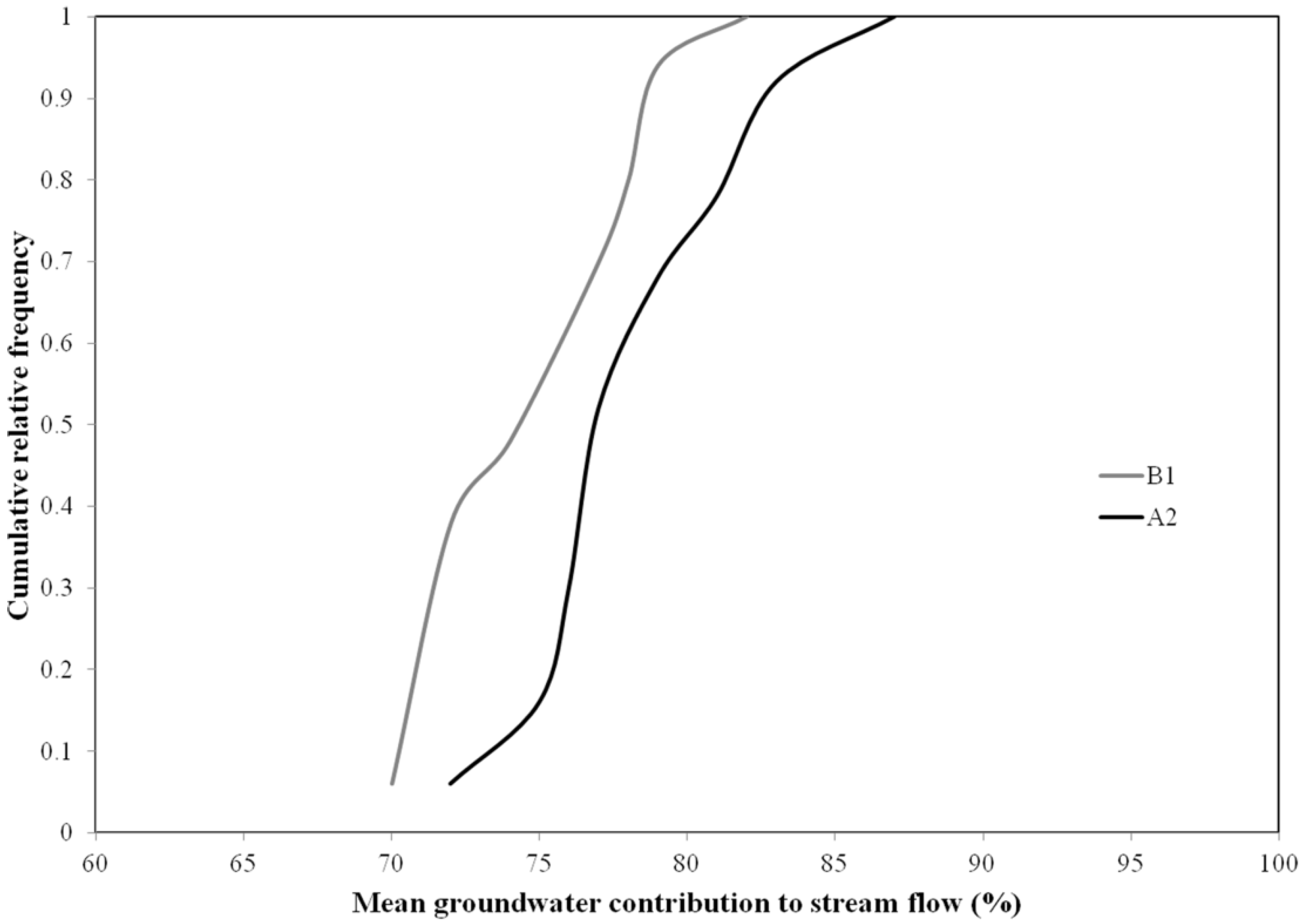
Figure 6 illustrates the cumulative relative frequency distribution of the mean annual groundwater contribution to stream flow in 2013 under the A2 and B1 scenarios. Similar to the pattern of the cumulative relative frequency distribution of mean monthly groundwater contributions to stream flow, the pattern of the cumulative relative frequency distribution of mean annual groundwater contributions to stream flow under both scenarios varied due to the modeling parameter uncertainty. Under the A2 scenario, the mean annual groundwater contribution to stream flow ranged from 72% to 87%, with a mean of 79% and a standard deviation of 4%. On the other hand, the mean annual groundwater contribution to stream flow in 2013 was 78% using the calibrated parameters’ values. Under the B1 scenario, the mean annual groundwater contribution to stream flow ranged from 70% to 82%, with a mean of 75% and a standard deviation of 3.5%. On the other hand, the mean annual groundwater contribution to stream flow in 2013 was close to 77% using the calibrated parameters’ values. Compared to the A2 scenario, the range of the mean annual groundwater contributions to stream flow under the B1 scenario was lower. This occurred because more precipitation was predicted under the B1 scenario than under the A2 scenario in 2013. This increased precipitation resulted in surface water and groundwater levels increasing. However, the major increase occurred in surface water levels due to increased surface runoff because of the steep topography of the study area (average slope of 7.8%). Therefore, the gradient between the groundwater and surface water was decreased, and resulted in lower range of mean annual groundwater contribution to stream flow under the B1 scenario. It also demonstrated that uncertainty in the mean annual groundwater contribution to the stream flow under the A2 scenario was higher than that in the B1 scenario because of the higher precipitation in the B1 scenario. Therefore, lower uncertainties are associated in GW-SW interaction system during wet years compared to dry years. This reflects the complexities in GW-SW interaction system.
The uncertainty analysis provides a range of outputs instead of one output, and this range of outputs would provide more information to the watershed manager to take particular action with a certain degree of risks regarding water withdrawal from the river and allocation to stakeholders for future water supplies depending on the month and season. However, the range of outputs and prediction would differ from year to year depending on the amount and pattern (i.e., only rainfall or both snow and rainfall) of the annual precipitation.
5. Conclusions
In this study an uncertainty analysis of GW-SW interaction was conducted to understand and determine the variation of temporal (i.e., monthly, and annual) mean groundwater contributions to stream flow due to parameter uncertainty by using a new technique, which was based on temporal mean groundwater contributions to streamflow. The uncertainty analysis results showed that the pattern of the cumulative relative frequency distribution of mean monthly and annual groundwater contributions to stream flow under both case scenarios varied monthly and annually, respectively, because of the uncertainties of the sensitive model parameters. The results also demonstrated that uncertainties in the sensitive parameters had significant effects on the predicted mean monthly and annual groundwater contributions to stream flow. The comparison of two case scenarios also indicated that lower uncertainties are associated in the GW-SW interaction system during wet years compared to dry years. In general, these uncertainty analysis results represent a new way to indicate the complexities and uncertainties in GW-SW interaction system. Therefore, it is very essential to use the uncertainty analysis results for better water resources management decision-making.
Acknowledgments
The authors would like to thank two anonymous reviewers for providing their valuable comments and suggestions, which contributed much to improve the paper. The authors would also like to thank Peter Caputa, Faye Hirshfield, Siddhartho Shekhar Paul, Malyssa Maurer, Reg Whiten, and Chelton van Geloven for their help and support.
Author Contributions
Gopal Chandra Saha and Jianbing Li designed the idea; Gopal Chandra Saha performed the simulation, and analyzed the results; Gopal Chandra Saha, Jianbing Li, and Ronald W. Thring wrote the paper.
Conflicts of Interest
The authors have declared that no competing interests exist.
References
- Kalbus, E.; Reinstorf, F.; Schirmer, M. Measuring methods for groundwater-surface water interactions: A review. Hydrol. Earth Syst. Sci. 2006, 10, 873–887. [Google Scholar] [CrossRef]
- Sophocleous, M. Interactions between groundwater and surface water: The state of the science. Hydrogeol. J. 2002, 10, 52–67. [Google Scholar] [CrossRef]
- Scibek, J.; Allen, D.M. Modeled impacts of predicted climate change on recharge and groundwater levels. Water Resour. Res. 2006, 42, W11405. [Google Scholar] [CrossRef]
- Van Roosmalen, L.; Christensen, B.S.B.; Sonnenborg, T.O. Regional differences in climate change impacts on groundwater and stream discharge in Denmark. Vadose Zone J. 2007, 6, 554–571. [Google Scholar] [CrossRef]
- Goderniaux, P. Impact of climate change on groundwater reserves. Ph.D. Thesis, University of Liege, Liège, Belgium, 2010. [Google Scholar]
- Stoll, S.; Hendricks Franssen, H.J.H.; Butts, M.; Kinzelbach, W. Analysis of the impact of climate change on groundwater related hydrological fluxes: A multi-model approach including different downscaling methods. Hydrol. Earth Syst. Sci. 2011, 15, 21–38. [Google Scholar] [CrossRef]
- Jackson, C.R.; Meister, R.; Prudhomme, C. Modeling the effects of climate change and its uncertainty on UK Chalk groundwater resources from an ensemble of global climate model projections. J. Hydrol. 2011, 399, 12–28. [Google Scholar] [CrossRef]
- Vansteenkiste, T.; Tavakoli, M.; Ntegeka, V.; Willems, P.; De Smedt, F; Batelaan, O. Climate change impact on river flows and catchment hydrology: A comparison of two spatially distributed models. Hydrol. Process. 2012. [Google Scholar] [CrossRef]
- El Hassan, A.A.; Sharif, H.O.; Jackson, T.; Chintalapudi, S. Performance of a conceptual and physically based model in simulating the response of a semi-urbanized watershed in San Antonio, Texas. Hydrol. Process. 2013, 27, 3394–3408. [Google Scholar] [CrossRef]
- Wu, B.; Zheng, Y.; Tian, Y.; Wu, X.; Yao, Y.; Han, F.; Liu, J.; Zheng, C. Systematic assessment of the uncertainty in integrated surface water-groundwater modeling based on the probabilistic collocation method. Water Resour. Res. 2014, 50, 5848–5865. [Google Scholar] [CrossRef]
- Faramarzi, M.; Abbaspour, K.C.; Adamowicz, W.L.; Lu, W.; Fennell, J.; Zehnder, A.J.B.; Goss, G.G. Uncertainty based assessment of dynamic freshwater scarcity in semi-arid watersheds of Alberta, Canada. J. Hydrol. Reg. Stud. 2017, 9, 48–68. [Google Scholar] [CrossRef]
- Benke, K.K.; Lowell, K.E.; Hamilton, A.J. Parameter uncertainty, sensitivity analysis and prediction error in a water-balance hydrological model. Math. Comput. Model. 2008, 47, 1134–1149. [Google Scholar] [CrossRef]
- Muleta, M.K.; Nicklow, J.W. Sensitivity and uncertainty analysis coupled with automatic calibration for a distributed watershed model. J. Hydrol. 2004, 306, 127–145. [Google Scholar] [CrossRef]
- Beven, K.J.; Binley, A.M. The future of distributed models: Model calibration and uncertainty prediction. Hydrol. Process. 1992, 6, 279–298. [Google Scholar] [CrossRef]
- Kuczera, G.; Mroczkowski, M. Assessment of hydrological parameter uncertainty and the worth of multiresponse data. Water Resour. Res. 1998, 34, 1481–1489. [Google Scholar] [CrossRef]
- Vrugt, J.A.; Gupta, H.V.; Bouten, W.; Sorooshian, S. A Shuffled Complex Evolution Metropolis algorithm for optimization and uncertainty assessment of hydrologic model parameters. Water Resour. Res. 2003, 39, 1201. [Google Scholar] [CrossRef]
- Mishra, S. Uncertainty and sensitivity analysis techniques for hydrologic modeling. J. Hydroinform. 2009, 11, 282–296. [Google Scholar] [CrossRef]
- Shen, Z.Y.; Chen, L.; Chen, T. Analysis of parameter uncertainty in hydrological and sediment modeling using GLUE method: A case study of SWAT model applied to Three Gorges Reservoir Region, China. Hydrol. Earth Syst. Sci. 2012, 16, 121–132. [Google Scholar] [CrossRef]
- Shen, Z.Y.; Chen, L.; Chen, T. The influence of parameter distribution uncertainty on hydrological and sediment modeling: A case study of SWAT model applied to the Daning watershed of the Three Gorges Reservoir Region, China. Stoch. Env. Res. Risk 2013, 27, 235–251. [Google Scholar]
- Fan, Y.R.; Huang, W.; Huang, G.H.; Huang, K.; Zhou, X. A PCM-based stochastic hydrological model for uncertainty quantification in watershed systems. Stoch. Env. Res. Risk 2015, 29, 915–927. [Google Scholar] [CrossRef]
- Fan, Y.R.; Huang, G.H.; Baetz, B.W.; Li, Y.P.; Huang, K.; Li, Z.; Chen, X.; Xiong, L.H. Parameter uncertainty and temporal dynamics of sensitivity for hydrologic models: A hybrid sequential data assimilation and probabilistic collocation method. Environ. Modell. Softw. 2016, 86, 30–49. [Google Scholar] [CrossRef]
- Wu, M.; Jansoon, P.; Tan, X.; Wu, J.; Huang, J. Constraining Parameter Uncertainty in Simulations of Water and Heat Dynamics in Seasonally Frozen Soil Using Limited Observed Data. Water 2016, 8, 64. [Google Scholar] [CrossRef]
- Naumburg, E.; Mata-Gonzalez, R.; Hunter, R.; Mclendon, T.; Martin, D. Phreatophytic vegetation and groundwater fluctuations: A review of current research and application of ecosystem response modeling with an emphasis on Great Basin vegetation. Environ. Manag. 2005, 35, 726–740. [Google Scholar] [CrossRef] [PubMed]
- Dobson Engineering Ltd.; Urban Systems Ltd. Kiskatinaw River Watershed Management Plan. 2003. File 0714.0046.01. Available online: http://www.dawsoncreek.ca/cityhall/departments/water/watershed/background-watershed-management-plans/ (accessed on 12 November 2016).
- Saha, G.C. Groundwater-surface water interaction under the effects of climate and land use changes. Ph.D. Thesis, University of Northern British Columbia, Prince George, BC, Canada, 2014. [Google Scholar]
- Saha, G.C.; Paul, S.S.; Li, J.; Hirshfield, F.; Sui, J. Investigation of land-use change and groundwater-surface water interaction in the Kiskatinaw River Watershed, British Columbia (parts of NTS 093P/01, /02, /07-/10) Report 2013-1. In Geoscience BC Summary of Activities 2012; Geoscience BC: Vancouver, BC, Canada, 2013; pp. 139–148. [Google Scholar]
- Ogden, F.L.; Saghafian, B. Green and ampt infiltration with redistribution. J. Irrig. Drain. Eng. 1997, 123, 386–393. [Google Scholar] [CrossRef]
- Downer, C.W. Identification and modeling of important stream flow producing processes in watersheds. Ph.D. Thesis, University of Connecticut, Storrs, USA, 2002. [Google Scholar]
- GeoBase. Available online: www.geobase.ca (accessed on 15 January 2016).
- Paul, S.S. Analysis of land use and land cover change in Kiskatinaw River watershed: A remote sensing, GIS & modeling approach. M.Sc. Thesis, University of Northern British Columbia, Prince George, BC, Canada, 2013. [Google Scholar]
- Land Resource Research Institute. Soils of Fort St. John-Dawson Creek, British Columbia. Soil Survey report No. 42; Agriculture Canada: Vancouver, BC, USA, 1985. [Google Scholar]
- Woldeamlak, S.T.; Batelaan, O.; De Smedt, F. Effects of climate change on the groundwater system in the Grote-Nete catchment, Belgium. Hydrogeol. J. 2007, 15, 891–901. [Google Scholar] [CrossRef]
- Solinst. Available online: www.solinst.com (accessed on 20 May 2014).
- McWhorter, D.B.; Sunada, D.K. Ground-water Hydrology and Hydraulics; Water Resources Publications: Fort Collins, Colorado, USA, 1977. [Google Scholar]
- Kala Groundwater Consulting Ltd. Groundwater potential evaluation Dawson Creek. British Columbia. Reference. 2001, R01332-0622. Available online: http://www.dawsoncreek.ca/wordpress/wpcontent/uploads/watershed/2001DCk_Kala_GWPotential.pdf (accessed on 18 July 2016).
- Santhi, C.; Arnold, J.G.; Williams, J.R.; Dugas, W.A.; Srinivasan, R.; Hauck, L.M. Validation of the SWAT model on a large river basin with point and nonpoint sources. J. Am. Water Resour. Assoc. 2001, 37, 1169–1188. [Google Scholar] [CrossRef]
- Van Liew, M.W.; Arnold, J.G.; Garbrecht, J.D. Hydrologic simulation on agricultural watersheds: Choosing between two models. Trans. ASAE 2003, 46, 1539–1551. [Google Scholar] [CrossRef]
- IPCC. IPCC Special Report. Emission Scenarios; Cambridge University Press: Cambridge, UK, 2000; p. 570. [Google Scholar]
- British Columbia Ministry of Energy and Mines. The status of exploration and development activities in the Montney Play region of northern BC. 2012. Available online: http://www.offshore- oilandgas.gov.bc.ca/OG/oilandgas/petroleumgeology/UnconventionalGas /Documents/C%20Adams.pdf (accessed on 19 December 2015).
- Bergström, S.; Carlsson, B.; Gardelin, M.; Lindström, G.; Pettersson, A.; Rummukainen, M. Climate change impacts on runoff in Sweden – assessments by global climate models, dynamical downscaling and hydrological modeling. Clim. Res. 2001, 16, 101–112. [Google Scholar] [CrossRef]
- Hay, L.E.; Wilby, R.L.; Leavesley, G.H. A comparison of delta change and downscaled GCM scenarios for three mountainous basins in the United States. J. Am. Water Resour. Assoc. 2000, 36, 387–398. [Google Scholar] [CrossRef]
- Xu, C.Y.; Widen, E.; Halldin, S. Modelling hydrological consequences of climate change -Progress and challenges. Adv. Atmos. Sci. 2005, 22, 789–797. [Google Scholar] [CrossRef]
- Andreasson, J.; Bergström, S.; Carlsson, B.; Graham, L.P.; Lindström, G. Hydrological Change - Climate change impact simulation for Sweden. J. Hum. Environ. 2004, 33, 228–234. [Google Scholar] [CrossRef]
- Graham, L.P.; Andréasson, J.; Carlsson, B. Assessing climate change impacts on hydrology from an ensemble of regional climate models, model scales and linking methods – a case study on the Lule River basin. Clim. Change 2007, 81, 293–307. [Google Scholar] [CrossRef]
- Van Roosmalen, L.; Christensen, J.H.; Butts, M.; Jensen, K.H.; Refsgaard, J.C. An intercomparison of regional climate model data for hydrological impact studies in Denmark. J. Hydrol. 2010, 380, 406–419. [Google Scholar] [CrossRef]
- IPCC. Climate Change 2007: The Physical Science Basis, Contribution of working Group I to the 4th assessment report (AR4) of the Intergovernmental Panel on Climate Change; Cambridge University Press: Cambridge, UK, 2007; p. 996. [Google Scholar]
- Saltelli, A. What is Sensitivity Analysis? In Sensitivity Analysis; Saltelli, A., Chan, K., Scott, E.M., Eds.; Wiley: New York, NY, USA, 2000. [Google Scholar]
- Hamby, D.M. A review of techniques for parameter sensitivity analysis of environmental models. Environ. Monit. Assess. 1994, 32, 135–154. [Google Scholar] [CrossRef] [PubMed]
- Downer, C.W.; Ogden, F.L. Gridded Surface Subsurface Hydrologic Analysis (GSSHA) User’s Manual; Version 1.43 for Watershed Modeling System 6.1; U.S. Army Engineer Research and Development Center: Vicksburg, MS, USA, 2006; ERDC/CHL SR-06-1.
- Rushton, K. Representation in regional models of saturated river-aquifer interaction for gaining/losing rivers. J. Hydrol. 2007, 334, 262–281. [Google Scholar] [CrossRef]
- Nejadhashemi, A.P.; Wardynski, B.J.; Munoz, J.D. Evaluating the impacts of land use changes on hydrologic responses in the agricultural regions of Michigan and Wisconsin. Hydrol. Earth Syst. Sci. Discuss. 2011, 8, 3421–3468. [Google Scholar] [CrossRef]
- Clapp, R.B.; Hornberger, G.M. Empirical equations for some soil hydraulic properties. Water Resour. Res. 1978, 14, 601–604. [Google Scholar] [CrossRef]
- Rawls, W.J.; Brakensiek, R.L.; Saxton, K.E. Estimation of soil water properties. Trans. ASAE 1982, 25, 1316–1320. [Google Scholar] [CrossRef]
- Rawls, W.J.; Brakensiek, D.L.; Miller, N. Green–Ampt infiltration parameters from soil data. J. Hydraul. Eng. 1983, 109, 62–70. [Google Scholar] [CrossRef]
- Reynolds, W.D.; Drury, C.F.; Yang, X.M.; Fox, C.A.; Tan, C.S.; Zhang, T.Q. Land management effects on the near-surface physical quality of a clay loam soil. Soil Tillage Res. 2007, 96, 316–330. [Google Scholar] [CrossRef]
- Minhas, P.S.; Sharma, D.R. Hydraulic conductivity and clay dispersion as affected by application sequence of saline and simulated rain water. Irrig. Sci. 1986, 7, 159–167. [Google Scholar]
- Miller, L.L.; Hinkel, K.M.; Nelson, F.E.; Paetzold, R.F.; Outcalt, S.I. Spatial and temporal patterns of soil moisture and thaw depth at barrow, Alaska USA. In Proceedings of the Seventh International Conference on Permafrost, Yellowknife, NT, Canada, 23-27 June 1998. Collection Nordicana No. 55. [Google Scholar]
- Bora, P.K.; Rajput, T.B.S. Spatial and temporal variability of manning’s n in irrigation furrows. J. Agric. Eng. 2003, 40, 35–42. [Google Scholar]
- Hatch, C.E.; Fisher, A.T.; Ruehl, C.R.; Stemler, G. Spatial and temporal variations in streambed hydraulic conductivity quantified with time-series thermal methods. J. Hydrol. 2010, 389, 276–288. [Google Scholar] [CrossRef]
- Saskatchewan Ministry of Agriculture. Irrigation scheduling manual. November 2008. Available online: http://www.agriculture.gov.sk.ca/Default.aspx?DN=288f45ad-5bab-41b1-9878-80acf555e3bf (accessed on 19 May 2013).
- Chen, X.; Mi, H.; He, H.; Liu, R.; Gao, M.; Huo, A.; Cheng, D. Hydraulic conductivity variation within and between layers of a high floodplain profile. J. Hydrol. 2014, 515, 147–155. [Google Scholar] [CrossRef]
- Cheng, C.; Song, J.; Chen, X.; Wang, D. Statistical Distribution of Streambed Vertical Hydraulic Conductivity along the Platte River, Nebraska. Water Resour. Manag. 2011, 25, 265–285. [Google Scholar] [CrossRef]
- Le, T.M.H.; Eiksund, G.R.; Strom, P.J. Statistical characterisation of soil porosity. In Safety, Reliability, Risk and Life-Cycle Performance of Structures and Infrastructures; Deodatis, G., Ellingwood, B.R., Frangopol, D.M., Eds.; Taylor & Francis Group: London, UK, 2013; pp. 5395–5402. [Google Scholar]
- Morikawa, H.; Iiyama, K.; Ohori, M. A study of the stochastic properties of auto-correlation coefficients for micrometer data simultaneously observed at two sites. In Applications of Statistics and Probability in Civil Engineering; Faber, M.H., Kohler, J., Nishijima, K., Eds.; Taylor & Francis Group: London, UK, 2011; pp. 723–727. [Google Scholar]
- Choi, M.; Jacobs, J.M. Soil moisture variability of root zone profiles within SMEX02 remote sensing footprints. Adv. Water Res. 2007, 30, 883–896. [Google Scholar] [CrossRef]
- Adams, J.R.; Berg, A.A.; McNairn, H. Field leve; soil moisture variability at 6- and 3-cm sampling depths: Implications for microwave sensor validation. Vadose Zone J. 2013, 12. [Google Scholar] [CrossRef]
- Lahkim, M.B.; Garcia, L.A. Stochastic modeling of exposure and risk in a contaminated heterogeneous aquifer, 1: Monte Carlo uncertainty analysis. Environ. Eng. Sci. 1999, 16, 315–328. [Google Scholar] [CrossRef]
- Clow, D.W.; Schrott, L.; Webb, R.; Campbell, D.H.; Torizzo, A.; Dornblaser, M. Groundwater occurrence and contributions to stream flow in an Alpine catchment, Colorado Front Range. Groundw.– Watershed Issue 2003, 41, 937–950. [Google Scholar] [CrossRef]
- Koeniger, P.; Leibundgut, C.; Stichler, W. Spatial and temporal characterization of stable isotopes in river water as indicators of groundwater contribution and confirmation of modelling results; a study of the Weser river, Germany. Isot. Environ. Health Stud. 2009, 45, 289–302. [Google Scholar] [CrossRef] [PubMed]
Figure 1.
Land use map of the study area and its location in the Kiskatinaw River Watershed, as well as in Canada.
Figure 1.
Land use map of the study area and its location in the Kiskatinaw River Watershed, as well as in Canada.
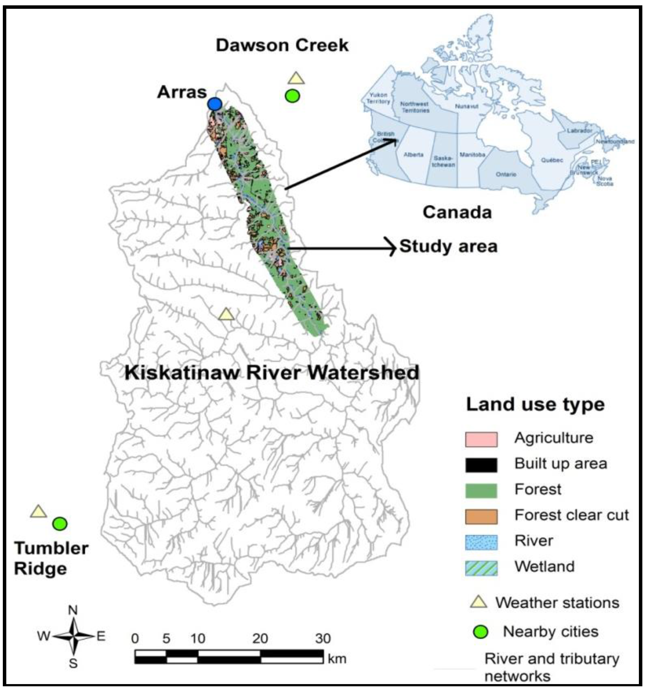
Figure 2.
Observed and simulated stream flows by the GSSHA model at the outlet of the study area during (a) calibration and (b) validation periods.
Figure 2.
Observed and simulated stream flows by the GSSHA model at the outlet of the study area during (a) calibration and (b) validation periods.
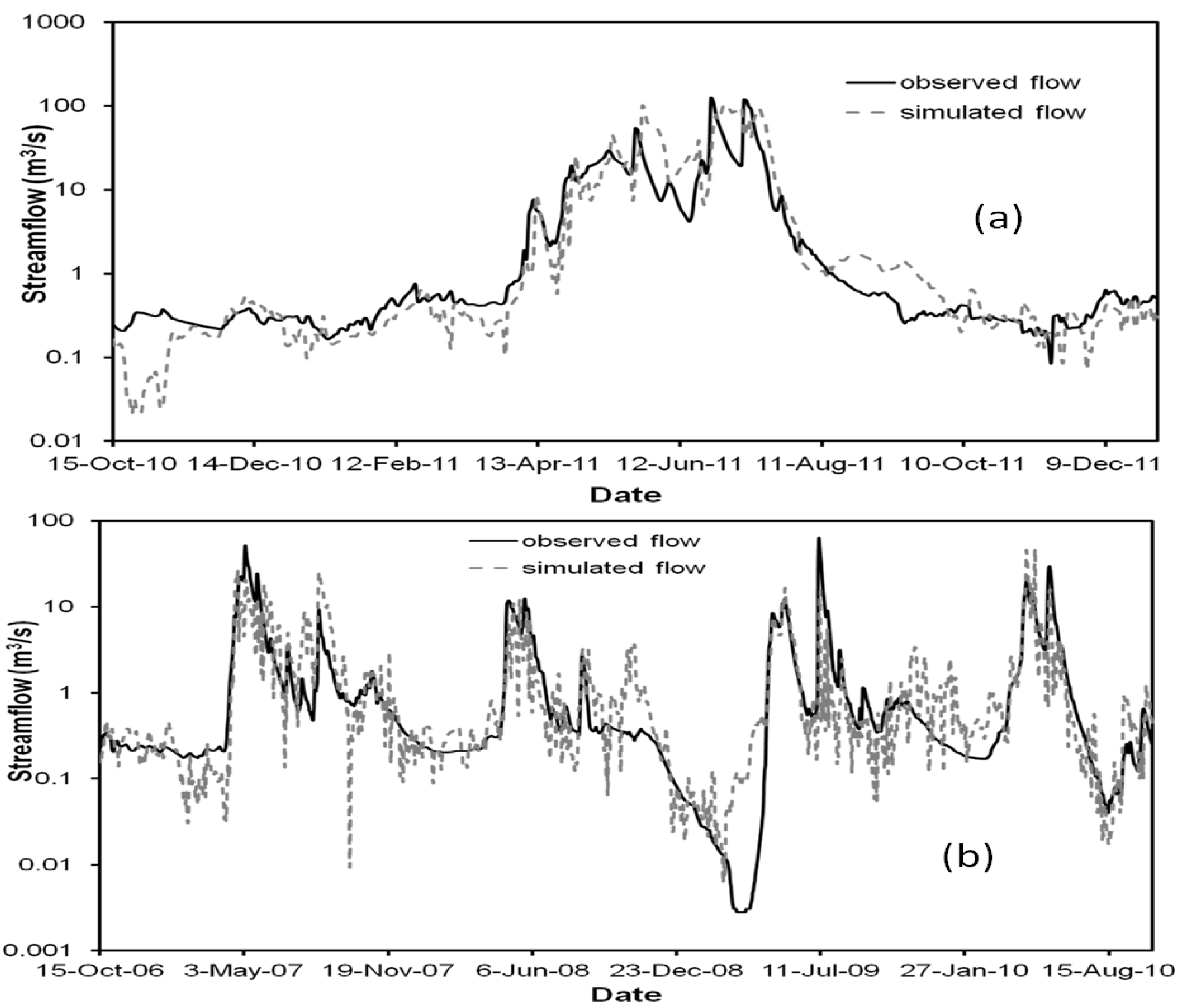
Figure 3.
Projected (a) mean monthly temperatures and (b) monthly precipitations under the A2 and B1 scenarios in 2013.
Figure 3.
Projected (a) mean monthly temperatures and (b) monthly precipitations under the A2 and B1 scenarios in 2013.
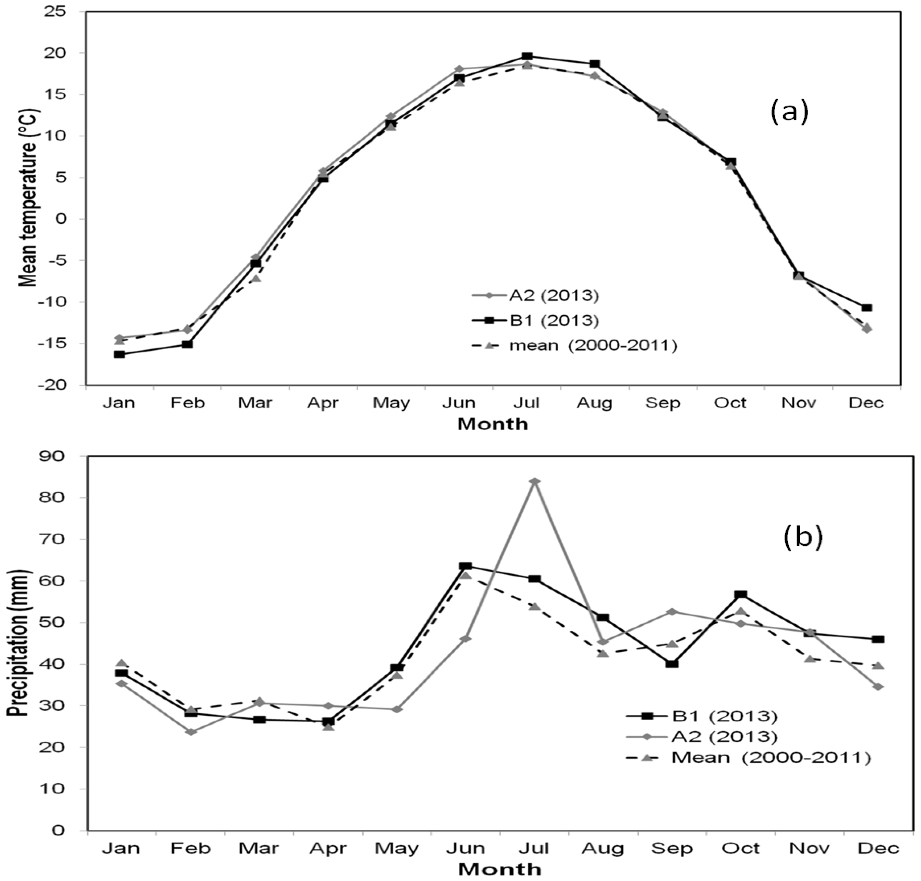
Figure 4.
Cumulative relative frequency distribution of mean groundwater contributions to stream flow in different months of 2013 under the A2 GHG emission scenario.
Figure 4.
Cumulative relative frequency distribution of mean groundwater contributions to stream flow in different months of 2013 under the A2 GHG emission scenario.
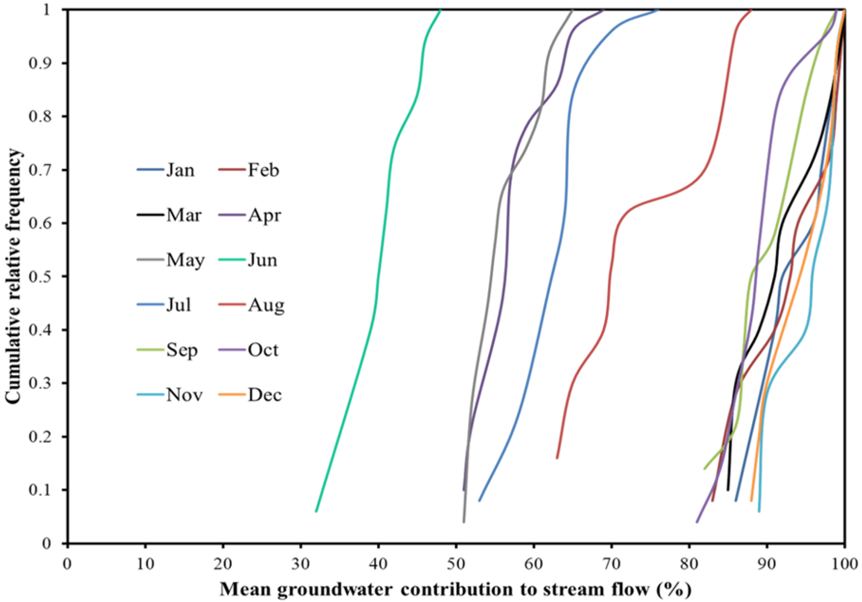
Figure 5.
Cumulative relative frequency distribution of mean groundwater contributions to stream flow in different months of 2013 under the B1 GHG emission scenario.
Figure 5.
Cumulative relative frequency distribution of mean groundwater contributions to stream flow in different months of 2013 under the B1 GHG emission scenario.
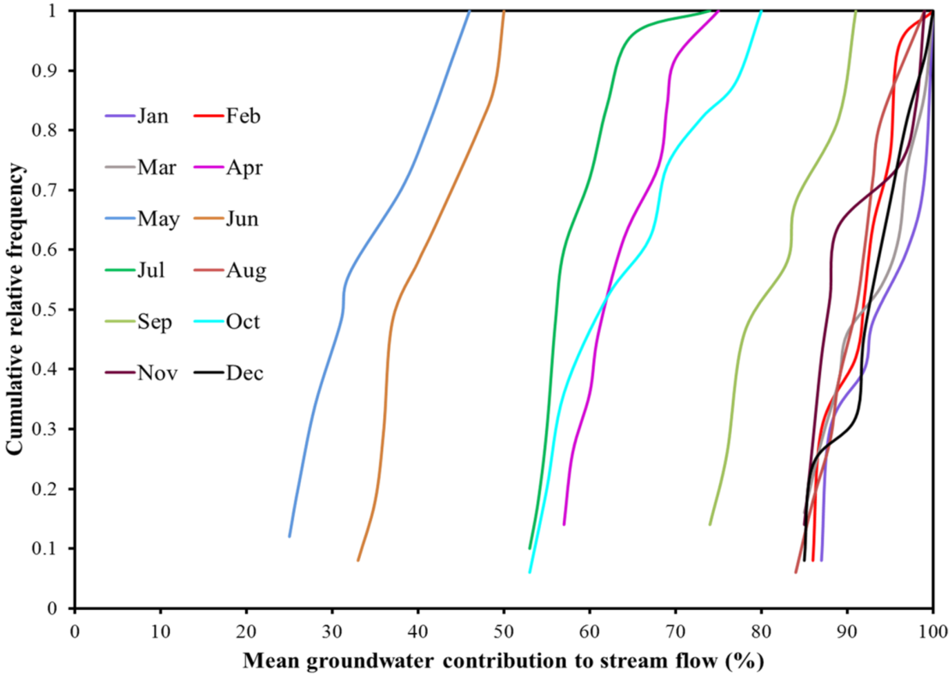
Figure 6.
Cumulative relative frequency distribution of mean annual groundwater contributions to the stream flow in 2013 under the A2 and B1 GHG emission scenarios.
Figure 6.
Cumulative relative frequency distribution of mean annual groundwater contributions to the stream flow in 2013 under the A2 and B1 GHG emission scenarios.


Table 1.
Details of input data for GSSHA model development.
| Data Type | Data and Format | Source |
|---|---|---|
| Watershed |
| |
| Hydrological |
|
|
| Climate and Meteorological |
|
|
Table 2.
Calibrated parameters’ values used in the GSSHA model. Here GW means groundwater.
| Process | Process Parameter | Unit | Value |
|---|---|---|---|
| Infiltration and GW | Saturated hydraulic conductivity (Ks) (clay loam-forest) | cm/hr | 0.15 |
| Infiltration and GW | Ks (clay loam-built-up area) | cm/hr | 0.03 |
| Infiltration and GW | Ks (clay loam-forest clear cut area) | cm/hr | 0.08 |
| Infiltration and GW | Ks (clay loam-agriculture) | cm/hr | 0.10 |
| Infiltration and GW | Ks (clay loam-wetland) | cm/hr | 0.05 |
| Infiltration and GW | Ks (sandy loam-forest) | cm/hr | 0.93 |
| Infiltration and GW | Ks (sandy loam-forest clear cut area) | cm/hr | 0.34 |
| Infiltration and GW | Ks (sandy loam-agriculture) | cm/hr | 0.42 |
| Infiltration and GW | Ks (silt loam-forest clear cut area) | cm/hr | 0.7 |
| Infiltration and GW | Ks (silt loam-forest) | cm/hr | 0.81 |
| Infiltration and GW | Ks (silt loam-built-up area) | cm/hr | 0.09 |
| Infiltration | Initial moisture (clay loam) | - | 0.21 |
| Infiltration | Initial moisture (silt loam) | - | 0.15 |
| Infiltration | Initial moisture (sandy loam) | - | 0.11 |
| Overland flow | Manning’s n (built-up area) | - | 0.011 |
| Overland flow | Manning’s n (agriculture) | - | 0.035 |
| Overland flow | Manning’s n (forest) | - | 0.1 |
| Overland flow | Manning’s n (forest clear cut area) | - | 0.03 |
| Infiltration and GW | Porosity (silt loam) | - | 0.501 |
| Infiltration and GW | Porosity (clay loam) | - | 0.464 |
| Infiltration and GW | Porosity (sandy loam) | - | 0.453 |
| Channel flow | Manning’s n (river) | - | 0.025 |
| Soil moisture | Soil moisture depth | m | 0.5 |
| GW-stream | Ks (stream bed material) | cm/hr | 1.1 |
| GW-stream | Stream bed material’s thickness | cm | 15 |
| Retention | Retention depth (agriculture) | mm | 0.1 |
| Retention | Retention depth (forest) | mm | 0.12 |
| Retention | Retention depth (forest clear cut area) | mm | 0.1 |
Table 3.
Calibrated parameters’ relative sensitivities and their sensitivity rankings.
| Parameter | Unit | Relative Sensitivity | Rank |
|---|---|---|---|
| Manning’s n (river) | - | 0.39 | 1 |
| Soil moisture depth | m | 0.32 | 2 |
| Initial soil moisture (clay loam) | - | 0.29 | 3 |
| Ks (clay loam-forest) | cm/hr | 0.24 | 4 |
| Porosity (clay loam) | - | 0.12 | 5 |
| Ks (clay loam-forest clear cut area) | cm/hr | 0.08 | 6 |
| Ks (clay loam-agriculture) | cm/hr | 0.006 | 7 |
| Ks (sandy loam-forest) | cm/hr | 0.0052 | 8 |
| Ks (clay loam-built up area) | cm/hr | 0.005 | 9 |
| Ks (clay loam-wetland) | cm/hr | 0.003 | 10 |
| Porosity (silt loam) | - | 0.002 | 11 |
| Ks (silt loam-forest) | cm/hr | 0.0001 | 12 |
Table 4.
Mean and standard deviation values of the most sensitive parameters used for uncertainty analysis.
Table 4.
Mean and standard deviation values of the most sensitive parameters used for uncertainty analysis.
| Parameter | Unit | Mean | Standard Deviation |
|---|---|---|---|
| Manning’s n (river) | - | 0.032 | 0.01 |
| Soil moisture depth | m | 0.60 | 0.125 |
| Initial soil moisture (clay loam) | - | 0.18 | 0.04 |
| Ks (clay loam-forest) | cm/hr | 0.20 | 0.08 |
| Porosity (clay loam) | - | 0.45 | 0.02 |
| Ks (clay loam-forest clear cut area) | cm/hr | 0.12 | 0.05 |
Table 5.
Uncertainty analysis results of mean monthly groundwater contributions to stream flow under the A2 GHG emission scenario in 2013 against the simulated value for corresponding month using the calibrated parameters’ values.
Table 5.
Uncertainty analysis results of mean monthly groundwater contributions to stream flow under the A2 GHG emission scenario in 2013 against the simulated value for corresponding month using the calibrated parameters’ values.
| Month | Range of Mean Groundwater Contribution to Stream Flow (%) | Mean (%) | Standard Deviation (%) | Output Using the Calibrated Parameters’ Values (%) |
|---|---|---|---|---|
| January | 86–100 | 94.19 | 5.74 | 93.16 |
| February | 83–100 | 93.22 | 6.32 | 90.79 |
| March | 85–100 | 92.44 | 5.63 | 93.53 |
| April | 51–69 | 58.19 | 6.08 | 54.26 |
| May | 51–65 | 56.78 | 4.71 | 57.23 |
| June | 32–48 | 41.10 | 4.45 | 44.04 |
| July | 53–76 | 64.40 | 5.55 | 59.20 |
| August | 63–88 | 76.76 | 10.01 | 71.89 |
| September | 82–99 | 90.41 | 6.33 | 88.94 |
| October | 81–99 | 90.06 | 5.53 | 93.81 |
| November | 89–99 | 94.73 | 4.35 | 95.90 |
| December | 88–100 | 95.23 | 4.55 | 97.50 |
Table 6.
Uncertainty analysis results of mean monthly groundwater contributions to stream flow under the B1 GHG emission scenario in 2013 against simulated value for corresponding month by using the calibrated parameters’ values.
Table 6.
Uncertainty analysis results of mean monthly groundwater contributions to stream flow under the B1 GHG emission scenario in 2013 against simulated value for corresponding month by using the calibrated parameters’ values.
| Month | Range of Mean Groundwater Contribution to Stream Flow (%) | Mean (%) | Standard Deviation (%) | Output Using the Calibrated Parameters’ Values (%) |
|---|---|---|---|---|
| January | 87–100 | 94.29 | 5.56 | 99.79 |
| February | 86–100 | 93.53 | 4.94 | 98.32 |
| March | 85–100 | 93.27 | 5.82 | 98.46 |
| April | 57–75 | 64.15 | 6.35 | 63.16 |
| May | 25–46 | 35.67 | 7.97 | 28.30 |
| June | 33–50 | 41.35 | 6.36 | 47.21 |
| July | 53–74 | 60.53 | 6.43 | 61.30 |
| August | 84–99 | 91.64 | 5.19 | 96.20 |
| September | 74–91 | 81.99 | 6.91 | 87.70 |
| October | 53–80 | 66.02 | 10.10 | 56.48 |
| November | 85–99 | 91.15 | 5.49 | 87.82 |
| December | 85–100 | 92.65 | 5.64 | 97.89 |
© 2017 by the authors. Licensee MDPI, Basel, Switzerland. This article is an open access article distributed under the terms and conditions of the Creative Commons Attribution (CC BY) license (http://creativecommons.org/licenses/by/4.0/).
Share and Cite
MDPI and ACS Style
Saha, G.C.; Li, J.; Thring, R.W. Understanding the Effects of Parameter Uncertainty on Temporal Dynamics of Groundwater-Surface Water Interaction. Hydrology 2017, 4, 28. https://doi.org/10.3390/hydrology4020028
AMA Style
Saha GC, Li J, Thring RW. Understanding the Effects of Parameter Uncertainty on Temporal Dynamics of Groundwater-Surface Water Interaction. Hydrology. 2017; 4(2):28. https://doi.org/10.3390/hydrology4020028
Chicago/Turabian StyleSaha, Gopal Chandra, Jianbing Li, and Ronald W. Thring. 2017. "Understanding the Effects of Parameter Uncertainty on Temporal Dynamics of Groundwater-Surface Water Interaction" Hydrology 4, no. 2: 28. https://doi.org/10.3390/hydrology4020028
Note that from the first issue of 2016, this journal uses article numbers instead of page numbers. See further details here.