
Numerical Tests of the Lookup Table Method in Solving Richards’ Equation for Infiltration and Drainage in Heterogeneous Soils


1
Department of Mathematics, Shahjalal University of Science & Technology, Sylhet 3100, Bangladesh
2
Institut National de la Recherche Scientique, Centre Eau Terre Environnement (INRS-ETE), Université du Québec, Quebec City, QC G1K 9A9, Canada
3
Department of Mathematics, University of Padova, Padova 35121, Italy
*
Author to whom correspondence should be addressed.
Hydrology 2017, 4(3), 33; https://doi.org/10.3390/hydrology4030033
Submission received: 6 May 2017
/
Revised: 12 June 2017
/
Accepted: 14 June 2017
/
Published: 22 June 2017
Abstract
:The lookup table option, as an alternative to analytical calculation for evaluating the nonlinear heterogeneous soil characteristics, is introduced and compared for both the Picard and Newton iterative schemes in the numerical solution of Richards’ equation. The lookup table method can be a cost-effective alternative to analytical evaluation in the case of heterogeneous soils, but it has not been examined in detail in the hydrological modeling literature. Three layered soil test problems are considered, and the robustness and accuracy of the lookup table approach are assessed for uniform and non-uniform distributions of lookup points in the soil moisture retention curves. Results from the three one-dimensional test simulations show that the uniform distributed option gives improved convergence and robustness for the drainage problem compared to the non-uniform strategy. On the other hand, the non-uniform technique can be chosen for test problems involving flow into initially dry layered soils.
1. Introduction
Richards’ equation is a standard, commonly-used approach for describing flow in partially-saturated porous media. The highly nonlinear nature of Richards’ equation, due to the dependence of the hydraulic conductivity and diffusivity on the moisture content, in combination with the non-trivial forcing conditions that are often encountered in engineering practice, makes Richards’ equation practically impossible to solve using analytical approaches except for a few special cases [1,2,3]. One of the numerous varieties of Richards’ equation is based on the pressure head () formulation, which is the most commonly-used because it has the advantage of being applicable to both saturated and unsaturated conditions and accommodating heterogeneous soils. In this approach, mass balance is guaranteed by evaluating the moisture content change in a time step directly from the change in the water pressure head [4]. In modeling unsaturated flow problems involving sharp wetting fronts, it has been shown to offer excellent mass balance [5]. This technique is simple to employ in head-based codes, requiring only an additional source term. However, this approach may encounter difficulties in stability and convergence for a sharp wetting front [6,7,8,9]. Other methods such as the switching algorithm are also proposed for better mass balance in simulating transitions between saturated and unsaturated conditions [10,11], and the predictor-corrector method [10,12] can also be used to simulate variably-saturated flow problems. A computationally-economic convergence approach based on using the pressure head as the primary variable has been proposed [13]. The pressure head form of Richards’ equation with the small change of throughout a time step is able to attain good mass balance.
Soil water characteristic functions, which are required to solve Richards’ equation, are difficult to measure adequately for soils with heterogeneous pore systems. Capturing the moisture content profile across boundaries between materials with different hydraulic properties implies simulation of the flow problem in heterogeneous media. This has proven to be a challenging task for numerical modellers. Several numerical algorithms have been proposed to handle the discontinuity of fluid content in layered soils [14,15,16]. Severe difficulties are encountered when the analytical expression for the derivative of moisture content is used in the numerical simulation of fluid flow problem [17]. This is due to the shape of the soil water capacity function and the relative hydraulic conductivity near saturation [9]. As a result, numerical accuracy can be affected significantly, as can the stability and rate of convergence of the numerical scheme. Therefore, to circumvent such difficulties, a proper choice of the estimation method of soil characteristic functions for heterogeneous porous media is required. In this study, we adopted the lookup table technique, which is an alternative to the analytical calculation of moisture curves.
In the numerical procedures for the solution of flow problems in variably-saturated porous media, much effort has been devoted to overcoming mass conservation errors, numerical diffusion and other inaccuracies that can be generated. The numerical solution of Richards’ equation is very challenging due to the nonlinear dependency of the moisture content on the pressure head, and it requires sophisticated numerical techniques to overcome convergence difficulties and poor computational efficiency [17,18,19]. For the numerical solution of Richards’ equation, it is convenient to decouple the issues of temporal and spatial accuracy. A variety of numerical models have been proposed on the basis of the finite difference, finite element and finite volume methods to simulate saturated-unsaturated flow [4,8,11,20,21,22,23]. In addition, most variably-saturated flow simulators currently in use are based on fixed spatial grids and either fixed time steps or an empirically-based adaptive time stepping method [4,24]. The numerical stability of the finite element models is improved by mass lumping since previous findings indicate that consistent mass formulation can cause numerical oscillations [4,25,26]. The importance of proper treatment of the time derivative for reliable numerical simulations has also been shown [4,27]. Typically-used time stepping schemes are the backward Euler and Crank–Nicolson schemes, and it has been demonstrated that the second order schemes are generally more effective than first-order schemes [28]. Other time stepping schemes used for Richards’ equation include the three-level Lees’ and implicit factored schemes [28].
In linearization schemes, the Picard and Newton iterative methods represent the most common approaches to solve numerically the nonlinear Richards’ equation, with the simpler Picard technique being the more popular of the two [14,29,30,31,32,33,34,35]. It has been shown that the iterative Newton scheme is quadratically convergent, while Picard converges linearly [28]. Moreover, the implementation of the Picard scheme is easier, computationally inexpensive and preserves symmetry of the discrete system of equations, whereas the Newton scheme generates a nonsymmetric system matrix. This factor is important in assessing the relative efficiency of the two schemes, since different storage and linear solver algorithms can be used to exploit these structural differences. In many cases, the Picard scheme converges well and more efficiently, but for cases of gravity drainage, complex time-varying boundary conditions, strongly nonlinear characteristic equations and saturated/unsaturated interfaces, it can fail to converge or it may converge very slowly [19].
In this paper, we investigate the lookup table approach to enhance the performance of the Picard and Newton iterative methods for cases where convergence difficulties are met, in particular for heterogeneous soils. The lookup table method can be a cost-effective alternative to analytical evaluation of the soil moisture retention curves, but its performance has not been examined in detail in the hydrological modeling literature. Numerical results for three test problems illustrate the circumstances under which the two iterative schemes can be expected to perform poorly and, thus, provide useful cases for investigating alternative schemes, such as lookup table evaluation of heterogeneous soil characteristics.
2. Richards’ Equation for Flow in Variably-Saturated Porous Media
Richards’ equation may be written in three standard forms, with either pressure head or moisture content as dependent variables. These three forms of the saturated-unsaturated flow equation are the “-based” form, “-based” form and the “mixed ()” form. We assume that the porous media and water are incompressible and that the air phase is infinitely mobile, so that the air pressure remains constant. Finally, in our formulation, any source or sink terms are handled as boundary conditions.
For one-dimensional vertical flow in unsaturated soils, the pressure head-based Richards’ equation is written as:
where is the pressure head [], is time [], denotes the vertical distance from reference elevation, assumed positive upward [], is the hydraulic conductivity [], is the specific fluid capacity [] and is the volumetric water content [].
Usually, the -based form is used for heterogeneous soils of both saturated and unsaturated flow conditions. However, this formulation generally exhibits very poor preservation of mass balance, unacceptable time-step limitations [26] and relatively slow convergence [36].
In contrast, the -based form is a conservation form by construction, i.e., it follows the mass conservation law. In this form, mass balance is improved significantly, and rapidly convergent solutions can be obtained. However, unfortunately, they are strictly limited to unsaturated conditions, since in a saturated condition, the water content becomes constant and approaches infinity. Furthermore, for multi-layered soils, cannot be guaranteed to be continuous across interfaces separating the layers. Thus, this form is useful only for homogeneous media [37].
2.1. Constitutive Relationship
To complete the model formulation of Richards’ equation, we must specify the constitutive relationship to describe the interdependence among fluid pressures, saturations and relative permeabilities. There are several mathematical relationships for the constitutive or soil water retention curves that are used in modeling. The most commonly-used relationships are the Brooks–Corey [38] and the van Genuchten [39] equations. These two models are described as follows:
2.1.1. The Brooks–Corey Model
The constitutive relationships proposed by Brooks and Corey [38] are given by:
where θs is the saturated moisture content [], θr is the residual moisture content [], is the bubbling or air entry pressure head [L] and is equal to the pressure head to desaturate the largest pores in the medium and is a pore-size distribution index (dimensionless).
2.1.2. The Van Genuchten Model
Perhaps the most widely-used constitutive relations for moisture content and hydraulic conductivity are those of van Genuchten [39]. The model is given by:
2.2. Spatial Discretization
For the numerical solution of Richards’ equation (1), we discretize the spatial domain using the finite element Galerkin scheme and the time derivative term using a finite difference scheme. To develop the finite element model, there are discretized elements for M global nodes in the problem domain.
The approximating function is:
where and are linear Lagrange basis functions and nodal values of at time t, respectively. The method of weighted residuals is used to set the criteria to solve for the unknown coefficients. In local coordinate space , the approximating function for each element (e) is , which we can write in vector form as . The global function (14) becomes:
The symmetric weak formulation of Galerkin’s method applied to (1) yields the system of ordinary differential equations [18]:
where is the vector of undetermined coefficients corresponding to the values of pressure head at each node, A is the stiffness matrix, F is the storage or mass matrix, q contains the specified Darcy flux boundary conditions and b contains the gravitational gradient component. Over local subdomain element , we have:
Here, denotes the transpose of N.
2.3. Time Differencing
Equation (16) can be integrated by the weighted finite difference scheme. We obtain:
where , with ( is a weighting parameter) and and denote the previous and current time levels.
The time step size to ensure a stable solution will be dependent on the spatial discretization, and for nonlinear equations, there will in general also be a dependency on the form of the solution itself at any given time. Equation (20) is accurate, except for . When , the discretized scheme (20) corresponds to the Crank–Nicolson scheme.
The system of equations (20) is nonlinear in , except when , which corresponds to an explicit Euler scheme. When , the scheme becomes implicit. Some iteration or linearization strategy is thus needed to solve the system of nonlinear equations for the implicit case. For , the scheme corresponds to the backward Euler scheme.
Consider:
To linearize the nonlinear System (21), the most common iterative schemes are Picard and Newton. The Picard iterative scheme is more popular than Newton because the formulation of Picard is simple, and it preserves the symmetry of the finite element matrices. On the other hand, the Newton method requires the evaluation of Jacobian matrices and yields a nonsymmetric system. Because of this, the Picard method is less costly, on a per iteration basis, than the Newton method. The Picard method converges linearly, whereas Newton converges quadratically. Therefore, for some problems or under certain accuracy constraints, Newton gives better convergence behavior than Picard [19].
2.4. Newton Scheme
Applied to (21), the Newton scheme [28] can be written as:
where the superscripts m and m + 1 denote the previous and current iteration levels. The Jacobian for the system is:
expressed here in terms of ij-th component of the Jacobian matrix .
2.5. Picard Scheme
The Picard scheme has a simple formulation that can be obtained directly from (20) by iterating with all linear occurrences of taken at the current iteration level m + 1 and all nonlinear occurrences at the previous level m [28]. We get:
If we compare Equations (22) and (24), it can be seen that the Picard scheme is an approximation of Newton’s method. The linearization of Newton produces a nonsymmetric system matrix, whereas Picard yields a symmetric system. Since different storage and linear solver algorithms can be used to exploit these structural differences, this factor is very important to assess the relative efficiency of the two schemes. For the Newton scheme, we need to evaluate three derivative terms in the Jacobian, implying that the Newton scheme is more costly and algebraically complex than Picard.
3. Methodology
To investigate the performance of the lookup table option of the subsurface flow model used in this study [19], we consider three one-dimensional numerical test problems, the first two involving vertical drainage through a layered soil from initially-saturated conditions and the third involving one-dimensional flow into an initially very dry layered soil of sand and clay. There is a sharp region produced in the moisture capacity and relative hydraulic conductivity curves for these test problems. We examined the performance of the lookup table scheme in two ways: uniform and non-uniform distributions of lookup points in the domain of the constitutive relationship curves for both the Newton and Picard iterative schemes. Simple equally-spaced discretization of the moisture capacity, water saturation, relative hydraulic conductivity and other retention curves is defined for the uniform distributions of lookup table points. We have taken many points where the retention curves are very sharp, and fewer points are used where the curves are varying less for the non-uniform distribution case.
Dynamic time step sizes are adjusted according to the convergence behavior of the nonlinear iteration scheme. During any time step, a nonlinear convergence tolerance is specified, along with a maximum number of iterations, maxit (= 10). The starting simulation time step size is and continues until we reach the simulation time . If the convergence is achieved in a fewer number of iterations than another pre-assigned number of iterations , then the current time step size is increased by a specified magnification factor, denoted by , and this is repeated until we reach the maximum time step size . It remains unchanged if the convergence required falls between and iterations. The time step size is decreased by a reduction factor to a minimum step size if the convergence required less than . If convergence is not achieved within the maximum number of iterations, then back-stepping occurs, that is the solution is recomputed at the current time level using a smaller time step, reduced by the factor to a minimum size of . The infinity norm is used as the convergence termination criterion for both the Newton and Picard methods, that is when is satisfied then convergence is achieved.
All simulations were performed with the CATHY (CATchment HYdrology) model [19,40], which is a physically-based hydrological model where the surface module resolves the one-dimensional diffusion wave equation and the subsurface module solves the three-dimensional Richards’ equation. All runs were executed on a Dell Inspiron 2.56-GHz laptop computer.
4. Results
4.1. Test Problem 1
The main purposes of this first test case are: (i) to verify that we have correctly implemented the lookup table method (i.e., that it produces the same solutions as analytical evaluation of the nonlinear soil characteristics); (ii) to assess whether the lookup table method is robust (i.e., that it produces accurate solutions over a range of discretizations, as well as for varying numbers and distributions of lookup points); and (iii) to compare the computational efficiency and accuracy (mass balance error) of the lookup table approach against the analytical approach. This assessment is carried out by considering a one-dimensional vertical drainage through a layered soil of 2 m in depth from initially saturated conditions. Initially, the pressure head at the base of the column is reduced from 200 cm to 0 cm. During the subsequent drainage, for a duration of 12.15 d (1,050,000 s), a no flow boundary condition is imposed at the top, and a Dirichlet boundary condition is imposed at the base of the column. The domain of the soil column is parameterized by the van Genuchten relationships. The hydraulic properties of the soils are given in Table 1. The soil layers have different saturated hydraulic conductivity (Ks), but the same values for the van Genuchten parameters (θs, θr, α and n). The soil profile is Soil 1 for 0 < z < 80 cm and 140 cm < z < 200 cm and Soil 2 for 80 cm < z < 140 cm.
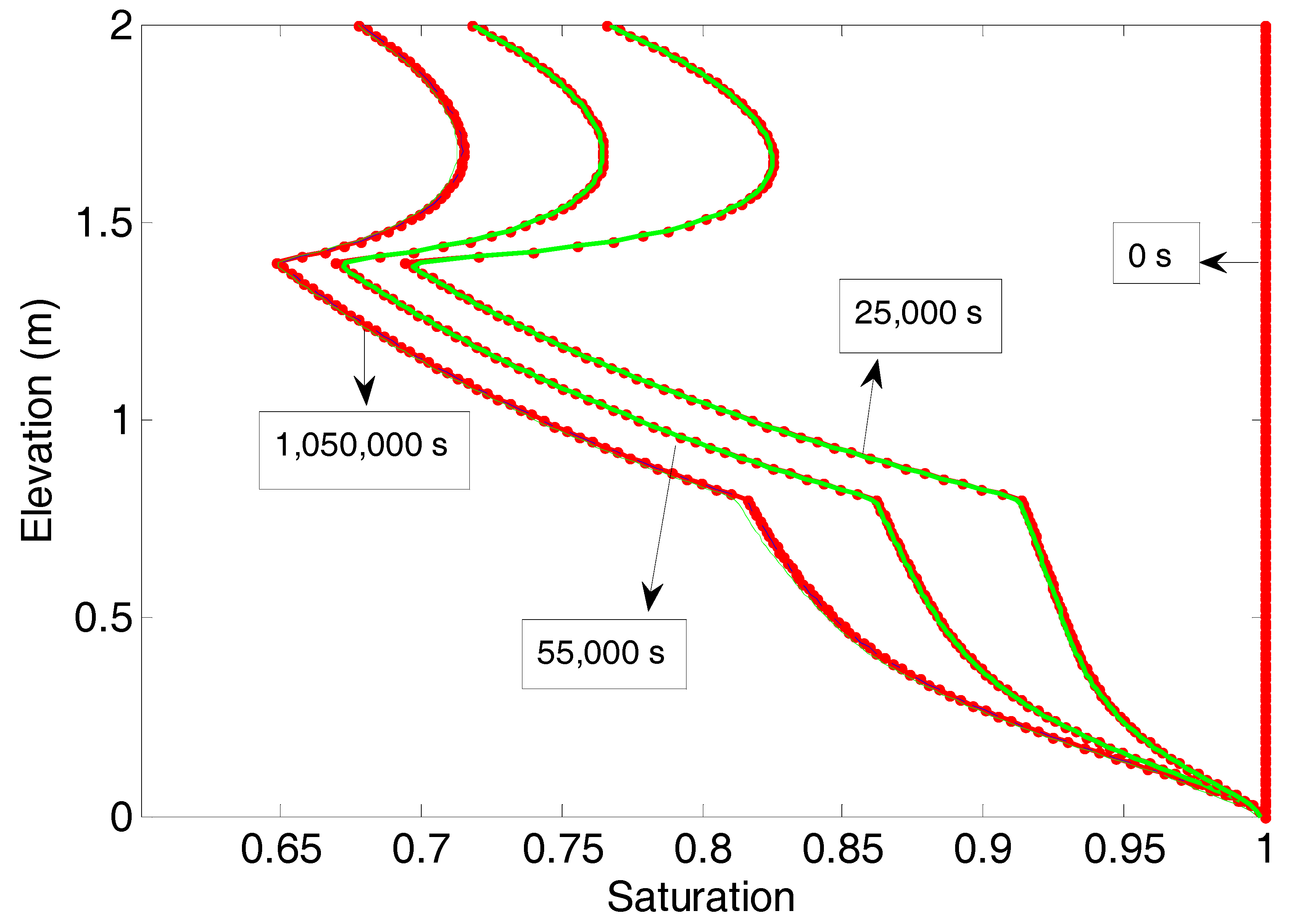
To obtain the analytical and lookup numerical solutions, the flow domain is discretized using two uniform grids consisting of 50 and 150 layers. The time discretizations are performed in a simple manner using a constant value s and 1000 s. The numerical results for this problem are obtained using Picard iteration and with 31 and 151 as the number of lookup points (NLKP) distributed both uniformly and non-uniformly for each set of layer and time step discretizations. Figure 1 shows the saturation profiles at four different times, at the start of drainage (0 s), at 250,000 s (2.9 d), at 550,000 s (6.4 d) and at 1,050,000 s (12.15 d), for both the analytical and lookup table approaches for the 150-layer, s discretization case. A very good agreement is exhibited between the analytical and lookup table results for both NLKP values, showing the accuracy of the lookup table approach even for a relatively small number of lookup points. Table 2 shows that the lookup table approach performs consistently (high accuracy) for all combinations of temporal and grid discretization and the number and distribution of lookup points. It is also of the same order of efficiency as the analytical approach (slightly better than analytical for NLKP = 31 and slightly worse for NLKP = 151).
4.2. Test Problem 2
For Test Cases 2 and 3, we will focus solely on the lookup table approach in order to examine its performance under different configurations. Unlike the first test case, Test Problems 2 and 3 will feature heterogeneity not only in Ks, but also in the retention curve parameters. Indeed, Test Problem 2 is identical to Test Problem 1, but with different layer thicknesses and with the addition of heterogeneity in the soil moisture retention curves, represented this time with the Brooks–Corey model. This problem is considered to be a challenging test for numerical methods because a sharp discontinuity in the moisture content occurs at the interface between two material layers [41,42,43]. During downward draining, the middle coarse soil tends to restrict drainage from the upper fine soil, and high saturation levels are maintained in the upper fine soil for a considerable period of time. The hydraulic properties of the soils are given in Table 3. The soil profile is Soil 1 for 0 < z < 60 cm and 120 cm < z < 200 cm and Soil 2 for 60 cm < z < 120 cm.
To compare the performance between the uniform and non-uniform distributions of lookup points, a fine mesh of 150 elements and a coarser mesh of 50 elements with two time step sizes ( = 100 s and 1000 s) and two sets of lookup table points (NLKP = 31 and 151) in the domain of the moisture curves are considered. Eight runs were performed for each of the iteration schemes (Picard and Newton).
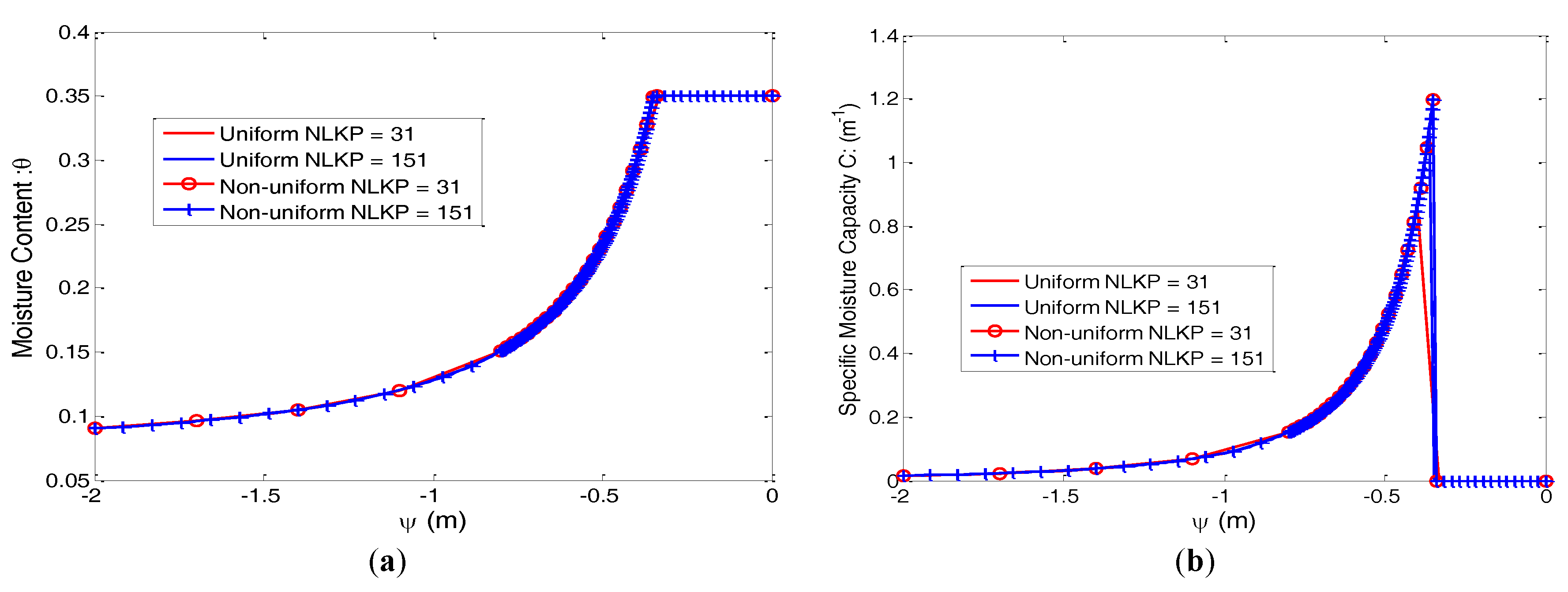
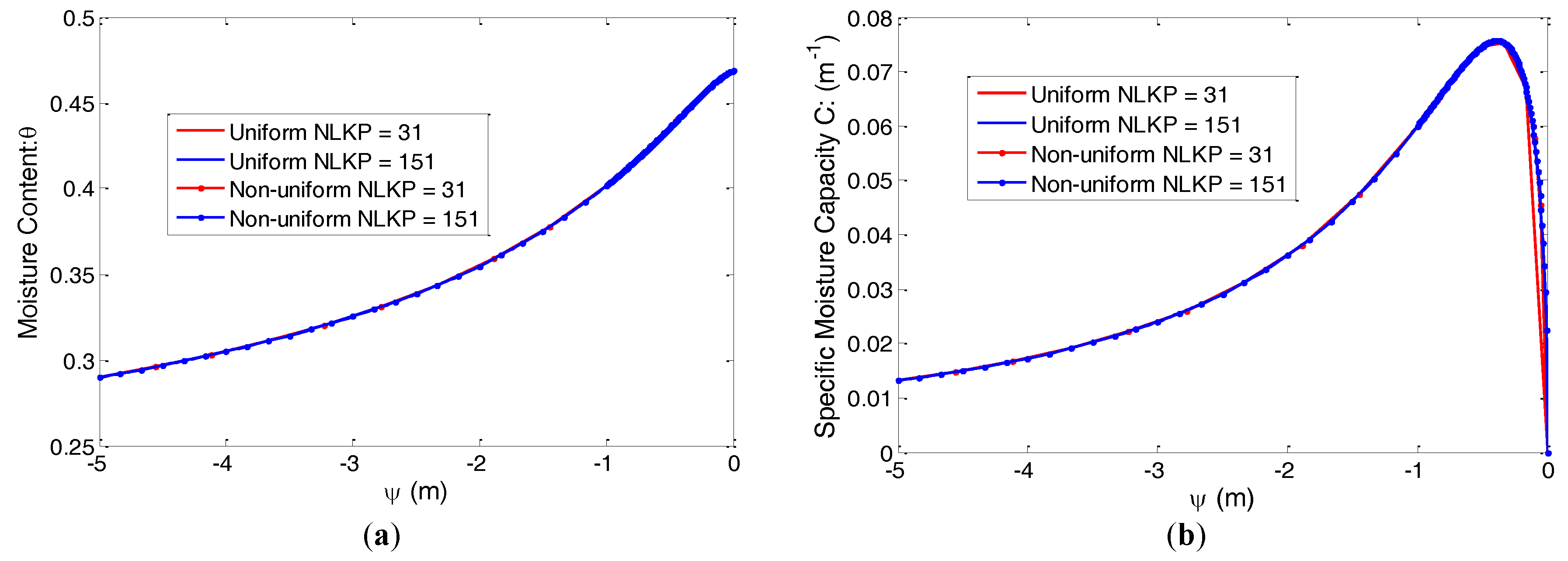
The soil moisture curves of the moisture content () and specific moisture capacity () for the uniform and non-uniform distribution of lookup points evaluated by the Brooks–Corey model are presented in Figure 2 (Soil 1) and Figure 3 (Soil 2). Highly nonlinear natures are clearly shown in the illustrated figures and make good challenges for a numerical algorithm.
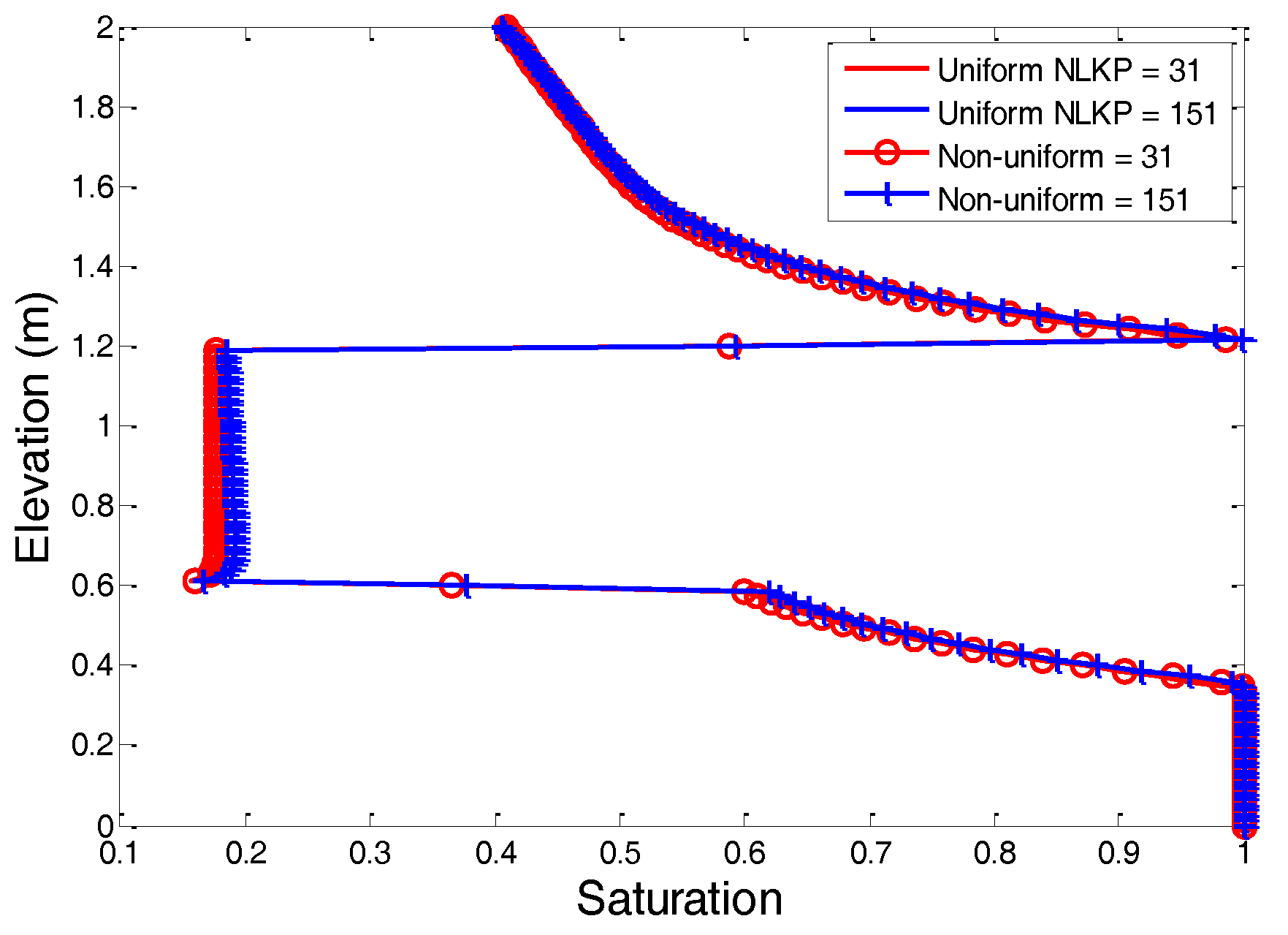
Figure 4 shows the saturation profiles at time 12.15 days for the various combinations simulated with the Picard scheme. It is shown that the solutions for 31 and 151 uniform and non-uniform lookup table points coincide very well. This implies that for the soil moisture retention curves, 31 lookup points are sufficient to obtain an efficient numerical solution of Richards’ equation.
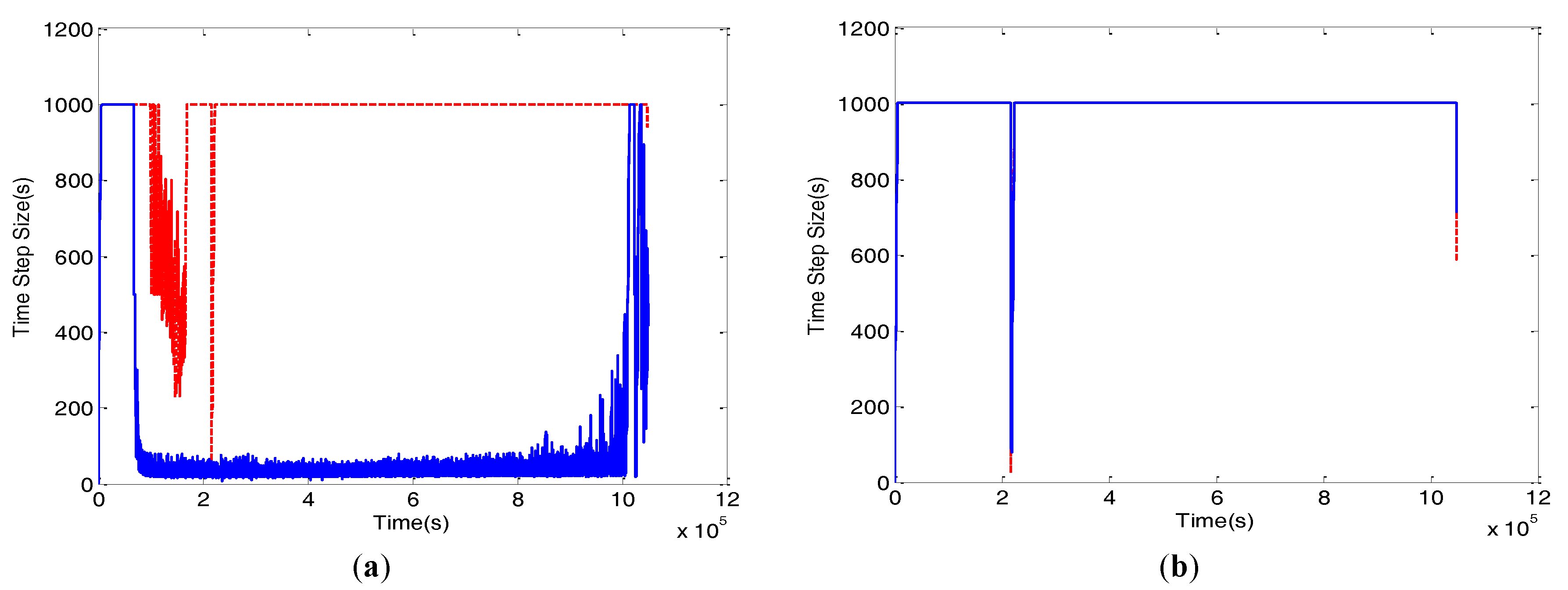
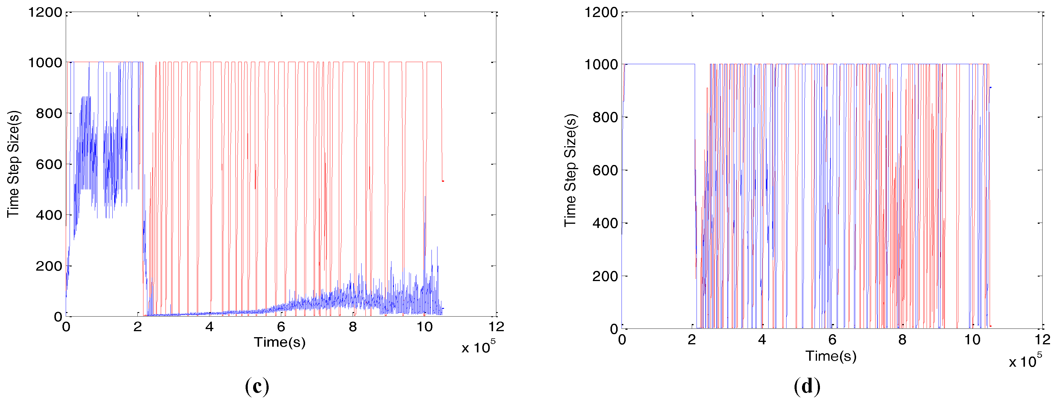
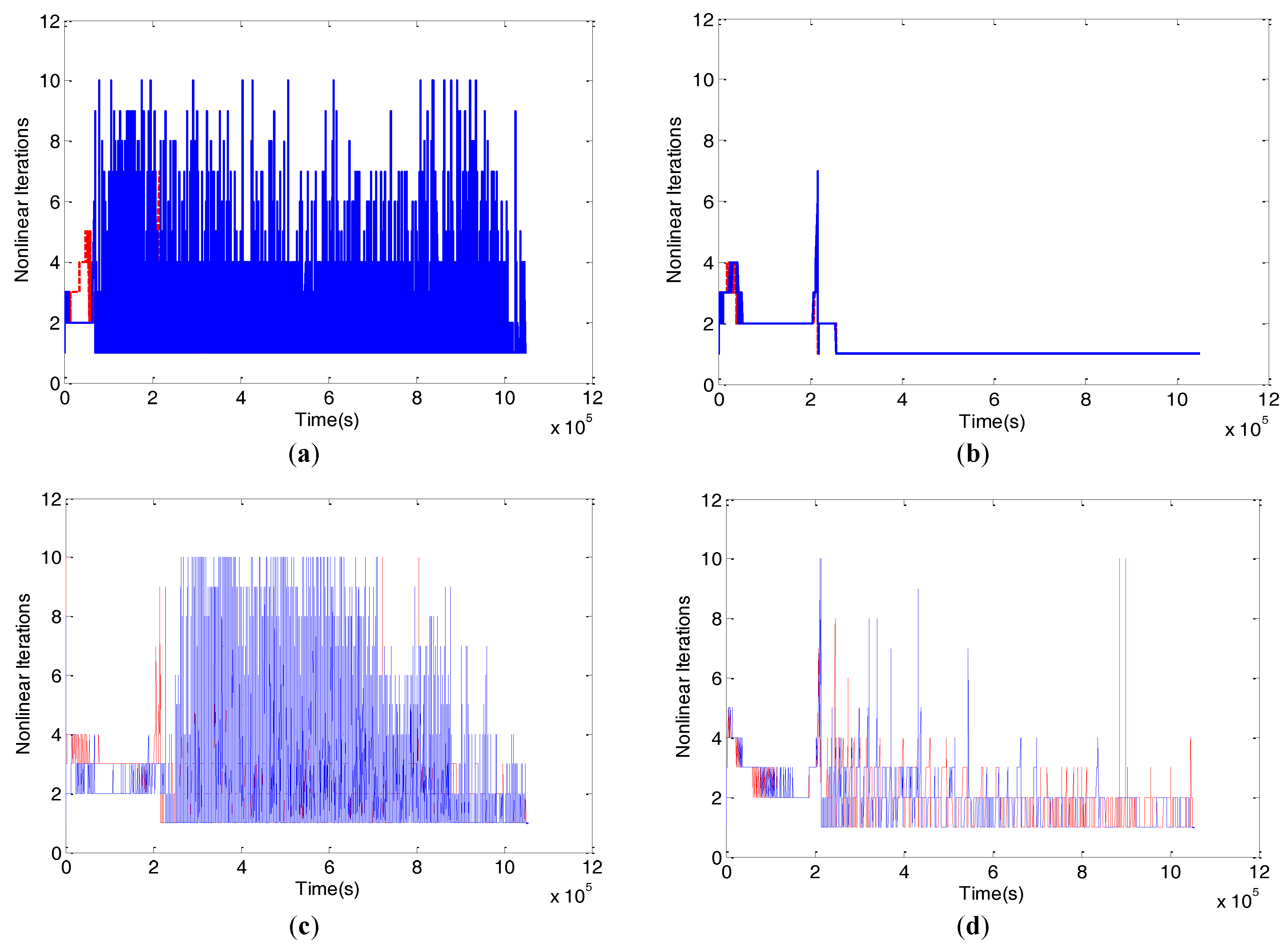
The time stepping, nonlinear convergence and cumulative mass balance error behavior for 150 layers with a step size of 1000 s of uniform and non-uniform NLKP are illustrated in Figure 5, Figure 6 and Figure 7, respectively. Graphs for the 150 layer simulation with 100 s and for the 50 layer cases are not presented here, but the observed results are discussed.
The graphical representation of time stepping (Figure 5) for NLKP = 31 shows that the non-uniform case never achieved the assigned maximum time step size of 1000 s for 150 layers except at the beginning and end time and that the uniform distribution shows the same behavior during the simulation period 1.0 × 10⁵ s to 2 × 10⁵ s. On the other hand, for NLKP = 151, both uniform and non-uniform cases of 150 layers achieved a maximum step size 1000 s. The performance of 50 layers with 31 lookup points is similar to 150 layers. Furthermore, it is found that the simulation is completed with the maximum step size 1000 s, except at the time near about 2 × 10⁵ s for 50 layers in the case of the uniform distribution.
For the Newton scheme, after 2.122 × 10⁵ s the uniform and non-uniform cases for all of the vertical layers with NLKP = 31 were unable to achieve the maximum step size 100 s throughout the simulation. Better performance is shown for the 1000 s case of 50 and 150 layers with NLKP = 31. For NLKP = 151, the time stepping behavior of the uniform and non-uniform cases is almost the same for both vertical discretizations.
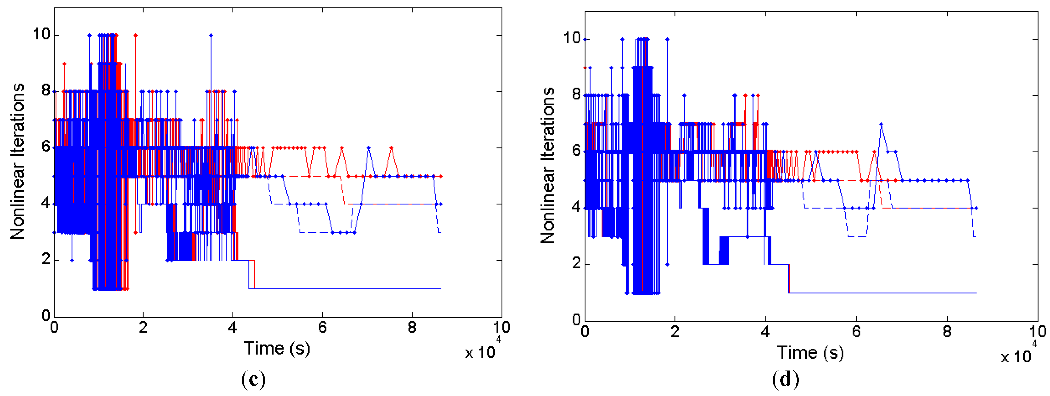
In Figure 6, the top two plots show the nonlinear iterations per time step of the Picard technique. Here, it is clear that the non-uniform distribution has difficulty meeting the convergence criterion for 150 layers with NLKP = 31 (similar results were obtained for 50 layers), whereas the uniform distribution needed only one iteration per time step for time step sizes of 1000 s. For 150 layers (as well as 50 layers) with NLKP = 151, both the uniform and non-uniform cases give almost the same behavior. The Newton scheme (bottom two plots of Figure 6) shows similar behaviors as we found in the Picard case. In this case, the uniform distribution of NLKP = 31 performs better than NLKP = 151.
Figure 7 shows the profiles of total volumetric mass balance error obtained from the uniform and non-uniform case of Picard and Newton techniques of 150 layers. The uniform distribution of NLKP = 31 and NLKP = 151 shows smaller errors for both the Picard and Newton schemes.
The comparison of the computational performance of the lookup table tests is summarized in Table 4 for the Picard and Newton schemes for the runs with and . Efficiency analysis of performance indicators for the Picard and Newton schemes is discussed as follows.
For the Picard scheme, the case of 50 layers, uniform distributions give better results for all criteria except CPU with for both sets (31 and 151) of lookup points; however, for the case (results not shown), the non-uniform distribution gives better results on the basis of mass balance error and linear iterations per nonlinear iteration, and for 150 layers of NLKP = 31 with the 100 s and 1000 s cases, the performance of uniform distribution is better than non-uniform on the basis of volumetric mass balance error. On the other hand, for 151 lookup points, the non-uniform case results are better than the uniform case for both time step sizes. For 50 layers and NLKP = 31, in terms of mass balance in percentage error, the uniform case performs better than the non-uniform for the 100 s time step size, but for the 1000 s case, the performance is reversed. Non-uniform performs better than uniform for both time step sizes with NLKP = 151. For the 150 layers case, the uniform distribution is the better strategy for all of the investigated cases (100 s and 1000 s and NLKP = 31 and 151). For both the 50 and 150 layer cases, when 100 s is considered, the uniform distribution takes fewer time steps for every set of NLKP. For 150 layers with NLKP = 31, the uniform case needs only 10,558 time steps to complete the simulation, whereas the non-uniform lookup distribution takes many more time steps (28,699). For both layer discretizations with NLKP = 151, the uniform and non-uniform cases take a comparable number of time steps for the time step size of 1000 s, but for the 31 lookup point case (with 100 s), uniform is much better than non-uniform. The uniform distribution is better at achieving the maximum time step size for 100 s for both vertical layers with 31 and 151 NLKP. For 1000 s and NLKP = 151, the non-uniform distribution case is better than the uniform distribution. On the overall assessment of this case, the uniform distribution points need fewer iterations to achieve convergence for all of the cases. The results show that the uniform distribution needs fewer linear iterations per nonlinear iteration to satisfy the termination criteria, except for the case of NLKP = 151 with 1000 s of 150 layers. Very little back stepping (only 17) occurs in the case of uniform distribution, but for the non-uniform case, this happened 6969 times for 150 layers with NLKP = 31. Thus, a back stepping assessment implies uniform distributions are preferable.
For the Newton scheme, the findings are: for the 100 s case, at 50 layers, the non-uniform distribution gives better results than the uniform distribution for NLKP = 31 for both cumulative mass balance error in and also in percentage, but completely opposite results are found for NLKP = 151. Uniform distributions of 150 layers clearly show superior performance for both NLKP with 100 s. For the 1000 s case, it is the non-uniform distributions that perform better. For the NLKP = 151 case, uniform is better than non-uniform for both grid discretizations, but for NLKP = 31, non-uniform takes fewer time steps than the uniform distribution for 100 s. Except for NLKP = 31 of 50 layers for the 1000 s case, uniform needs fewer time steps than non-uniform. The uniform distribution with 151 lookup points of both spatial discretizations achieved bigger average time step sizes for 100 s and 1000 s, but for 31 lookup points, the non-uniform case achieves a larger average time step size. For all of the cases, uniform distributions take fewer nonlinear iterations per time step to meet the convergence criterion. For the 50 layer case, non-uniform needs fewer linear iterations per nonlinear iteration to satisfy the termination criteria for all of the cases. For the 150 layers case, the uniform distribution leads to advanced performance except for NLKP = 151 with 100 s. For 50 layers, the uniform distribution of lookup points does more back stepping than the non-uniform case for NLKP = 31, but when NLKP = 151, it does less back stepping for both step sizes. For 150 layers with NLKP = 151, the uniform distribution does less back stepping than the non-uniform, but with 31 points, the opposite occurred. The number of solver failures is less for all of the cases of uniform distributions with 150 layers, but it is more for 50 layers.
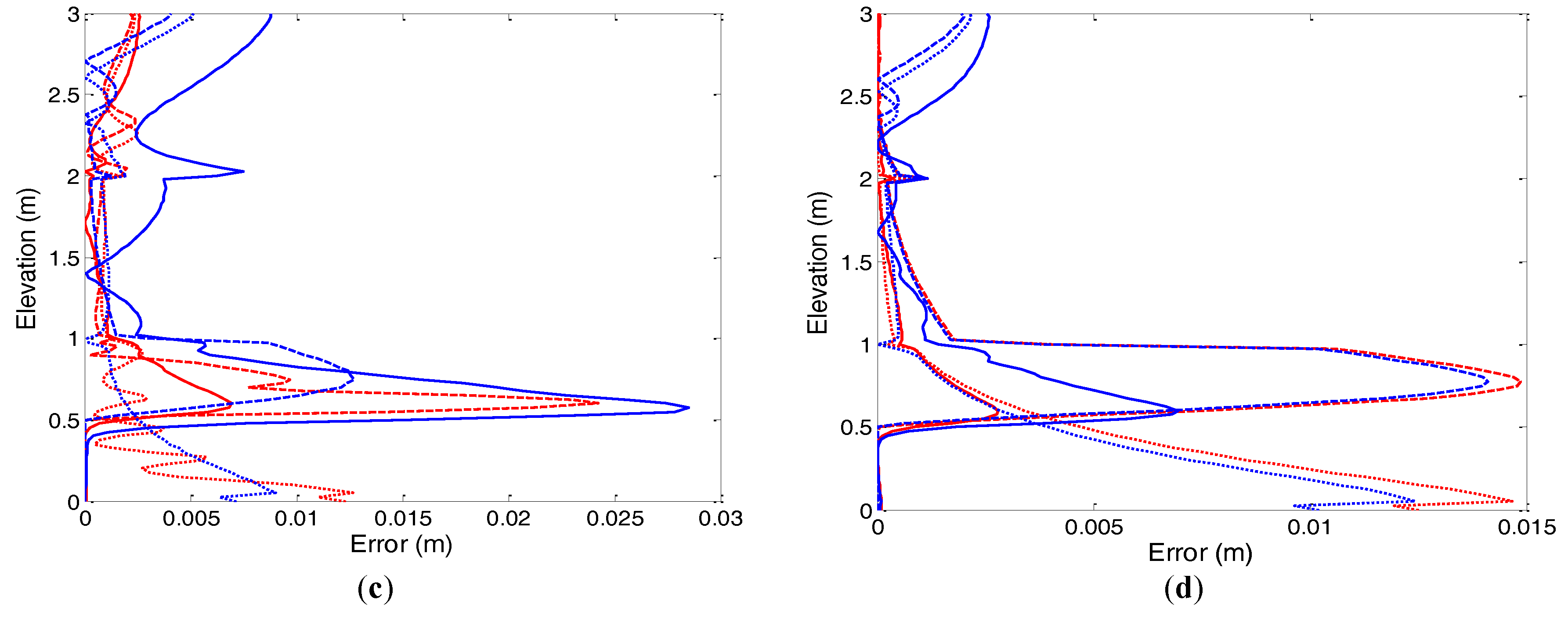
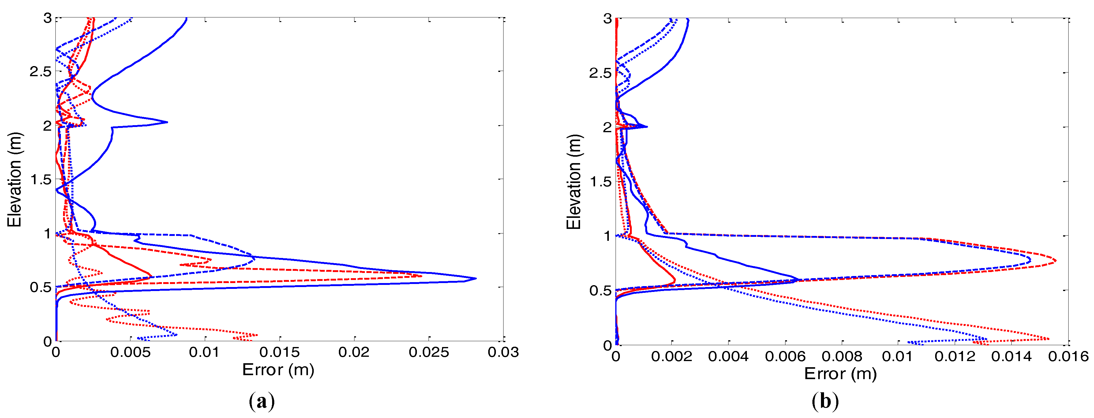
The root mean squared error (RMSE) behavior for the lookup tests under Picard and Newton iterations is shown in Figure 8 for the case 100 s, and the results are summarized in Table 5. The RMSEs are evaluated using the generated reference solution (301 nodes in the vertical soil column, 301 lookup points, step size 1 s and specified nonlinear tolerance 10−3. The results from these figures show that the uniform distribution scheme is as efficient as the non-uniform distribution method for all cases. Similar performance is observed for the step size of 1000 s of 50 and 150 layers.
4.3. Test Problem 3
The present test problem involves one-dimensional flow into an initially dry, 3 m deep, layered soil of sand and clay. The van Genuchten model is used to describe the soil moisture retention curves. The hydraulic properties of the sand and clay are given in Table 6, and the initial pressure head is set to −480 cm. The soil profile is sand for 0 < z < 100 cm and 200 cm < z < 300 cm and clay for 100 cm < z < 200 cm. A no-flow boundary condition is applied everywhere except for a water flux rate of 50 cm/day that is applied to the top of the vertical soil column, and the simulation period is one day. This problem was specifically devised for testing the numerical algorithm’s ability to survive both very dry conditions and transitions to a saturated state.
To explore the behavior of lookup table points for solving Richards’ equation, two levels of spatial grid sizes, (120 layers), three different time step sizes, 10 s, 800 s and 1600 s, and two sets of lookup points (31 and 151) in the soil moisture retention curves were used in the simulation. This kind of test problem is very complicated to simulate. The lookup points are concentrated in the sharp region of the moisture curves for the non-uniform distribution case. There are 24 runs in total for the iteration schemes (Picard and Newton).
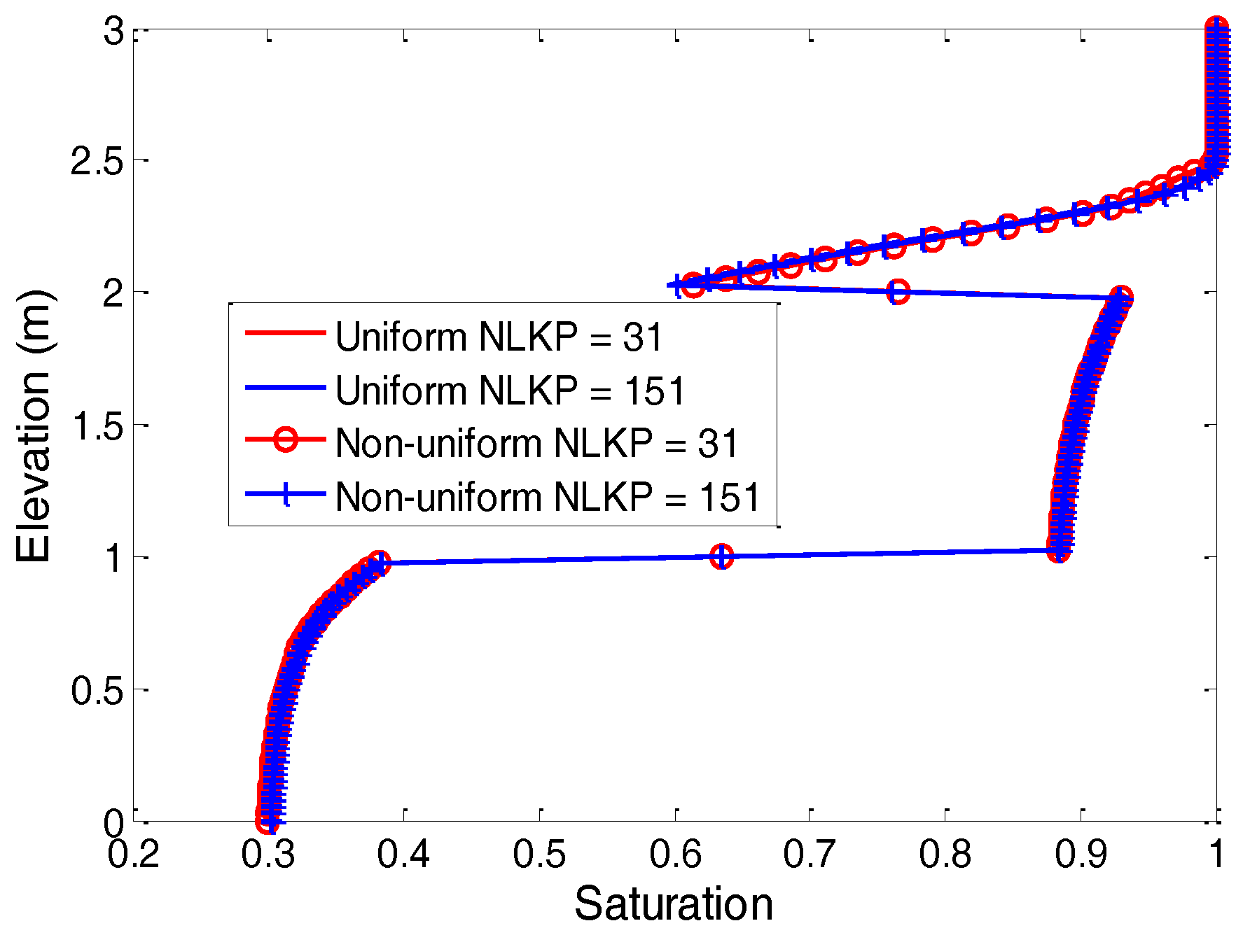
The van Genuchten soil moisture curves for the uniform and non-uniform distribution of lookup points are presented in Figure 9 and Figure 10. The computed water saturation after one day is illustrated in Figure 11 for all cases of uniform and non-uniform distribution strategies. All solutions obtained using both grid discretizations are in good agreement. Although numerical solutions to hydrological models are known to be quite sensitive to grid resolution [44,45,46], both of the grid sizes used in this test problem (60 layers and 120 layers) are sufficient to capture accurately the dynamics of this infiltration test case.
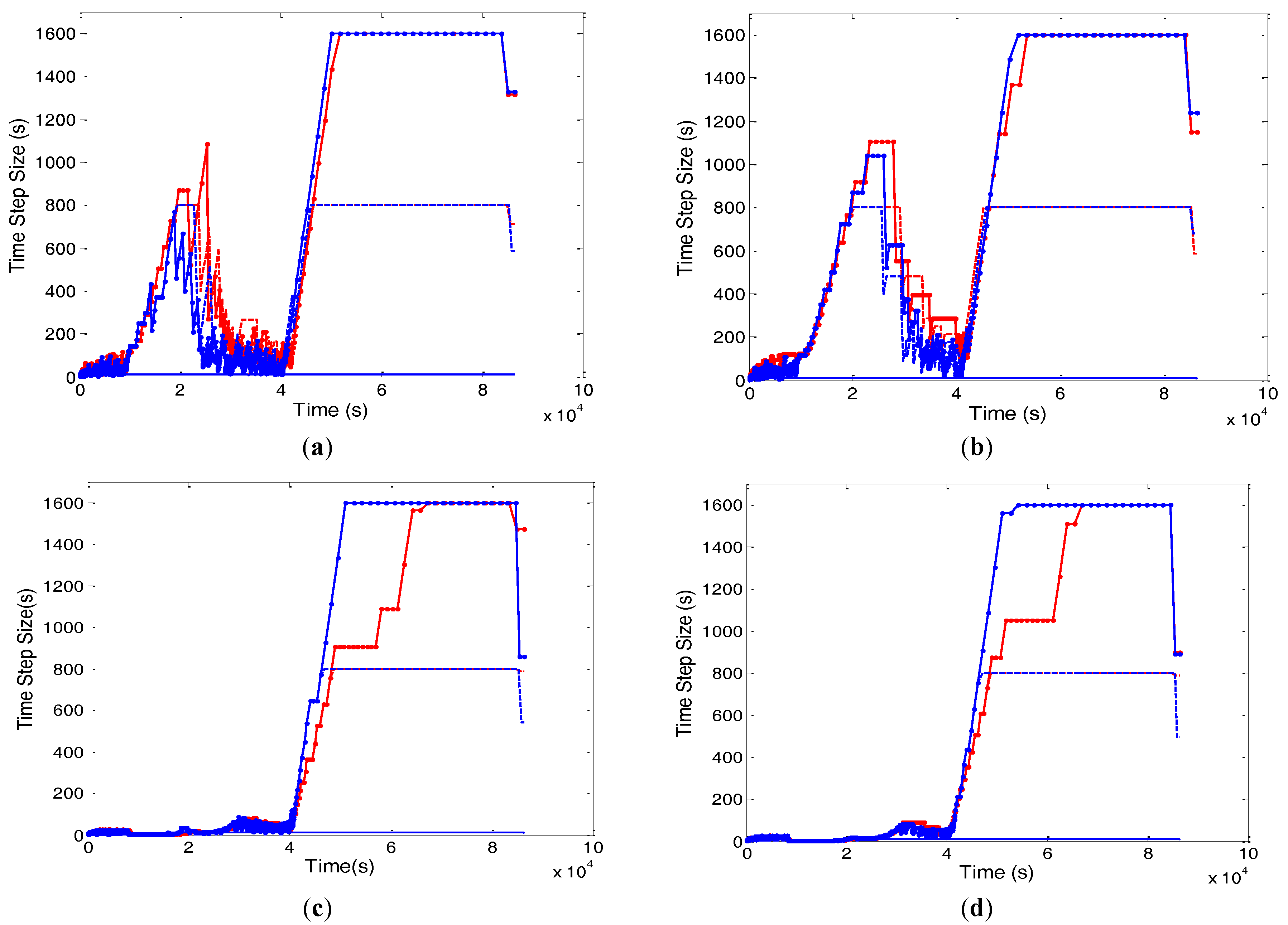
The time stepping, nonlinear convergence and cumulative mass balance error plots for the 120 layers case of uniform and non-uniform NLKP are presented in Figure 12, Figure 13 and Figure 14 for the Picard and Newton schemes. From the Picard time stepping graph (top two of Figure 12), the uniform distribution takes bigger time steps for the two sets of lookup points with 800 s and 1600 s from the beginning to 40,000 s, after which, there is little difference between the behavior of the uniform and non-uniform distributions. For 10 s, both the uniform and non-uniform cases run with the maximum step size until the end of the simulation. For the Newton case, after 40,000 s, the non-uniform case performs better for all runs with 1600 s. Before this time, the uniform and non-uniform cases behave comparably for all runs. The evolution of nonlinear Picard iterations (Figure 13) shows that the non-uniform case needs fewer iterations per time step compared to the uniform distribution of 800 s and 1600 s step sizes for each NLKP. Better performance is shown for the case of 10 s. On the other hand, converse results are obtained for the Newton run. The dissimilarity in performance of the two iterative schemes on account of convergence behavior is exhibited for this test problem compared to the previous problem. The cumulative mass balance error graphs for Picard and Newton (Figure 14) show that Picard performs better with uniformly-distributed lookup points, while Newton does better in the non-uniform case.
Table 7 summarizes the results of the lookup table tests of the numerical model for the Picard and Newton iterative schemes. The computational performances are discussed one by one for the Picard and Newton schemes as follows.
Non-uniform spatial discretizations in the retention curves give smaller volumetric mass balance errors for all layers and step sizes of the Picard iterative technique. According to the results in percentage mass balance error, the non-uniform case again performs better. For all combinations of NLKP and step sizes, the uniform allocation approach required a smaller number of time steps than the non-uniform case to complete the one-day simulation. On the basis of average time step size per time step, for all categories, the uniform distribution attained a larger value than the non-uniform case. Except for the time step size 1600 s case, non-uniform meshes needed fewer nonlinear iterations per time step to meet the convergence criteria. For each selection of NLKP with every time step size, less back stepping occurred for the uniform case.
For the Newton scheme, observations are: uniformly distributed lookup points produce smaller volumetric mass balance errors than the non-uniform case for 800 s and 1600 s and for both settings of NLKP and vertical layer discretization. On the other hand, for the 10 s time step size, very close values are obtained for the uniform and non-uniform approaches. On the basis of percentage error of volumetric mass balance outcomes, the same behavior is found for uniform and non-uniform cases, as we saw for total volumetric mass balance error. The uniform strategy needs many more time steps to complete the simulation for the cases of time step size 800 s and 1600 s for 120 layers. For NLKP = 31 of 60 layers, the average time step for uniform distributions is larger than for non-uniform in the case of 10 s and 800 s, but for the 1600 s, the non-uniform case is larger. In the case of NLKP = 31 of 120 layers, the non-uniform achieves bigger step sizes for 10 s and 800 s, but not for the 1600 s case. For NLKP = 151 of 120 layers, in the 800 s and 1600 s cases, uniform distributions perform better, but not for the 10 s case. For the 60 layers case, the non-uniform distribution takes fewer nonlinear iterations per time step except for the 1600 s case. In the case of 10 s with NLKP = 151 of 120 layers, the uniform and non-uniform runs achieve a very close value of nonlinear iterations per time step (4.06 and 4.07, respectively). Fewer back steps occur for all of the uniform distribution cases compared to the non-uniform distribution of lookup points. There is little difference between uniform and non-uniform distributions in terms of linear solver failures.
The RMSE performance for uniform and non-uniform distributions of lookup points is shown in Figure 15 for the Picard (top two) and Newton (bottom two) schemes. The numerically-generated reference solution is made with a dense grid, (240 layers), NLKP = 301, time step size is 1 s, convergence tolerance of . The comparison of calculated RMSE at three different times (32,000 s, 56,000 s and 86,400 s) for both cases are presented in Table 8. For the Picard method, for NLKP = 31 with 10 s, the uniform case shows smaller error only at time 32,000 s, while at times 56,000 s and 86,400 s, the non-uniform case performs better. Note that, for 800 s and 1600 s, the non-uniform case gives smaller values than the uniform case for both layers, except at time 56,000 s. For NLKP = 151 and 60 layers, the uniform case shows smaller root mean squared errors than non-uniform, but for 120 layers, the values are same at the three time levels for 10 s. For 800 s and 1600 s, the non-uniform distribution performs better for each of the layers at the three indicated simulation time levels. For the Newton iterative scheme, we found that the RMSE values at the three different times for the uniform distribution are smaller than for the non-uniform distribution for all cases except 10 s.
5. Conclusions
We have shown that the lookup table method for evaluating the soil moisture retention curves in Richards’ equation-based models is an accurate and efficient alternative to analytical evaluation that can be useful for dealing with heterogeneous problems. The comparative performance between the uniform and non-uniform distribution options for the lookup table points depends on the indicators being examined. If we focus on the number of time steps, average time step size, nonlinear iterations per time step, linear iterations per nonlinear iteration, back stepping and solver failures, we can say that the uniform distribution is the better strategy. In terms of total volumetric and percentage mass balance errors, the two options give similar results. In terms of the RMSE, the uniform option again appears to have an edge over the non-uniform choice. For other configurations of layers, NLKP and other parameters, the relative performances vary, and it is difficult to draw a general conclusion concerning the best choice between the uniform and non-uniform distributions.
The objectives of our modeling included the development and implementation of a numerical procedure for the effective simulation of flow through porous media under variably-saturated conditions within complex geometries, using uniform and non-uniform distributions of lookup table points for evaluating the soil hydraulic characteristics and the derivatives of these strongly nonlinear relationships. This contribution describes the implementation, testing and evaluation of an effective procedure for the simulation of variably-saturated flow in porous media with spatially-varying properties, e.g., by taking many points in the sharp region of soil moisture curves. We have solved accurately and with high computational efficiency some discriminating tests cases involving relatively extreme conditions with regard to vertical drainage through a layered soil from initially-saturated conditions and sharp boundaries between the unsaturated and saturated conditions. The various factors affecting the performance of the Picard and Newton schemes are illustrated and summarized for two test cases and numerous combinations of grid size, time step size and number of lookup points. We have shown that the uniform distribution is the better strategy to solve Richards’ equation for drainage problems, while the non-uniform discretizations can be chosen for layered soil problems. Further research will investigate 2D and 3D flow domains.
Acknowledgments
This work was made possible by the support provided by the EMMA and the Department of Mathematics, University of Padova, Italy. We thank the reviewers for their detailed and very helpful comments. There are no funds to cover any costs for openaccess.
Author Contributions
The work described in this paper was performed by the first author as part of his PhD research, supervised by the second and third authors. All authors contributed to the conceptualization and writing of this paper, with the first version prepared by the first author.
Conflicts of Interest
The authors declare no conflict of interest.
References
- Arampatzis, G.; Tzimopoulos, C.; Sakellariou-Makrantonaki, M.; Yannopoulos, S. Estimation of unsaturated flow in layered soils with the finite control volume method. Irrig. Drain 2001, 50, 349–358. [Google Scholar] [CrossRef]
- Koorevaar, P.; Menelik, G.; Dirksen, C. Elements of Soil Physics; Developments in Soil Science 13; Elsevier Science Publishers B.V.: Amsterdam, The Netherlands, 1983; p. 228. [Google Scholar]
- Miller, C.T.; Abhishek, C.; Farthing, M.W. A spatially and temporally adaptive solution of Richards’ equation. Adv. Water Resour. 2005, 29, 525–545. [Google Scholar] [CrossRef]
- Celia, M.A.; Bouloutas, E.T.; Zarba, R.L. A General mass-conservative numerical solution for the unsaturated flow equation. Water Resour. Res. 1990, 26, 1483–1496. [Google Scholar] [CrossRef]
- Celia, M.A.; Binning, P. A mass conservative numerical solution for two-phase flow in porous media with application to unsaturated flow. Water Resour. Res. 1992, 28, 281–928. [Google Scholar] [CrossRef]
- Miller, C.T.; Williams, G.A.; Kelly, C.T.; Tocci, M.D. Robust solution of Richards’ equation for nonuniform porous media. Water Resour. Res. 1998, 34, 2599–2610. [Google Scholar] [CrossRef]
- Ogden, F.L.; Lai, W.; Steinke, R.C.; Zhu, J.; Talbot, C.A.; Wilson, J.L. A new general 1-D vadose zone flow solution method. Water Resour. Res. 2015, 51, 4282–4300. [Google Scholar] [CrossRef]
- Tocci, M.D.; Kelley, C.T.; Miller, C.T. Accurate and economical solution of the pressure-head form of Richards’ equation by the method of lines. Adv. Water Resour. 1997, 20, 1–14. [Google Scholar] [CrossRef]
- Vogel, T.; van Genuchten, M.T.; Cislerova, M. Effect of the shape of the soil hydraulic functions near saturation on variably-saturated flow predictions. Adv. Water Resour. 2001, 24, 133–144. [Google Scholar] [CrossRef]
- Diersch, H.J.G.; Perrochet, P. On the primary variable switching technique for simulating unsaturated-saturated flows. Adv. Water Resour. 1999, 23, 271–301. [Google Scholar] [CrossRef]
- Forsyth, P.A.; Wu, Y.S.; Pruess, K. Robust numerical methods for saturated-unsaturated flow with dry initial conditions in heterogeneous media. Adv. Water Resour. 1995, 18, 25–38. [Google Scholar] [CrossRef]
- Kirkland, M.R.; Hills, R.G.; Wierenga, P.J. Algorithms for solving Richards’ equation for variably saturated soils. Water Resour. Res. 1992, 28, 2049–2058. [Google Scholar] [CrossRef]
- Huang, K.; Mohanty, B.; van Genuchten, M.M. A new convergence criterion for the modified iteration method for solving the variably saturated flow equation. J. Hydrol. 1996, 178, 69–91. [Google Scholar] [CrossRef]
- Hills, R.; Hudson, I.; Wierenga, P. Modeling one-dimensional infiltration into very dry soils: 1. Model development and evaluation. Water Resour. Res. 1989, 25, 1271–1282. [Google Scholar] [CrossRef]
- Matthews, C.J.; Braddock, R.D.; Sander, G. Modeling flow through a one-dimensional multi-layered soil profile using the Method of Lines. Environ. Model Assess. 2004, 9, 103–113. [Google Scholar] [CrossRef]
- Schiesser, W.E. The Numerical Method of Lines: Integration of Partial Differential Equations; Academic Press: San Diego, CA, USA, 1991. [Google Scholar]
- D’Haese, C.M.F.; Putti, M.; Paniconi, C.; Verhoest, N.E.C. Assessment of adaptive and heuristic time stepping for variably saturated flow. Int. J. Numer. Methods Fluids 2007, 53, 1173–1193. [Google Scholar] [CrossRef]
- Bergamaschi, L.; Putti, M. Mixed finite elements and Newton-type linearizations for the solution of Richards’ equation. Int. J. Numer. Methods Eng. 1999, 45, 1025–1046. [Google Scholar] [CrossRef]
- Paniconi, C.; Putti, M. A comparison of Picard and Newton iteration in the numerical solution of multidimensional variably saturated flow problems. Water Resour. Res. 1994, 30, 3357–3374. [Google Scholar] [CrossRef]
- Clement, T.P.; William, R.W.; Molz, F.J. A physically based two-dimensional, finite difference algorithm for modeling variably saturated flow. J. Hydrol. 1994, 161, 71–90. [Google Scholar] [CrossRef]
- Jones, J.E.; Woodward, C.S. Newton-krylov-Multigrid solvers for large-scale, highly heterogeneous, variably saturated flow problems. Adv. Water Resour. 2001, 24, 763–774. [Google Scholar] [CrossRef]
- Manzini, G.; Ferraris, S. Mass-conservative finite volume methods in 2-D unsaturated grid for the Richards equation. Adv. Water Resour. 2004, 27, 1199–1215. [Google Scholar] [CrossRef]
- Simunek, J.; Sejna, M.; van Genuchten, M.T. HYDRUS-2D: Simulating Water Flow and Solute Transport in Two-Dimensional Variably Saturated Media; Technology Research; IGWMC Golden: CO, USA, 1999. [Google Scholar]
- Abriola, L.M.; Lang, J.R. Self-adaptive finite element solution of the one dimensional unsaturated flow equation. Int. J. Numer. Methods Fluids 1990, 10, 227–246. [Google Scholar] [CrossRef]
- Ju, S.H.; Kung, K.J.S. Mass types, Element orders and Solution schemes for Richards’ equation. Comput. Geosci. 1997, 23, 175–187. [Google Scholar] [CrossRef]
- Milly, P.C.D. A mass-conservative procedure for time-stepping in models of unsaturated flow. Adv. Water Resour. 1985, 8, 32–36. [Google Scholar] [CrossRef]
- Kavetski, D.; Binning, P.; Sloan, S.W. Noniterative time stepping schemes with adaptive truncation error control for the solution of Richards’ equation. Water Resour. Res. 2002, 38, 1211–1220. [Google Scholar] [CrossRef]
- Paniconi, C.; Aldama, A.A.; Wood, E.F. Numerical evaluation of iterative and noniterative methods for the solution of the nonlinear Richards’ equation. Water Resour. Res. 1991, 27, 1147–1163. [Google Scholar] [CrossRef]
- Cooley, R.L. Some new procedures for numerical solution of variably saturated flow problems. Water Resour. Res. 1983, 19, 1271–1285. [Google Scholar] [CrossRef]
- Culham, W.E.; Varga, R.S. Numerical methods for time-dependent, nonlinear boundary value problems. Soc. Pet. Eng. J. 1971, 11, 374–388. [Google Scholar] [CrossRef]
- Faust, C.R. Transport of immiscible fluids within and below the unsaturated zone: A numerical model. Water Resour. Res. 1985, 21, 587–596. [Google Scholar] [CrossRef]
- Huyakorn, P.S.; Thomas, S.D.; Thompson, B.M. Techniques for making finite elements competitive in modeling flow in variably saturated media. Water Resour. Res. 1984, 20, 1099–1115. [Google Scholar] [CrossRef]
- Huyakorn, P.S.; Jones, B.G.; Andersen, P.F. Finite element algorithms for simulating three-dimensional groundwater flow and solute transport in multilayer systems. Water Resour. Res. 1986, 23, 361–374. [Google Scholar] [CrossRef]
- Huyakorn, P.S.; Springer, E.P.; Guvanasen, V.; Wadsworth, T.D. A three dimensional finite element model for simulating water flow in variably saturated porous media. Water Resour.Res. 1986, 22, 1790–1808. [Google Scholar] [CrossRef]
- Ross, P.J. Efficient numerical methods for infiltration using Richards’ equation. Water Resour. Res. 1990, 26, 279–290. [Google Scholar] [CrossRef]
- Baca, R.G.; Chung, J.N.; Mulla, D.J. Mixed transform finite element method for solving the non-linear equation for flow in variably saturated porous media. Int. J. Numer. Methods. Fluids 1997, 24, 441–445. [Google Scholar] [CrossRef]
- Guarracino, L.; Quintana, F. A third-order accurate time scheme for variably saturated groundwater flow modeling. Commun. Numer. Methods Eng. 2004, 20, 379–389. [Google Scholar] [CrossRef]
- Brooks, R.H.; Corey, A.T. Properties of porous media affecting fluid flow. J. Irrig. Drain. Div. Am. Soc. Civ. Eng. 1966, 92, 61–88. [Google Scholar]
- Van Genuchten, M.T. A Closed-form Equation for Predicting the Hydraulic Conductivity of Unsaturated Soils. Soil Sci. Soc. Am. J. 1980, 44, 892–898. [Google Scholar] [CrossRef]
- Camporese, M.; Paniconi, C.; Putti, M.; Orlandini, S. Surface-subsurface flow modeling with path-based runoff routing, boundary condition-based coupling, and assimilation of multisource observation data. Water Resour. Res. 2010, 46, W02512. [Google Scholar] [CrossRef]
- Casulli, V.; Zanolli, P. A nested Newton-type algorithm for finite volume methods solving Richards’ equation in mixed form. SIAM J. Sci. Comput. 2010, 32, 2255–2273. [Google Scholar] [CrossRef]
- Marinelli, F.; Durnford, D.S. Semi analytical solution to Richards’ equation for layered porous media. J. Irrig. Drain. Eng. 1998, 124, 290–299. [Google Scholar] [CrossRef]
- McBride, D.; Cross, M.; Croft, N.; Bennett, C.; Gebhardt, J. Computational modeling of variably saturated flow in porous media with complex three-dimensional geometries. Int. J. Numer. Methods Fluids 2006, 50, 1085–1117. [Google Scholar] [CrossRef]
- Kuo, W.L.; Steenhuis, T.S.; McCulloch, C.E.; Mohler, C.L.; Weinstein, D.A.; DeGloria, S.D.; Swaney, D.P. Effect of grid size on runoff and soil moisture for a variable-source-area hydrology model. Water Resour. Res. 1999, 35, 3419–3428. [Google Scholar] [CrossRef]
- Son, K.; Tague, C.; Hunsaker, C. Effects of model spatial resolution on ecohydrologic predictions and their sensitivity to inter-annual climate variability. Water 2016, 8, 321. [Google Scholar] [CrossRef]
- Sulis, M.; Paniconi, C.; Camporese, M. Impact of grid resolution on the integrated and distributed response of a coupled surface–subsurface hydrological model for the des Anglais catchment, Quebec. Hydrol. Process. 2011, 25, 1853–1865. [Google Scholar] [CrossRef]
Figure 1.
Saturation profiles for Test Problem 1 at four different times for the analytical method (red) and for the lookup table method with 31 (blue) and 151 (green) lookup points distributed uniformly.
Figure 1.
Saturation profiles for Test Problem 1 at four different times for the analytical method (red) and for the lookup table method with 31 (blue) and 151 (green) lookup points distributed uniformly.

Figure 2.
Soil moisture curves for the uniform and non-uniform lookup table points of Soil 1.

Figure 3.
Soil moisture curves for the uniform and non-uniform lookup table points of Soil 2.
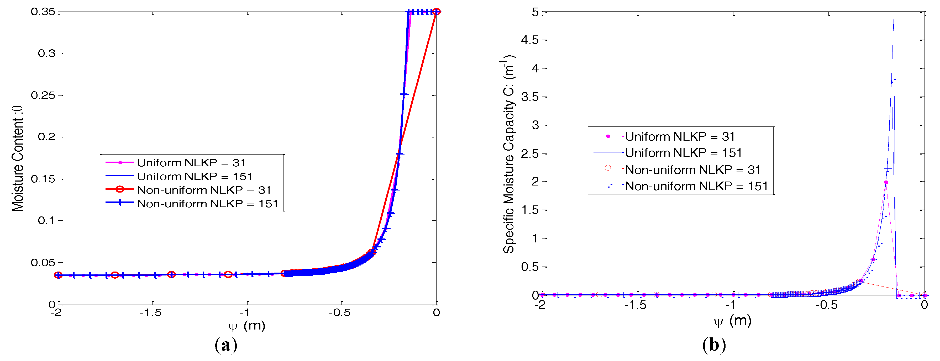
Figure 4.
Saturation predictions after 12.15 days for the uniform and non-uniform lookup table point cases, Picard scheme.
Figure 4.
Saturation predictions after 12.15 days for the uniform and non-uniform lookup table point cases, Picard scheme.

Figure 5.
Comparison of time stepping behavior of Picard (a,b) and Newton (c,d) scheme of uniform (red) and non-uniform (blue) of 31 (a,c) and 151 (b,d) lookup points for 150 layers.
Figure 5.
Comparison of time stepping behavior of Picard (a,b) and Newton (c,d) scheme of uniform (red) and non-uniform (blue) of 31 (a,c) and 151 (b,d) lookup points for 150 layers.


Figure 6.
Comparison of convergence behavior of Picard (a,b) and Newton (c,d) scheme of uniform (red) and non-uniform (blue) of 31 (a,c) and 151 (b,d) lookup points for 150 layers.
Figure 6.
Comparison of convergence behavior of Picard (a,b) and Newton (c,d) scheme of uniform (red) and non-uniform (blue) of 31 (a,c) and 151 (b,d) lookup points for 150 layers.

Figure 7.
Comparison of cumulative mass balance behavior of Picard (a,b) and Newton (c,d) scheme of uniform (red) and non-uniform (blue) of 31 (a,c) and 151 (b,d) lookup points for 150 layers.
Figure 7.
Comparison of cumulative mass balance behavior of Picard (a,b) and Newton (c,d) scheme of uniform (red) and non-uniform (blue) of 31 (a,c) and 151 (b,d) lookup points for 150 layers.
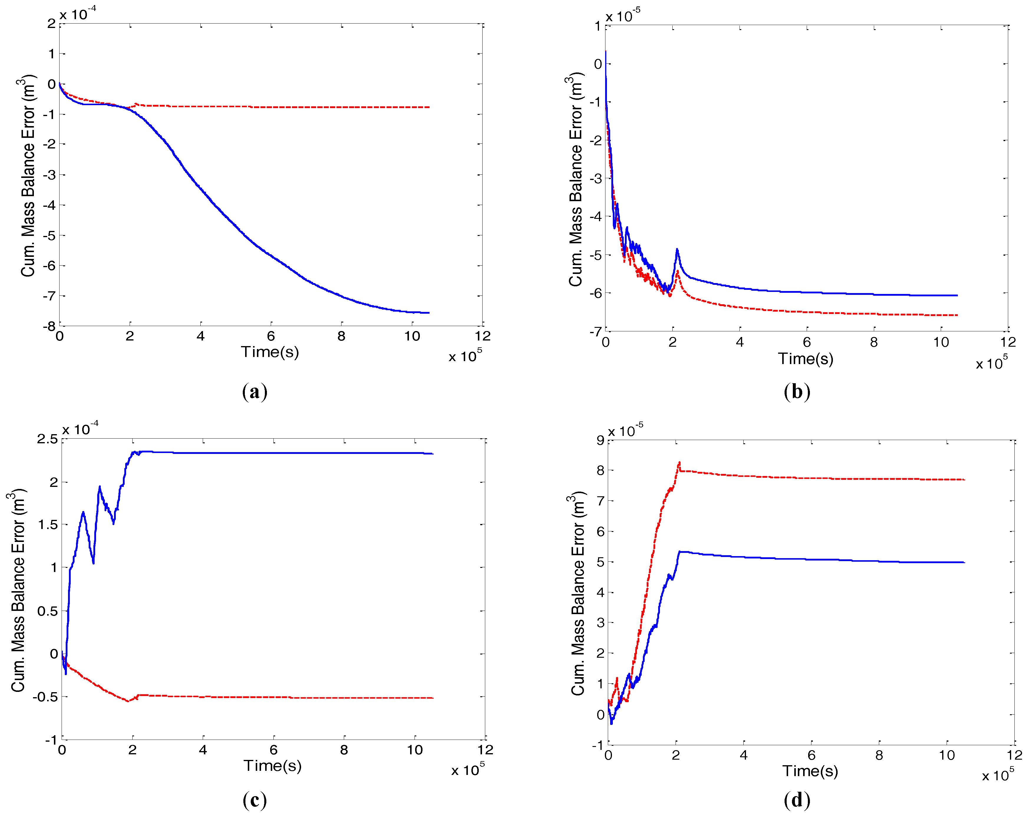
Figure 8.
Computed RMSE for Picard (a,b) and Newton (c,d) schemes for the uniform (red) and non-uniform (blue) NLKP = 31 (a,c) and NLKP = 151 (b,d) lookup point cases for 150 layers. RMSE is calculated at 250,000 s (solid), 550,000 s (dotted) and 1,050,000 s (dashed).
Figure 8.
Computed RMSE for Picard (a,b) and Newton (c,d) schemes for the uniform (red) and non-uniform (blue) NLKP = 31 (a,c) and NLKP = 151 (b,d) lookup point cases for 150 layers. RMSE is calculated at 250,000 s (solid), 550,000 s (dotted) and 1,050,000 s (dashed).
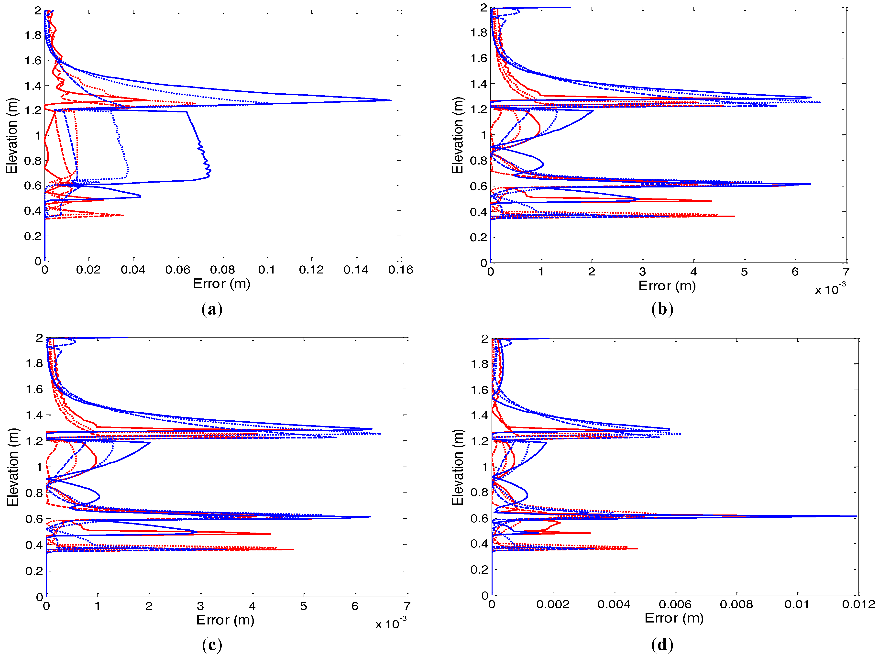
Figure 9.
Sandy soil moisture curves for the uniform and non-uniform lookup table point cases.
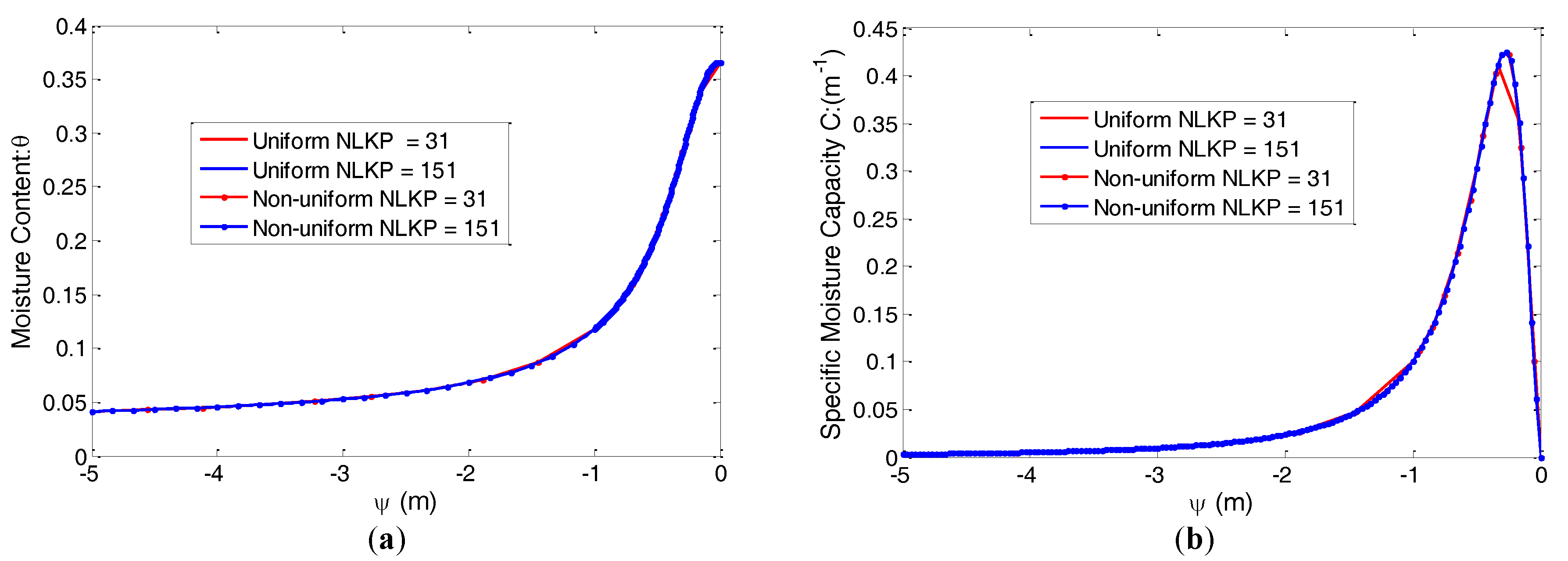
Figure 10.
Clay soil moisture curves for the uniform and non-uniform lookup table point cases.

Figure 11.
Computed water saturation after 1 day for uniform and non-uniform lookup points.

Figure 12.
Comparison of time stepping behavior of Picard (a,b) and Newton (c,d) scheme of uniform (red) and non-uniform (blue) of 31 (a,c) and 151 (b,d) lookup points of 120 layers for the step size 10 s (solid), 800 s (dashed) and 1600 s (dot-dashed).
Figure 12.
Comparison of time stepping behavior of Picard (a,b) and Newton (c,d) scheme of uniform (red) and non-uniform (blue) of 31 (a,c) and 151 (b,d) lookup points of 120 layers for the step size 10 s (solid), 800 s (dashed) and 1600 s (dot-dashed).

Figure 13.
Comparison of convergence behavior of Picard (a,b) and Newton (c,d) scheme of uniform (red) and non-uniform (blue) of 31 (a,c) and 151 (b,d) lookup points of 120 layers for the step size 10 s (solid), 800 s (dashed) and 1600 s (dot-dashed).
Figure 13.
Comparison of convergence behavior of Picard (a,b) and Newton (c,d) scheme of uniform (red) and non-uniform (blue) of 31 (a,c) and 151 (b,d) lookup points of 120 layers for the step size 10 s (solid), 800 s (dashed) and 1600 s (dot-dashed).
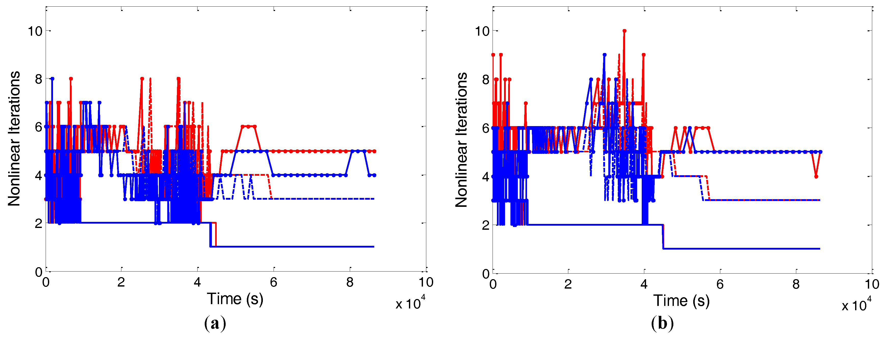

Figure 14.
Comparison of cumulative mass balance behavior for Picard (a,b) and Newton (c,d) scheme of uniform (red) and non-uniform (blue) of 31 (a,c) and 151 (b,d) lookup points of 120 layers for the step size 10 s (solid), 800 s (dashed) and 1600 s (dot-dashed).
Figure 14.
Comparison of cumulative mass balance behavior for Picard (a,b) and Newton (c,d) scheme of uniform (red) and non-uniform (blue) of 31 (a,c) and 151 (b,d) lookup points of 120 layers for the step size 10 s (solid), 800 s (dashed) and 1600 s (dot-dashed).
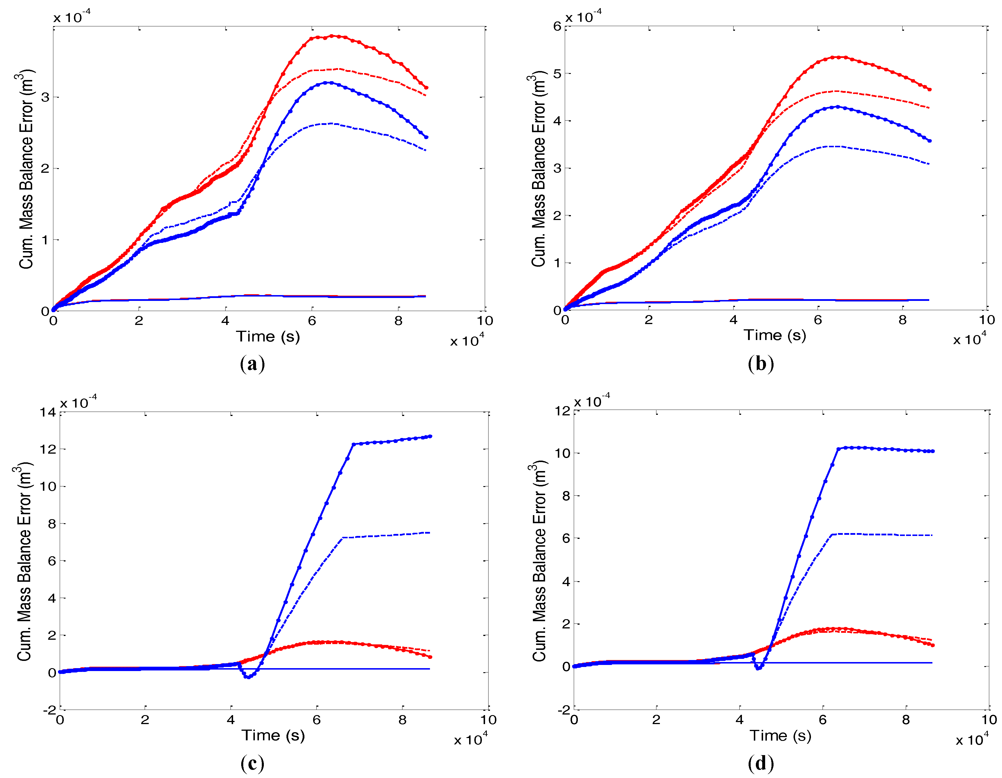
Figure 15.
Computed RMSE for Picard (a,b) and Newton (c,d) schemes for the uniform (red) and non-uniform (blue) NLKP = 31 (a,c) and NLKP = 151 (b,d) lookup point cases for 120 layers and step size 10 s. RMSE is calculated at 32,000 s (solid), 56,000 s (dashed) and 86,400 s (dot-dashed).
Figure 15.
Computed RMSE for Picard (a,b) and Newton (c,d) schemes for the uniform (red) and non-uniform (blue) NLKP = 31 (a,c) and NLKP = 151 (b,d) lookup point cases for 120 layers and step size 10 s. RMSE is calculated at 32,000 s (solid), 56,000 s (dashed) and 86,400 s (dot-dashed).


Table 1.
Soil hydraulic properties used in Test Problem 1.
| Parameters | Soil 1 | Soil 2 |
|---|---|---|
| 0.35 | 0.35 | |
| 0.07 | 0.07 | |
| 0.0286 | 0.0286 | |
| 1.5 | 1.5 | |
| 9.81 × 10⁻5 | 9.81 × 10⁻3 |
Table 2.
Performance of the lookup table and analytical methods for Test Problem 1.
| Performance criterion | No. of Layers | NLKP | s | s | ||||
|---|---|---|---|---|---|---|---|---|
| Lookup Table | Analytical | Lookup Table | Analytical | |||||
| Uniform | Non-Uniform | Uniform | Non-Uniform | |||||
| No. of time steps | 50 | 31 | 10,598 | 10,595 | 10,600 | 1167 | 1170 | 1182 |
| 151 | 10,594 | 10,594 | 1165 | 1175 | ||||
| 150 | 31 | 10,689 | 10,704 | 10,800 | 1323 | 1282 | 1402 | |
| 151 | 10,690 | 10,699 | 1300 | 1273 | ||||
| Mass balance error ( | 50 | 31 | −6.23 × 10⁻⁶ | −6.72 × 10⁻⁶ | −5.05 × 10⁻⁶ | −4.86 × 10⁻⁵ | −6.01 × 10⁻⁵ | −5.84 × 10⁻⁵ |
| 151 | −8.31 × 10⁻⁶ | −8.05 × 10⁻⁶ | −6.21 × 10⁻⁵ | −6.38 × 10⁻⁵ | ||||
| 150 | 31 | −5.24 × 10⁻⁶ | −5.93 × 10⁻⁶ | −8.61× 10⁻⁶ | −4.24 × 10⁻⁵ | −468 × 10−5 | −5.47 × 10⁻⁵ | |
| 151 | −8.25 × 10⁻⁶ | −7.72 × 10⁻⁶ | −4.72 × 10⁻⁵ | −4.79 × 10⁻⁵ | ||||
| CPU (s) | 50 | 31 | 449.01 | 438.01 | 536.82 | 77.75 | 74.76 | 86.34 |
| 151 | 816.03 | 830.10 | 125.15 | 132.36 | ||||
| 150 | 31 | 1661.33 | 1550.83 | 1779.71 | 425.87 | 396.35 | 496.56 | |
| 151 | 2686.82 | 2731.21 | 666.32 | 656.91 | ||||
Table 3.
Soil hydraulic properties used in Test Problem 2.
| Parameters | Soil 1 | Soil 2 |
|---|---|---|
| 0.35 | 0.35 | |
| 0.07 | 0.035 | |
| 0.0286 | 0.0667 | |
| 1.5 | 3.0 | |
| 9.81 × 10⁻⁵ | 9.81 × 10⁻³ |
Table 4.
Computational performance of the lookup table method for uniform and non-uniform cases of Picard and Newton iteration with discretizations of 50 and 150 layers and .
Table 4.
Computational performance of the lookup table method for uniform and non-uniform cases of Picard and Newton iteration with discretizations of 50 and 150 layers and .
| Performance criterion | No. of Layers | NLKP | Picard | Newton | ||
|---|---|---|---|---|---|---|
| Uniform | Non-uniform | Uniform | Non-uniform | |||
| Mass balance error ( | 50 | 31 | 5.01 × 10⁻⁶ | −1.13 × 10⁻⁵ | 8.15 × 10⁻⁶ | 6.60 × 10⁻⁶ |
| 151 | 8.03 × 10⁻⁶ | 7.51 × 10⁻⁵ | 9.59 × 10⁻⁶ | 9.73 × 10⁻⁶ | ||
| 150 | 31 | 3.34 × 10⁻⁶ | −6.69 × 10⁻⁴ | 6.71 × 10⁻⁶ | −1.35 × 10⁻⁵ | |
| 151 | 5.28 × 10⁻⁶ | 5.06 × 10⁻⁶ | 8.26 × 10⁻⁶ | 9.00 × 10⁻⁶ | ||
| Relative mass balance error (%) | 50 | 31 | −3.98 × 10⁻² | 8.93 × 10⁻² | 6.47 × 10⁻² | −5.12 × 10⁻² |
| 151 | −6.56 × 10⁻² | −6.04 × 10⁻² | −7.72 × 10⁻² | −7.84 × 10⁻² | ||
| 150 | 31 | −1.28 × 10⁻² | 5.04 × 100 | −5.33 × 10⁻² | 1.07 × 10⁻¹ | |
| 151 | −1.38 × 10⁻² | −4.07 × 10⁻² | −6.65 × 10⁻² | −7.25 × 10⁻² | ||
| No. of time steps | 50 | 31 | 10,567 | 10,583 | 35,081 | 14,074 |
| 151 | 10,566 | 10,584 | 29,024 | 29,993 | ||
| 150 | 31 | 10,558 | 28,699 | 85,175 | 61,544 | |
| 151 | 10,562 | 10,573 | 79,014 | 84,283 | ||
| Avg. (s) | 50 | 31 | 99.37 | 87.10 | 2.9.93 | 74.61 |
| 151 | 99.38 | 89.56 | 36.18 | 35.08 | ||
| 150 | 31 | 99.45 | 36.59 | 12.33 | 17.06 | |
| 151 | 99.41 | 99.31 | 13.29 | 12.46 | ||
| NL. iter/time step | 50 | 31 | 1.03 | 1.49 | 3.24 | 2.98 |
| 151 | 1.04 | 1.04 | 3.05 | 3.08 | ||
| 150 | 31 | 1.03 | 4.00 | 3.39 | 3.82 | |
| 151 | 1.03 | 1.03 | 3.38 | 3.39 | ||
| Lin. iter/NL. iter | 50 | 31 | 7.73 | 6.86 | 24.57 | 17.74 |
| 151 | 7.77 | 7.76 | 24.46 | 22.20 | ||
| 150 | 31 | 7.55 | 3.97 | 15.52 | 32.90 | |
| 151 | 7.60 | 7.57 | 15.18 | 14.15 | ||
| No. of back steps | 50 | 31 | 19 | 27 | 7898 | 1290 |
| 151 | 20 | 25 | 5972 | 6226 | ||
| 150 | 31 | 17 | 6969 | 20,245 | 13,863 | |
| 151 | 19 | 22 | 18,698 | 20,093 | ||
| Solver failures | 50 | 31 | 0 | 0 | 0 | 0 |
| 151 | 0 | 0 | 0 | 0 | ||
| 150 | 31 | 0 | 0 | 0 | 0 | |
| 151 | 0 | 0 | 0 | 0 | ||
| CPU (s) | 50 | 31 | 767.67 | 600.86 | 31,101.61 | 9091.67 |
| 151 | 1329.46 | 721.97 | 27,540.17 | 19,032.22 | ||
| 150 | 31 | 2506.91 | 14,738.28 | 145,879.06 | 121,539.73 | |
| 151 | 2214.19 | 2160.01 | 204,598.27 | 138,211.30 | ||
Avg. = Average, NL. = Nonlinear, iter = Iteration, Lin. = Linear.
Table 5.
RMSE of the lookup table method for uniform and non-uniform cases of Picard and Newton iteration with discretizations of 50 and 150 layers and .
Table 5.
RMSE of the lookup table method for uniform and non-uniform cases of Picard and Newton iteration with discretizations of 50 and 150 layers and .
| Layers | NLKP | Time (s) | Picard | Newton | ||
|---|---|---|---|---|---|---|
| Uniform | Non-Uniform | Uniform | Non-Uniform | |||
| 50 | 31 | 250,000 | 9.60 × 10⁻³ | 4.96 × 10⁻² | 9.43 × 10⁻³ | 4.97 × 10⁻² |
| 550,000 | 1.50 × 10⁻² | 2.94 × 10⁻² | 1.46 × 10⁻² | 2.94 × 10⁻² | ||
| 1,050,000 | 9.60 × 10⁻³ | 1.14 × 10⁻² | 9.17 × 10⁻³ | 1.15 × 10⁻² | ||
| 50 | 151 | 250,000 | 4.70 × 10⁻³ | 4.90 × 10⁻² | 5.21 × 10⁻³ | 5.59 × 10⁻³ |
| 550,000 | 3.70 × 10⁻³ | 3.80 × 10⁻² | 3.89 × 10⁻³ | 4.01 × 10⁻³ | ||
| 1,050,000 | 3.60 × 10⁻³ | 3.80 × 10⁻² | 3.76 × 10⁻³ | 3.81 × 10⁻³ | ||
| 150 | 31 | 250,000 | 8.10 × 10⁻³ | 5.02 × 10⁻² | 8.04 × 10⁻³ | 5.00 × 10⁻² |
| 550,000 | 1.50 × 10⁻² | 2.84 × 10⁻² | 1.49 × 10⁻² | 2.97 × 10⁻² | ||
| 1,050,000 | 9.30 × 10⁻³ | 1.14 × 10⁻² | 9.24 × 10⁻³ | 1.19 × 10⁻² | ||
| 150 | 151 | 250,000 | 1.10 × 10⁻³ | 1.60 × 10⁻² | 1.32 × 10⁻³ | 1.64 × 10⁻³ |
| 550,000 | 1.00 × 10⁻³ | 1.60 × 10⁻² | 1.04 × 10⁻³ | 1.48 × 10⁻³ | ||
| 1,050,000 | 8.21 × 10⁻⁴ | 1.40 × 10⁻² | 7.72 × 10⁻⁴ | 1.29 × 10⁻³ | ||
Table 6.
Soil hydraulic properties used in Test Problem 3.
| Parameters | Sand | Clay |
|---|---|---|
| 0.3658 | 0.4686 | |
| 0.0286 | 0.1060 | |
| 0.0280 | 0.0104 | |
| 2.2390 | 1.3954 | |
| 6.62 × 10⁻³ | 1.5167 × 10⁻⁴ |
Table 7.
Computational performance of the lookup table method for uniform and non-uniform cases of Picard and Newton iteration with discretizations of 60 and 120 layers and step size 10 s.
Table 7.
Computational performance of the lookup table method for uniform and non-uniform cases of Picard and Newton iteration with discretizations of 60 and 120 layers and step size 10 s.
| Performance Criterion | No. of Layers | NLKP | Picard | Newton | ||
|---|---|---|---|---|---|---|
| Uniform | Non-Uniform | Uniform | Non-Uniform | |||
| Mass balance error () | 60 | 31 | 2.05 × 10⁻⁵ | 2.05 × 10⁻⁵ | 1.87 × 10⁻⁵ | 1.80 × 10⁻⁵ |
| 151 | 2.11 × 10⁻⁵ | 2.03 × 10⁻⁵ | 1.91 × 10⁻⁵ | 1.95 × 10⁻⁵ | ||
| 120 | 31 | 2.01 × 10⁻⁵ | 1.92 × 10⁻⁵ | 1.68 × 10⁻⁵ | 1.62 × 10⁻⁵ | |
| 151 | 2.01 × 10⁻⁵ | 2.00 × 10⁻⁵ | 1.72 × 10⁻⁵ | 1.73 × 10⁻⁵ | ||
| Relative mass balance error (%) | 60 | 31 | 1.03 × 10⁻¹ | 1.00 × 10⁻¹ | 9.33 × 10⁻² | 9.02 × 10⁻² |
| 151 | 1.06 × 10⁻¹ | 1.02 × 10⁻¹ | 9.54 × 10⁻² | 9.94 × 10⁻² | ||
| 120 | 31 | 1.01 × 10⁻¹ | 9.60 × 10⁻² | 8.42 × 10⁻² | 8.08 × 10⁻² | |
| 151 | 1.02 × 10⁻¹ | 9.98 × 10⁻² | 8.62 × 10⁻² | 8.63 × 10⁻² | ||
| No. of time steps | 60 | 31 | 8677 | 8713 | 11084 | 10887 |
| 151 | 8643 | 8678 | 11094 | 11091 | ||
| 120 | 31 | 8672 | 8785 | 16644 | 15978 | |
| 151 | 8644 | 8671 | 16835 | 16651 | ||
| Avg. (s) | 20 | 31 | 9.957 | 9.916 | 7.795 | 7.936 |
| 151 | 9.997 | 9.956 | 7.778 | 7.790 | ||
| 120 | 31 | 9.963 | 9.835 | 5.191 | 5.407 | |
| 151 | 9.995 | 9.964 | 5.132 | 5.189 | ||
| NL. iter/time step | 60 | 31 | 1.66 | 1.70 | 3.39 | 3.28 |
| 151 | 1.61 | 1.66 | 3.41 | 3.39 | ||
| 120 | 31 | 1.67 | 1.77 | 4.07 | 3.90 | |
| 151 | 1.64 | 1.67 | 4.06 | 4.07 | ||
| Lin. iter/NL. iter | 60 | 31 | 5.39 | 5.37 | 3.78 | 4.26 |
| 151 | 5.44 | 5.33 | 3.74 | 3.39 | ||
| 120 | 31 | 5.28 | 5.08 | 3.42 | 3.79 | |
| 151 | 5.28 | 5.22 | 3.38 | 3.57 | ||
| No. of back steps | 60 | 31 | 26 | 50 | 12 | 55 |
| 151 | 2 | 27 | 0 | 13 | ||
| 120 | 31 | 22 | 96 | 225 | 392 | |
| 151 | 1 | 21 | 201 | 232 | ||
| Solver failures | 60 | 31 | 0 | 0 | 0 | 0 |
| 151 | 0 | 0 | 0 | 0 | ||
| 120 | 31 | 0 | 0 | 0 | 0 | |
| 151 | 0 | 0 | 0 | 0 | ||
| CPU (s) | 60 | 31 | 955.67 | 539.83 | 4059.77 | 2520.44 |
| 151 | 1531.51 | 615.81 | 5104.81 | 2700.34 | ||
| 120 | 31 | 1648.28 | 1114.16 | 11,925.06 | 10,494.79 | |
| 151 | 2860.21 | 1179.54 | 16,776.09 | 12,213.67 | ||
Table 8.
RMSE of the lookup table of method for uniform and non-uniform cases of Picard and Newton iteration with discretizations of 60 and 120 layers and step size 10 s.
Table 8.
RMSE of the lookup table of method for uniform and non-uniform cases of Picard and Newton iteration with discretizations of 60 and 120 layers and step size 10 s.
| Layers | NLKP | Time (s) | Picard | Newton | ||
|---|---|---|---|---|---|---|
| Uniform | Non-Uniform | Uniform | Non-Uniform | |||
| 60 | 31 | 32,000 | 1.10 × 10⁻³ | 6.70 × 10⁻³ | 1.10 × 10⁻³ | 6.80 × 10⁻³ |
| 56,000 | 4.20 × 10⁻³ | 3.80 × 10⁻³ | 4.20 × 10⁻³ | 3.90 × 10⁻³ | ||
| 86,400 | 4.70 × 10⁻³ | 1.90 × 10⁻³ | 4.80 × 10⁻³ | 2.00 × 10⁻³ | ||
| 60 | 151 | 32,000 | 1.10 × 10⁻³ | 1.10 × 10⁻³ | 3.95 × 10⁻³ | 1.10 × 10⁻³ |
| 56,000 | 2.60 × 10⁻³ | 2.80 × 10⁻³ | 2.60 × 10⁻³ | 2.80 × 10⁻³ | ||
| 86,400 | 1.10 × 10⁻³ | 1.40 × 10⁻³ | 1.20 × 10⁻³ | 1.50 × 10⁻³ | ||
| 120 | 31 | 32,000 | 2.10 × 10⁻³ | 8.10 × 10⁻³ | 2.20 × 10⁻³ | 8.20 × 10⁻³ |
| 56,000 | 3.20 × 10⁻³ | 2.70 × 10⁻³ | 3.00 × 10⁻³ | 2.90 × 10⁻³ | ||
| 86,400 | 4.90 × 10⁻³ | 4.30 × 10⁻³ | 4.80 × 10⁻³ | 4.10 × 10⁻³ | ||
| 120 | 151 | 32,000 | 2.10 × 10⁻³ | 2.10 × 10⁻³ | 2.20 × 10⁻³ | 2.20 × 10⁻³ |
| 56,000 | 4.00 × 10⁻³ | 4.00 × 10⁻³ | 3.70 × 10⁻³ | 3.70 × 10⁻³ | ||
| 86,400 | 4.70 × 10⁻³ | 4.70 × 10⁻³ | 4.50 × 10⁻³ | 4.50 × 10⁻³ | ||
© 2017 by the authors. Licensee MDPI, Basel, Switzerland. This article is an open access article distributed under the terms and conditions of the Creative Commons Attribution (CC BY) license (http://creativecommons.org/licenses/by/4.0/).
Share and Cite
MDPI and ACS Style
Islam, M.S.; Paniconi, C.; Putti, M. Numerical Tests of the Lookup Table Method in Solving Richards’ Equation for Infiltration and Drainage in Heterogeneous Soils. Hydrology 2017, 4, 33. https://doi.org/10.3390/hydrology4030033
AMA Style
Islam MS, Paniconi C, Putti M. Numerical Tests of the Lookup Table Method in Solving Richards’ Equation for Infiltration and Drainage in Heterogeneous Soils. Hydrology. 2017; 4(3):33. https://doi.org/10.3390/hydrology4030033
Chicago/Turabian StyleIslam, Mohammad S., Claudio Paniconi, and Mario Putti. 2017. "Numerical Tests of the Lookup Table Method in Solving Richards’ Equation for Infiltration and Drainage in Heterogeneous Soils" Hydrology 4, no. 3: 33. https://doi.org/10.3390/hydrology4030033
Note that from the first issue of 2016, this journal uses article numbers instead of page numbers. See further details here.