Satellite Soil Moisture Validation Using Hydrological SWAT Model: A Case Study of Puerto Rico, USA
by
Aditya P. Nilawar
1,*, 
Cassandra P. Calderella
2,
Tarendra Y. Lakhankar
2,
Milind L. Waikar
1 and
Jonathan Munoz
3 1
Department of Civil Engineering, Shri Guru GobindSinghji Institute of Engineering and Technology (SGGS IE & T), Nanded 431605, India
2
NOAA-CREST Institute, The City College of New York, City University of New York (CUNY), New York, NY 10031, USA
3
Department of Civil Engineering and Surveying, University of Puerto Rico, Mayagüez 00681, Puerto Rico
*
Author to whom correspondence should be addressed.
Hydrology 2017, 4(4), 45; https://doi.org/10.3390/hydrology4040045
Submission received: 25 July 2017
/
Revised: 25 September 2017
/
Accepted: 27 September 2017
/
Published: 29 September 2017
Abstract
:Soil moisture is placed at the interface between land and atmosphere which influences water and energy flux. However, soil moisture information has a significant importance in hydrological modelling and environmental processes. Recent advances in acquiring soil moisture from the satellite and its effective utilization provide an alternative to the conventional soil moisture methods. In this study, an attempt is made to apply physically based, distributed-parameter, Soil and Water Assessment Tool (SWAT) to validate Advanced Microwave Scanning Radiometer (AMSR2) soil moisture in parts of Puerto Rico. For this, calibration is performed for the years 2010 to 2012 with known observed discharge sites, Rio Guanajibo and Rio Grande de Añasco in Puerto Rico and validation, with the observed stream flow for the year 2013 using the AMSR2 soil moisture. Moreover, the SWAT and AMSR2 soil moisture outcome are compared on a monthly basis. The model capability and performance in simulating the stream flow are evaluated utilizing the statistical method. The results indicated a negligible difference in SWAT soil moisture and AMSR2 soil moisture for stream flow estimation. Finally, the model retrievals show a satisfactory agreement between observed and simulated streamflow.
1. Introduction
Soil moisture, referring to limited period storage water in the top layer of soil, is important in operational hydrology. Accurate soil moisture information is crucial for climatology, water resource management, agriculture, and flood forecasting [1]. The conventional in situ soil moisture measurement method is accurate, but high temporal and spatial variability provide limitations for information at local, regional, and global scale [2]. Recently developed satellite soil moisture retrieval techniques provide insight into quantitative assessment at large scale, which is feasible to use by means of microwave remote sensing satellite. However, conventional in situ information is necessary to assess the accuracy of satellite soil moisture [3,4,5,6]. Furthermore, integration of these two datasets is used to achieve substantial accuracy. Soil moisture measured by satellite remote sensing approaches relies on the estimations of active or passive electromagnetic radiations [7].
In the past, quite a few active and passive missions retrieved soil moisture, which mainly includes Soil Moisture and Ocean Salinity (SMOS) [8], Soil Moisture Active Passive (SMAP) [9], Advanced Scatterometer (ASCAT) [10], European Remote Sensing (ERS) [11], Advanced Microwave Scanning Radiometer for the Earth Observing System (AMSR-E), and Advanced Microwave Scanning Radiometer 2 (AMSR2) [12,13]. Global Change Observation Mission First-Water (GCOM-W1) launched on 17 May 2012 carries AMSR2 and is an improved design of AMSR-E NASA’s Aqua Satellite with enhancement in the reflector, C-band frequency and improved calibration system. Before the direct application, the data have to be corrected by removing the gaps from the product. Xiao et al. [14] applied a data assimilation algorithm to fill the gaps in the soil moisture data; Microwave Radiometer Imager (MWRI), AMSR-E, and AMSR2 dataset. The study shows that assimilation algorithm efficiently regenerates spatial and temporal soil moisture time series.
As of late, many reviews have surveyed the AMSR2 soil moisture capability for hydrological and climatic applications. However, due to the large spatial coverage integration, the product may give faster and better outcome for the various hydrological models. Wu et al. [15] made a comprehensive appraisal of AMSR2 with in situ soil moisture. Study outcome demonstrated the best correspondence between AMSR2 and in situ soil moisture estimation and thus offered better understanding into the suitability and reliability of AMSR2 soil moisture product. Zhang et al. [16] analyzed AMSR2 and SMAP product against in situ measurement and found the best agreement with in situ measurement and stable pattern for capturing the spatial distribution of surface soil moisture. Brocca et al. [17] briefly reviewed techniques to monitor soil moisture for hydrological applications and described the use of in situ and satellite soil moisture data for improving hydrological predictions. Zhuo et al. [18] explored the advantages of satellite soil moisture in hydrological modeling and suggested an evaluation, representation, and compatibility of satellite soil moisture in a hydrological model. Further, it is recommended to modify the hydrological model to make it compatible with variation in real field soil moisture.
Hydrological models mainly depend on the water cycle which is broadly applied to achieve long-term sustainability for any hydrological project. Stream flow is the major element of the water cycle that needs reliable estimation for resolving quantity and quality problems in water resource project. However, the soil moisture is the essential parameter in a hydrological model that controls the streamflow estimation but routine soil moisture measurement is tedious and inconvenient in the larger area hence satellite soil moisture is critical for improving the understanding and ability of the hydrological model over a larger area.
In the present study, SWAT is used to simulate streamflow in the Rio Gunajibo and Rio Grande de Anasco watersheds. The model simulates streamflow on monthly basis for the period 2008 to 2013. This study provides a hydrological comparison between SWAT generated and AMSR2 retrieved soil moisture data and performs calibration and validation for stream flow using AMSR2 soil moisture. Finally, the study evaluates the SWAT performance using the coefficient of determination (R2).
2. Materials and Methods
2.1. Study Area
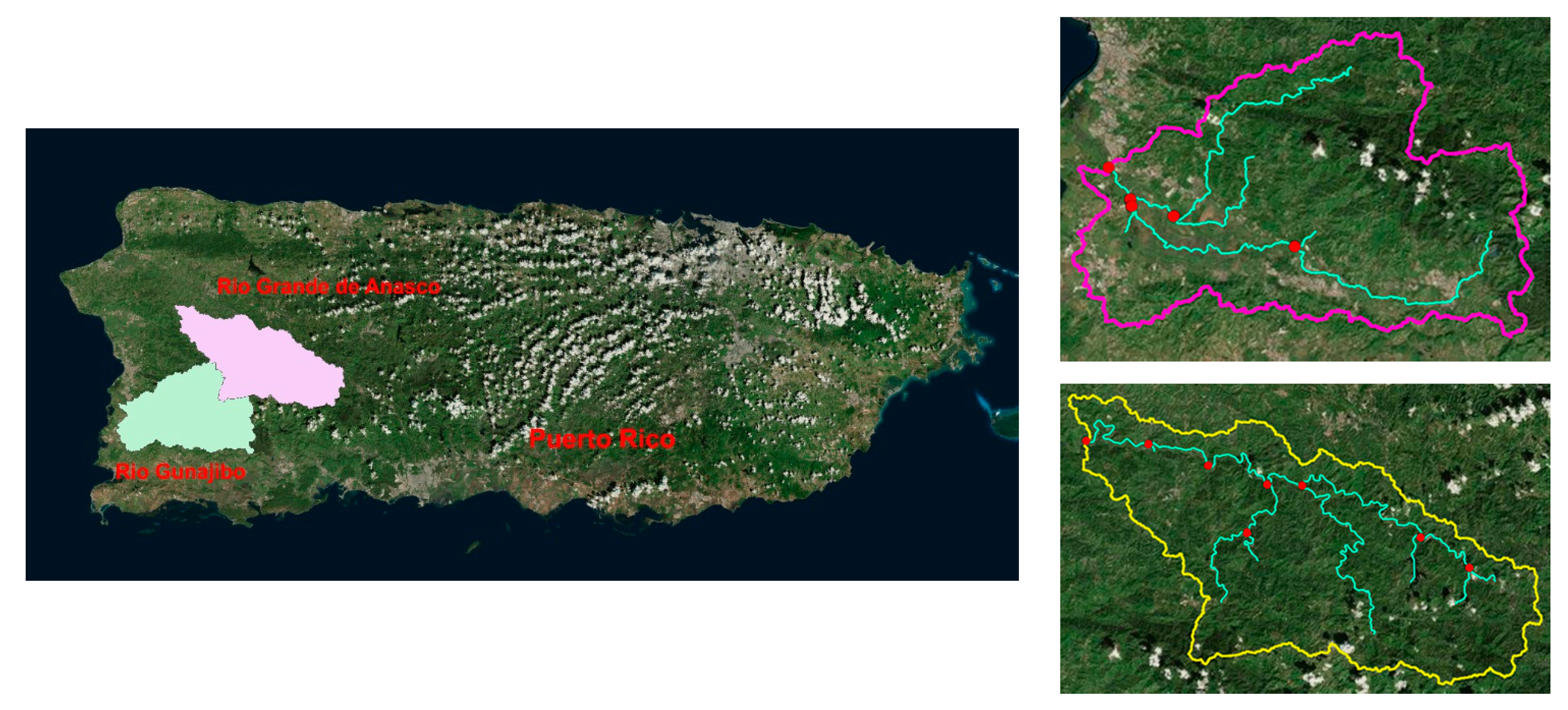
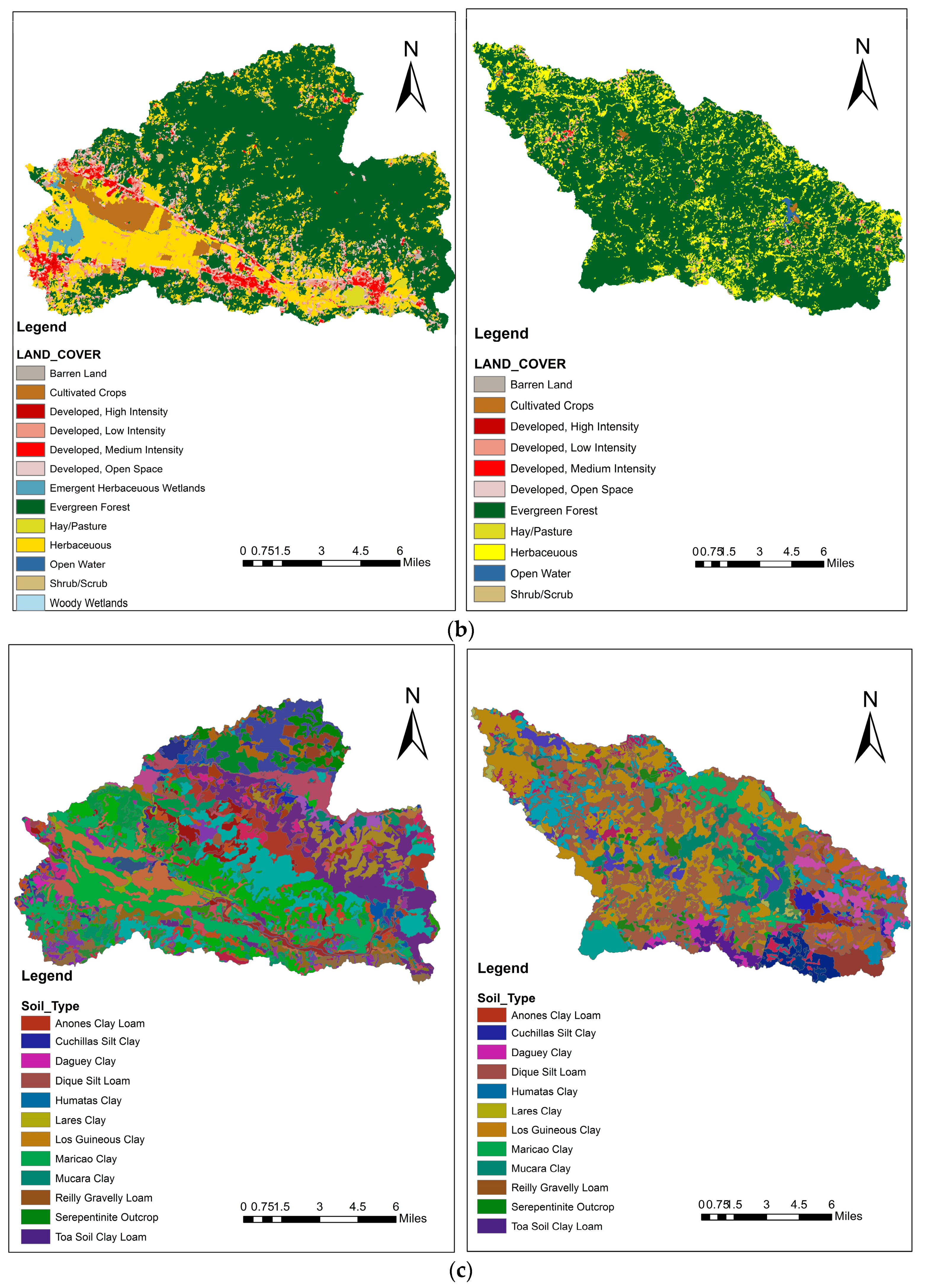
The study areas, Rio Guanajibo and Rio Grande de Añasco, are located in the western portion of the main island of Puerto Rico, USA (Figure 1). The watersheds are positioned between coordinate; northeast corner 18°19′14.16″ N–66°40′11.28″ W to southwest corner 17°58′5.88′′ N–67°11′20.04″ W and covers an area of 310.53 km2 and 252.52 km2, respectively. In general, both the sites receive annual average precipitation of 1687 mm. The annual average maximum and minimum temperature is 32 °C and 20 °C whereas the elevation ranges from −2 m to 370 mm above mean sea level. Evergreen forest is the dominant land use followed by herbaceous and hay in both the watershed.
2.2. Data Sources
SWAT interface for both the study area is created using input from various sources such as Digital Elevation Model (DEM) of 30 m resolution obtained from United States Geological Survey (USGS) SRTM (http://srtm.csi.cgiar.org/) (Figure 2a); land use land cover from national land cover database (NLCD) (http://databasin.org/datasets/) (Figure 2b); Soil Survey Geographic Database (SSURGO) soil map from National Resource Conservation Services (NRCS) (http://websoilsurvey.nrcs.usda.gov/) (Figure 2c); daily rainfall and temperature station data for the period 2008 to 2013 are collected from National Climatic Data Center (NCDC) (http://www.ncdc.noaa.gov/); solar radiation, relative humidity, wind speed are simulated on the basis of weather generated database by the model. Watershed outlet location and daily observed streamflow are collected from USGS gauge station (https://waterwatch.usgs.gov/). Remotely sensed satellite soil moisture data are collected from the Japan Aerospace Exploration Agency (JAXA) available on (http://global.jaxa.jp/). The soil moisture retrieved from AMSR2 on board GCOM-W1 that was launched in May 2012. The AMSR2 soil moisture data is available on the daily or monthly basis with a spatial resolution of 0.1° and 0.25° (10/25 km).
2.3. Model Application
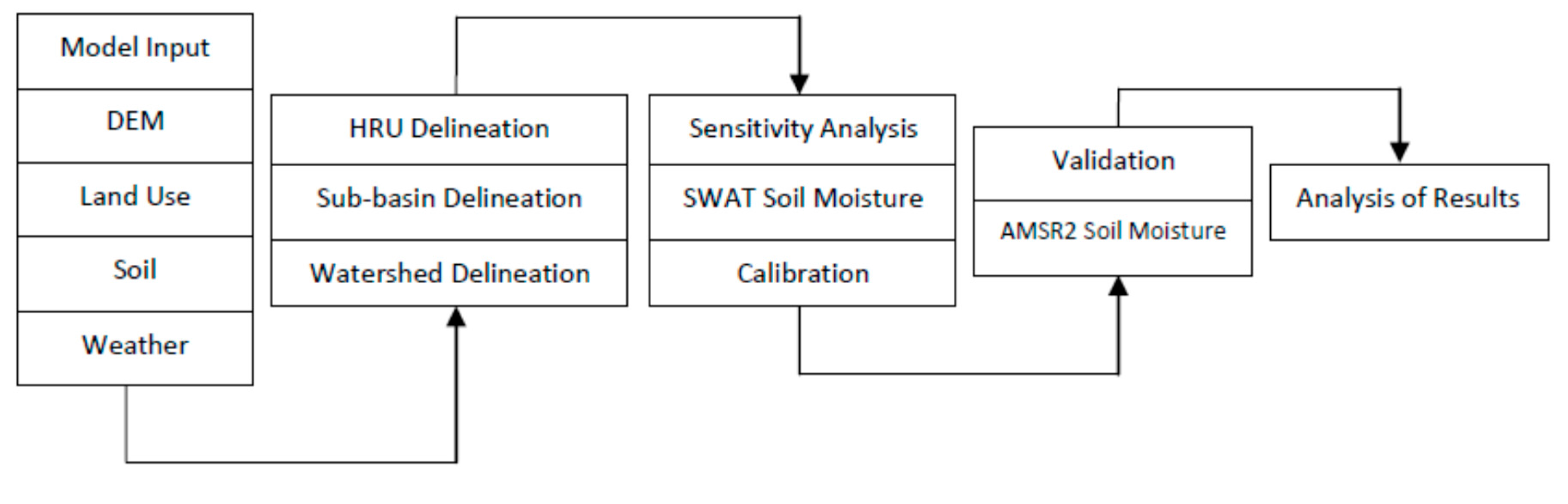
SWAT is a physically based semi-distributed basin scale model that uses parameter such as DEM, soil, land use, and climatic data for hydrological and climatological modeling on the daily or monthly basis [19,20,21]. Major model components include weather, hydrology, soil properties, plant growth, nutrients, and land management practices. The first stage of modeling involves watershed delineation. The delineated watershed is further subdivided into hydrologic response units (HRU) which is the unique combination of land use, soil, and slope. Each HRU in the model behaves differently for precipitation and temperature input [22]. For the given study each watershed is considered as the single basin to avoid complexity and to match the spatial resolution of AMSR2 soil moisture. The conversion of sub-basin to the single basin is made by changing the threshold limit in the model while the number of HRUs generated by the model remain same. The SWAT flow chart process is depicted in Figure 3.
2.4. Streamflow Generation
The hydrological cycle simulated by SWAT based on water balance equation and calculates water balance for each HRU.
where t is the time in days, SWt is the final soil water content, SW0 is the initial soil water content, Rday is amount of precipitation, Qsurf is the amount of surface runoff, ETa is the amount of evapotranspiration, Wseep is the amount of percolation, and Qgw is the amount of return flow. Thereafter, the aggregated results of various physical processes on HRU scale and can be integrated into basin level. Soil Conservation Services Curve Number method (SCS-CN) is used to calculate streamflow, infiltration, and canopy storage [23,24]. The lateral flow is simulated using a kinematic storage routing technique whereas return flow is simulated by considering shallow aquifer. In SWAT, Muskingum method is used for channel routing and potential evapotranspiration (PET) is estimated using the Penman–Monteith method [25]. The SWAT output includes water balance for each watersheds and flow at the outlet point.
2.5. Bias Correction
In Puerto Rico, a different network called Soil Climate Analysis Network (SCAN) run by NRCS is used to collect in situ data. Whereas measurement of soil moisture and temperature along with liquid precipitation, solar radiation, relative humidity, etc. at different depths, are assessed through the Snow Survey and Water Supply Forecasting Program (SSWSF). The data are compared to the data derived from GCOM-W1’s AMSR2 satellite. The units of the satellite data are originally v/v % before being converted to millimeters in order to obtain the same values in a unit of depth [26]. In order to retrieve the satellite data for the same coordinates as the in situ data, the minimum distance between two points, is calculated using the latitude and longitude of the ground station and the geographical coordinates included in the original satellite data [27]. This is done through the use of the Euclidean distance method (EDM). Once the data is retrieved, it is compared against the ground station data through a variety of statistical methods; although one discovery is that there is a very noticeable discrepancy between the in situ data and the satellite data. In order to account for this, any bias between the two sets of data is removed using a simple cumulative density function (CDF) that utilized the mean and standard deviation of both the ground station data and the satellite data. The following CDF is used in order to make the calculations
where θ is the final corrected soil moisture, 𝜇𝑔𝑟𝑜𝑢𝑛𝑑 is in situ soil moisture, 𝜎𝑠𝑎𝑡 is standard deviation of satellite soil moisture, 𝜎𝑔𝑟𝑜𝑢𝑛𝑑 is standard deviation of in situ soil moisture, 𝑠𝑎𝑡 is satellite soil moisture, 𝜇𝑠𝑎𝑡 is satellite soil moisture.
Once this is finished, the corrected data is then plotted again the original in situ data and shows that the satellite data is much closer matched than the original data.
2.6. Model Run
The model is run from the year 2008 to 2013 for both the watershed. The years 2008 and 2009 are used as a warm up period as this step is necessary to initialize the model and results of these are not considered in the model prediction. Another model is run for calibration and validation considering the parameter sensitivity from 2010 to 2013. Finally, the model performance is evaluated using statistical parameter such as the coefficient of determination (R2) which indicates a relationship between observed and model simulated values.
where n is a number of simulation, Qi is observed stream flow at time i, Si is simulated stream flow at time i, is mean observed streamflow, and is mean simulated streamflow [28].
3. Results and Discussion
3.1. Model Sensitivity Analysis
Sensitivity analysis is the process of determining the rate of change in model output with respect to changes in model input. Before the calibration sensitivity analysis is performed to reduce parameter uncertainty. The SWAT-CUP (calibration and uncertainty) incorporated with sequential uncertainty fitting (SUFI-2) is used for sensitivity analysis, calibration and validation of the model run [29,30]. The global sensitivity is performed for the given set of parameters which regresses the Latin hypercube generated parameter against the objective function value. The next step is the calibration process which is an effort to better parameterize a model to a given set of local conditions, thereby reducing prediction uncertainty [31,32,33,34]. Thirteen parameters are included in the calibration shown in Table 1.
Fitted value for each parameter is obtained by iterating previous parameter range. The relative sensitivity analysis is performed for both the study area of the Rio Guanajibo and the Rio Grande de Añasco respectively. The p value is used to measure the significance of sensitivity. The larger p value indicates lesser sensitive parameter whereas a value close or equal to zero indicates more sensitivity [35]. Parameters ALPHA_BNK, CN2, ALPHA_BF, GW_DELAY, and GW_REVAP are most sensitive parameters in the Rio Guanajibo basin, whereas ALPHA_BNK, GW_DELY, CN2, and GW_REVAP are most sensitive parameters in Rio Grande de Añasco basin. The most sensitive parameter has the effect on the calibration of streamflow and further change in the rest of the parameter value had no major effect on streamflow. The name and the values are listed in Table 2.
3.2. Calibration and Validation
The calibration is performed with 1000 simulations using data from January 2008 to December 2012 in which period 2008 to 2009 is used as warm-up period and not considered in the evaluation of the model prediction. In the preliminary assessment, the model streamflow results compared fairly well on a monthly basis with the observed value of streamflow. The range of a parameter is adjusted depending on the sensitivity analysis to match observed and simulated streamflow. The calibration yielded coefficients of determination R2 = 0.69 and R2 = 0.73 for the Rio Guanajibo and Rio Grande de Añasco watersheds respectively, shown in Figure 4. The temporal comparison between SWAT and AMSR2 satellite soil moisture is shown in Figure 5. In the Rio Guanajibo watershed, the value of AMSR2 soil moisture is higher in some months than SWAT soil moisture whereas, in the Rio Grande de Añasco watershed, the AMSR2 value is lower than SWAT soil moisture indicates a significant amount of bias in AMSR2 and SWAT soil moisture. This difference in soil moisture is due to change made in SWAT soil moisture depth to match the AMSR2 soil moisture depth.
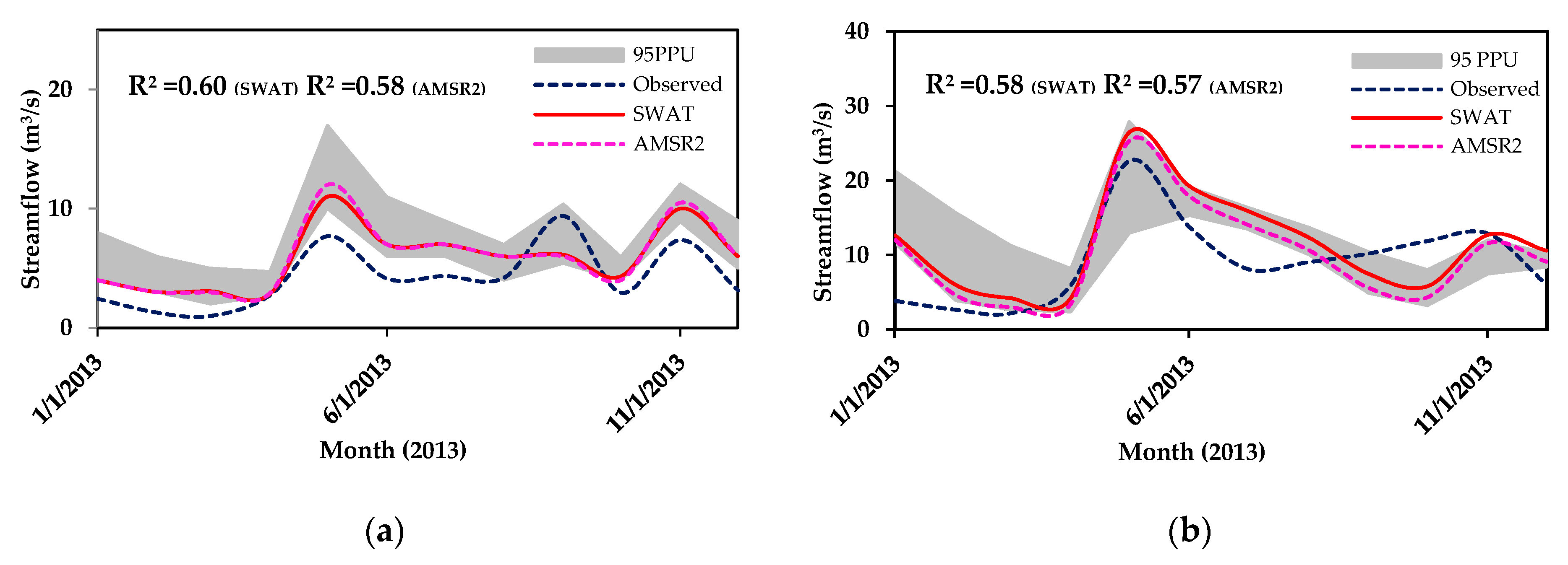
The same range of calibration parameters is used in order to perform validation for two different cases using data from year 2013. In the first case, model-generated soil moisture values are directly used for the validation. The R2 value estimated by the model is 0.60 for Rio Guanajibo and 0.58 for the Rio Grande de Añasco watershed shown in Figure 6. In the second case, AMSR2 values replace the model-generated values before being entered into the SWAT (HRU) layer. This leads to the generation of another model run that is then input into SUFI-2 for validation. The R2 values obtained for AMSR2 data are 0.58 and 0.57 in both the watersheds and are shown in Figure 6.
The comparison of validation results reveals a low influence of both SWAT and AMSR2 soil moisture values on the estimation of streamflow. Although the bias is seen in the soil moisture, streamflow is still less of an influence due to the parameter sensitivity. Soil moisture is less sensitive than the rest of the parameters in both the watershed hence indicate the lesser influence in streamflow. In some places, as a result, an observed streamflow does not match with SWAT streamflow due to the uncertainty involved either in model prediction or in climatic data such as precipitation and temperature, resulting in reduced R2 value. However, the estimated R2 value signifies an acceptable correlation between observed and estimated streamflow under varying land use, topography, and climatic conditions.
3.3. Streamflow Assessment
In the case of both watersheds, the streamflow assessment is based on the entire simulation period. In Rio Guanajibo, the model estimates mean annual rainfall of 2660.2 mm, PET of 1201.4 mm, evapotranspiration (ET) of 894.3 mm, water yield of 1702.57 mm, and baseflow/total flow of 71%. The model estimated values in Rio Grande de Añasco, mean annual rainfall of 2660.2 mm, PET of 1226.7 mm, ET of 1022.6 mm, water yield of 1496.47 mm, and baseflow/total flow of 78%. Añasco Both the watersheds are distributed with the same soil type and land use classification, which resulted in higher water yield value. The Higher ET value is obtained due to forest dominant land use in the watersheds. The forest land use covered in Rio Guanajibo is lower compared to Rio Grande de Añasco which indicates lower ET value in Rio Guanajibo watershed.
4. Conclusions
The study presents applicability of SWAT for calibration and validation of AMSR2 soil moisture in parts of Puerto Rico. The methodology evaluates assimilation of AMSR2 soil moisture in SWAT. However, there is still a scope for improvement in results between observed and simulated streamflow in the Rio Guanajibo and the Rio Grande de Añasco watersheds. The sensitivity analysis accounting for streamflow calibration has shown variations between the parameter range, which had been initialized for model calibration. Thus, it indicated that parameters ALPHA_BNK, CN2, ALPHA_BF, GW_REVAP, and GW_DELAY are sensitive and have a great impact on the stream flow. The SUFI-2 procedure tries to minimize the difference between observed and measured streamflow data. Further results can be enhanced using model run on daily weather data and satellite soil moisture data over a longer period of time. The overall effect of AMSR2 soil moisture in SWAT is negligible, thus suggesting that the use of AMSR2 soil moisture will be effective when soil moisture is the most sensitive parameter in the SWAT. The soil moisture replacement technique improved model efficiency and considered a larger temporal variation. Finally, results revealed that the SWAT fusion with AMSR2 soil moisture is capable of simulating streamflow and could be effectively applied in hydrological modeling.
Acknowledgments
Authors are thankful to Reza Khanbilvardi, Center Director, NOAA-CREST, The City College of the City University of New York for providing workstation to carry out the study. Authors are also thankful to the authorities of the SGGS Institute of Engineering and Techonology, Center of Excellence Signal and Image processing and Technical Education Quality Improvement Programme (Government of India) for financial support. This study was partially supported by NOAA grant NA14NES4320003 (Cooperative Institute for Climate and Satellites -CICS) at the University of Maryland/ESSIC. The statements contained within the manuscript/research article are not the opinions of the funding agency or the United States government but reflect the author’s opinions.
Author Contributions
Aditya P. Nilawar, Cassandra P. Calderella, Tarendra Y. Lakhankar, Milind L. Waikar, and Jonathan Munoz contributed to data collection and data analysis. All authors have read and corrected the paper.
Conflicts of Interest
The authors declare no conflict of interest.
References
- Walker, J.P.; Dumedah, G.; Monerris, A.; Gao, Y.; Rüdiger, C.; Wu, X.; Panciera, R.; Merlin, O.; Pipunic, R.; Ryu, D.; et al. High resolution soil moisture mapping. In Computing Ethics: A Multicultural Approach; Chapman & Hall/CRC: London, UK, 2016; p. 45. [Google Scholar]
- Dorigo, W.A.; Wagner, W.; Hohensinn, R.; Hahn, S.; Paulik, C.; Xaver, A.; Gruber, A.; Drusch, M.; Mecklenburg, S.; van Oevelen, P.; et al. The International Soil Moisture Network: A data hosting facility for global in situ soil moisture measurements. Hydrol. Earth Syst. Sci. 2011, 15, 1675–1698. [Google Scholar] [CrossRef]
- Laiolo, P.; Gabellani, S.; Pulvirenti, L.; Boni, G.; Rudari, R.; Delogu, F.; Silvestro, F.; Campo, L.; Fascetti, F.; Pierdicca, N.; et al. Validation of remote sensing soil moisture products with a distributed continuous hydrological model. In Proceedings of the 2014 IEEE International Geoscience and Remote Sensing Symposium (IGARSS), Quebec City, QC, Canada, 13–18 July 2014; pp. 3319–3322. [Google Scholar]
- Merlin, O.; Walker, J.; Panciera, R.; Young, R.; Kalma, J.; Kim, E. Soil moisture measurement in heterogeneous terrain. In Proceedings of the Congress Theme of Land, Water and Environmental Management: Integrated Systems for Sustainability, Christchurch, New Zealand, 10–13 December 2007; pp. 2604–2610. [Google Scholar]
- Wanders, N.; Karssenberg, D.; De Roo, A.; De Jong, S.M.; Bierkens, M.F.P. The suitability of remotely sensed soil moisture for improving operational flood forecasting. Hydrol. Earth Syst. Sci. 2014, 18, 2343–2357. [Google Scholar] [CrossRef]
- Kumar, S.V.; Peters-Lidard, C.D.; Santanello, J.A.; Reichle, R.H.; Draper, C.S.; Koster, R.D.; Nearing, G.; Jasinski, M.F. Evaluating the utility of satellite soil moisture retrievals over irrigated areas and the ability of land data assimilation methods to correct for unmodeled processes. Hydrol. Earth Syst. Sci. 2015, 19, 4463–4478. [Google Scholar]
- Liu, L. Soil Moisture Mapping in Vegetated Area Using Landsat and Envisat ASAR Data. In Proceedings of the 1st International Electronic Conference on Remote Sensing, Dresden, Germany, 22 June–5 July 2015; pp. 1–7. [Google Scholar]
- Martínez-Fernández, J.; González-Zamora, A.; Sánchez, N.; Gumuzzio, A.; Herrero-Jiménez, C.M. Satellite soil moisture for agricultural drought monitoring: Assessment of the SMOS derived Soil Water Deficit Index. Remote Sens. Environ. 2016, 177, 277–286. [Google Scholar] [CrossRef]
- Entekhabi, D.; Njoku, E.G.; O’Neill, P.E.; Kellogg, K.H.; Crow, W.T.; Edelstein, W.N.; Entin, J.K.; Goodman, S.D.; Jackson, T.J.; Johnson, J.; et al. The soil moisture active passive (SMAP) mission. Proc. IEEE 2010, 98, 704–716. [Google Scholar] [CrossRef]
- Kolassa, J.; Gentine, P.; Prigent, C.; Aires, F.; Alemohammad, S.H. Soil moisture retrieval from AMSR-E and ASCAT microwave observation synergy. Part 2: Product evaluation. Remote Sens. Environ. 2017, 195, 202–217. [Google Scholar] [CrossRef]
- Ban, Y.; Marullo, S.; Eklundh, L. European Remote Sensing: Progress, challenges, and opportunities. Int. J. Remote Sens. 2017, 38, 1759–1764. [Google Scholar] [CrossRef]
- Zhuo, L.; Han, D. Hydrological Evaluation of Satellite Soil Moisture Data in Two Basins of Different Climate and Vegetation Density Conditions. Adv. Meteorol. 2017, 2017, 1086456. [Google Scholar] [CrossRef]
- Gruhier, C.; de Rosnay, P.; Hasenauer, S.; Holmes, T.; de Jeu, R.; Kerr, Y.; Mougin, E.; Njoku, E.; Timouk, F.; Wagner, W.; et al. Soil moisture active and passive microwave products: Intercomparison and evaluation over a Sahelian site. Hydrol. Earth Syst. Sci. 2010, 14, 141–156. [Google Scholar] [CrossRef] [Green Version]
- Xiao, Z.; Jiang, L.; Zhu, Z.; Wang, J.; Du, J. Spatially and temporally complete satellite soil moisture data based on a data assimilation method. Remote Sens. 2016, 8, 49. [Google Scholar] [CrossRef]
- Wu, Q.; Liu, H.; Wang, L.; Deng, C. Evaluation of AMSR2 soil moisture products over the contiguous United States using in situ data from the International Soil Moisture Network. Int. J. Appl. Earth Obs. Geoinf. 2016, 45, 187–199. [Google Scholar] [CrossRef]
- Zhang, X.; Zhang, T.; Zhou, P.; Shao, Y.; Gao, S. Validation Analysis of SMAP and AMSR2 Soil Moisture Products over the United States Using Ground-Based Measurements. Remote Sens. 2017, 9, 104. [Google Scholar] [CrossRef]
- Brocca, L.; Ciabatta, L.; Massari, C.; Camici, S.; Tarpanelli, A. Soil Moisture for Hydrological Applications: Open Questions and New Opportunities. Water 2017, 9, 140. [Google Scholar] [CrossRef]
- Zhuo, L.; Han, D. The Relevance of Soil Moisture by Remote Sensing and Hydrological Modelling. Procedia Eng. 2016, 154, 1368–1375. [Google Scholar] [CrossRef]
- Arnold, J.G.; Shrinivasan, R.; Muttiah, R.S.; Williams, J.R. Large area hdyrologic modeling and assessment part I: Model devlopment. J. Am. Water Resour. Assoc. 1998, 34, 73–89. [Google Scholar] [CrossRef]
- Olivera, F.; Valenzuela, M.; Srinivasan, R.; Choi, J.; Cho, H.; Koka, S.; Agrawal, A. ARCGIS-SWAT: A geodata model and GIS interface for SWAT1. JAWRA J. Am. Water Resour. Assoc. 2006, 42, 295–309. [Google Scholar] [CrossRef]
- Setegn, S.G.; Srinivasan, R.; Dargahi, B. Hydrological modelling in the Lake Tana Basin, Ethiopia using SWAT model. Open Hydrol. J. 2008, 2, 49–62. [Google Scholar] [CrossRef]
- Yacoub, C.; Foguet, A.P. Slope effects on SWAT modeling in a mountainous basin. J. Hydrol. Eng. 2012, 18, 1663–1673. [Google Scholar] [CrossRef]
- Gupta, P.K.; Punalekar, S.; Panigrahy, S.; Sonakia, A.; Parihar, J.S. Runoff modeling in an agro-forested watershed using remote sensing and GIS. J. Hydrol. Eng. 2011, 17, 1255–1267. [Google Scholar] [CrossRef]
- Williams, J.R.; Kannan, N.; Wang, X.; Santhi, C.; Arnold, J.G. Evolution of the SCS runoff curve number method and its application to continuous runoff simulation. J. Hydrol. Eng. 2011, 17, 1221–1229. [Google Scholar] [CrossRef]
- Santhi, C.; Srinivasan, R.; Arnold, J.G.; Williams, J.R. A modeling approach to evaluate the impacts of water quality management plans implemented in a watershed in Texas. Environ. Model. Softw. 2006, 21, 1141–1157. [Google Scholar] [CrossRef]
- Rajib, M.A.; Merwade, V.; Yu, Z. Multi-objective calibration of a hydrologic model using spatially distributed remotely sensed/in situ soil moisture. J. Hydrol. 2016, 536, 192–207. [Google Scholar] [CrossRef]
- Van Arkel, Z.; Kaleita, A.L. Identifying sampling locations for field-scale soil moisture estimation using K-means clustering. Water Resour. Res. 2014, 50, 7050–7057. [Google Scholar] [CrossRef]
- Srinivasan, R.; Zhang, X.; Arnold, J. SWAT ungaged: Hydrological budget and crop yield predictions in the Upper Mississipp River basin. Trans. Am. Soc. Agric. Biol. Eng. 2010, 53, 1533–1546. [Google Scholar] [CrossRef]
- Abbaspour, K.C.; Vejdani, M.; Haghighat, S.; Yang, J. SWAT-CUP calibration and uncertainty programs for SWAT. In Proceedings of the MODSIM 2007 International Congress on Modelling and Simulation, Christchurch, New Zealand, December 2007; Modelling and Simulation Society of Australia and New Zealand Inc. (MSSANZ): Christchurch, New Zealand, 2007; pp. 1596–1602. [Google Scholar]
- Arnold, J.G.; Moriasi, D.N.; Gassman, P.W.; Abbaspour, K.C.; White, M.J.; Srinivasan, R.; Santhi, C.; Harmel, R.D.; Van Griensven, A.; Van Liew, M.W.; et al. SWAT: Model use, calibration, and validation. Trans. ASABE 2012, 55, 1491–1508. [Google Scholar] [CrossRef]
- Baker, T.J.; Miller, S.N. Using the Soil and Water Assessment Tool (SWAT) to assess land use impact on water resources in an East African watershed. J. Hydrol. 2013, 486, 100–111. [Google Scholar] [CrossRef]
- Xue, C.; Chen, B.; Wu, H. Parameter uncertainty analysis of surface flow and sediment yield in the Huolin Basin, China. J. Hydrol. Eng. 2013, 19, 1224–1236. [Google Scholar] [CrossRef]
- Jha, M.K. Evaluating hydrologic response of an agricultural watershed for watershed analysis. Water 2011, 3, 604–617. [Google Scholar] [CrossRef]
- Rafiei Emam, A.; Kappas, M.; Linh, N.H.K.; Renchin, T. Hydrological Modeling and Runoff Mitigation in an Ungauged Basin of Central Vietnam Using SWAT Model. Hydrology 2017, 4, 16. [Google Scholar] [CrossRef]
- Schuol, J.; Abbaspour, K.C. Calibration and uncertainty issues of a hydrological model (SWAT) applied to West Africa. Adv. Geosci. 2006, 9, 137–143. [Google Scholar] [CrossRef]
Figure 1.
Location of the Rio Guanajibo and Rio Grande de Añasco sub-basins in Puerto Rico, USA. The study area showing stream networks, outlet points, and basin boundary.
Figure 1.
Location of the Rio Guanajibo and Rio Grande de Añasco sub-basins in Puerto Rico, USA. The study area showing stream networks, outlet points, and basin boundary.

Figure 2.
Input data for SWAT (a) DEM elevation of the area ranges from 3 m to 1183 m; (b) LULC classifications in the area; (c) Soil type.
Figure 2.
Input data for SWAT (a) DEM elevation of the area ranges from 3 m to 1183 m; (b) LULC classifications in the area; (c) Soil type.
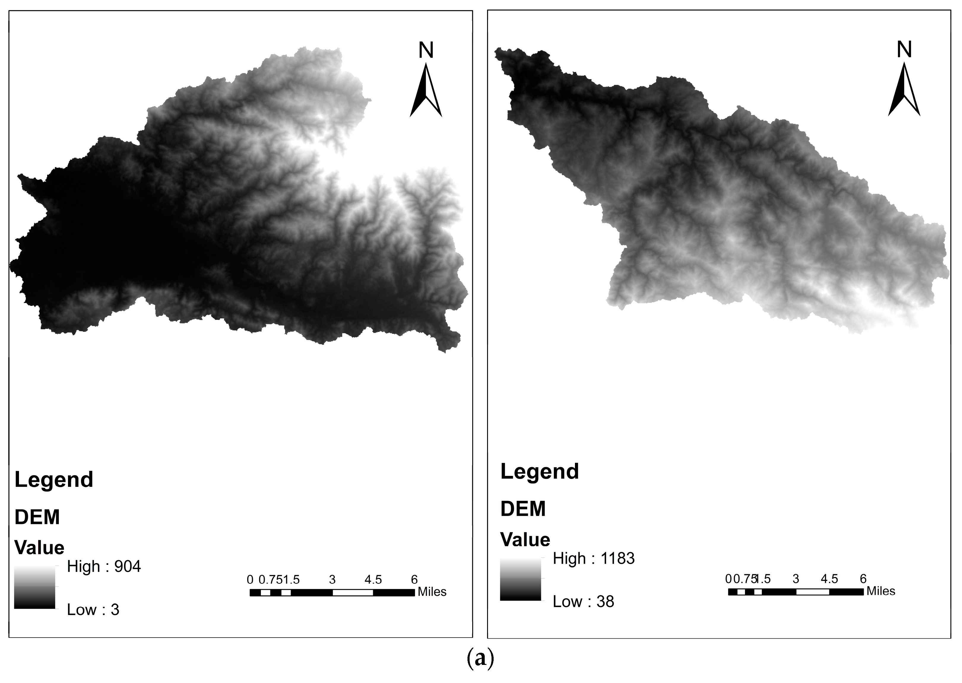

Figure 3.
Flow chart of methodology for streamflow measurement using SWAT in Puerto Rico, USA.

Figure 4.
Calibration of observed and simulated streamflow (m3/s) during period (January 2010–December 2012): (a) Rio Guanajibo watershed, and (b) Rio Grande de Añasco watershed, Puerto Rico, USA.
Figure 4.
Calibration of observed and simulated streamflow (m3/s) during period (January 2010–December 2012): (a) Rio Guanajibo watershed, and (b) Rio Grande de Añasco watershed, Puerto Rico, USA.
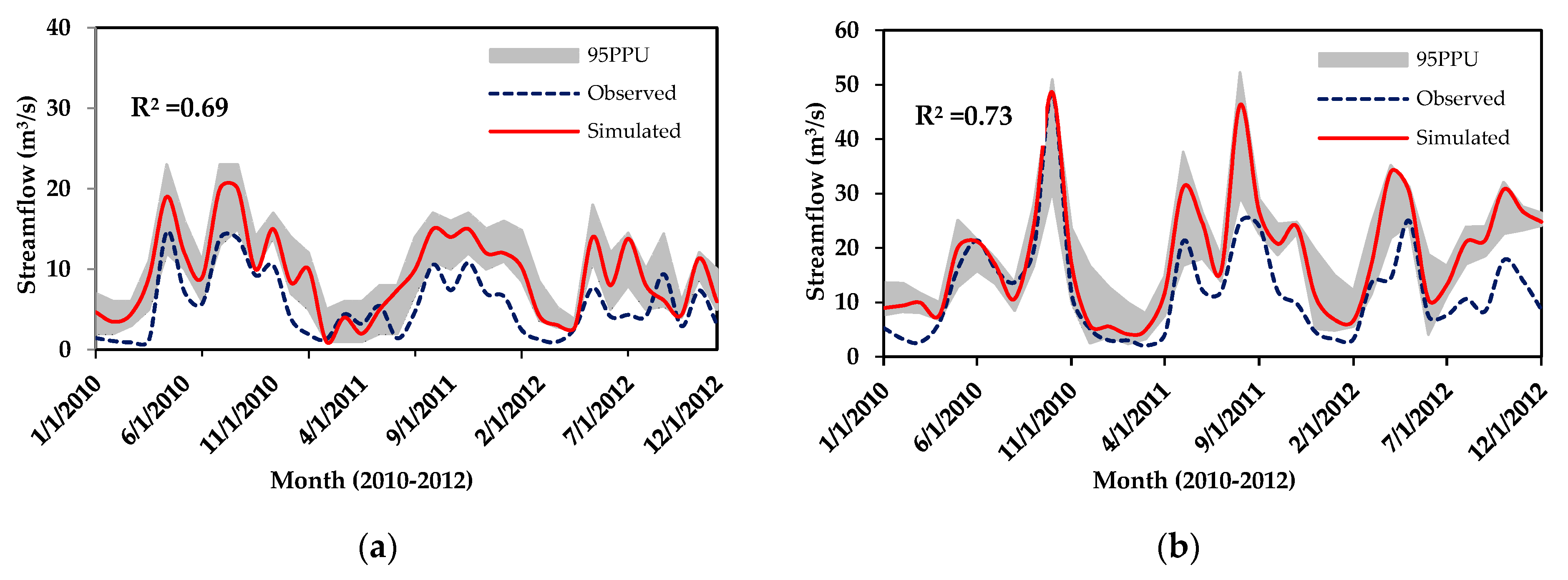
Figure 5.
Comparison of SWAT and AMSR2 soil moisture (mm) during period (January 2013–December 2013): (a) Rio Guanajibo watershed, and (b) Rio Grande de Añasco watershed, Puerto Rico, USA.
Figure 5.
Comparison of SWAT and AMSR2 soil moisture (mm) during period (January 2013–December 2013): (a) Rio Guanajibo watershed, and (b) Rio Grande de Añasco watershed, Puerto Rico, USA.
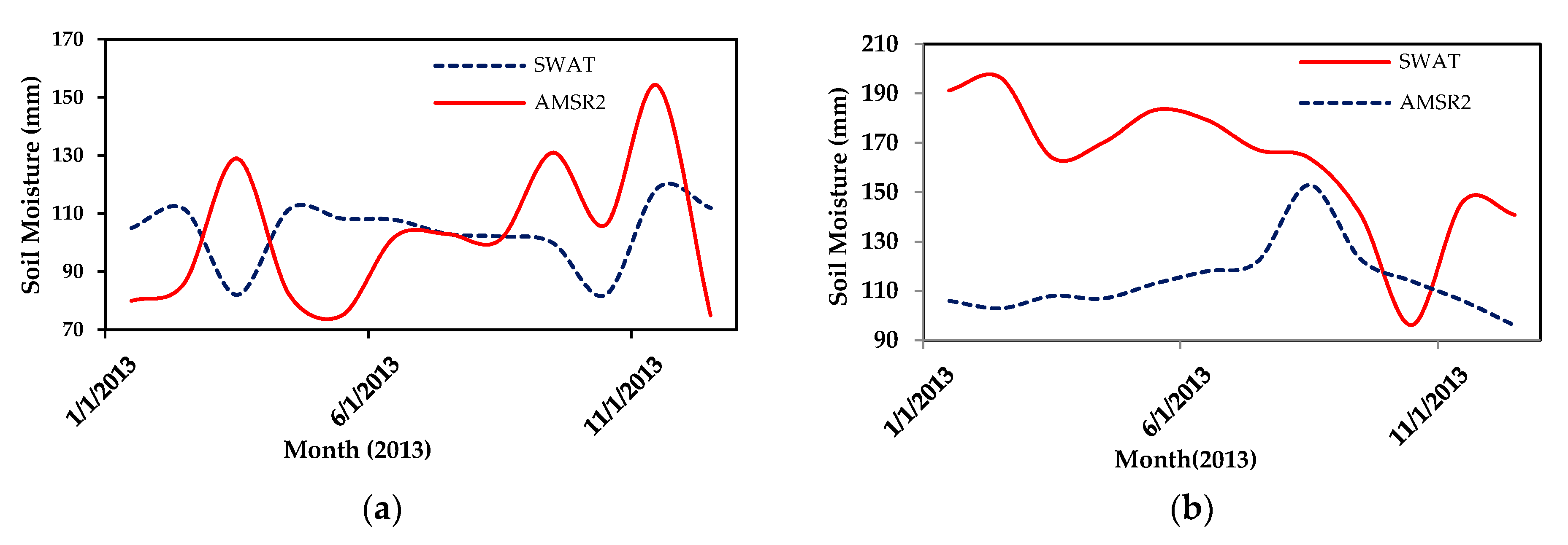
Figure 6.
Validation of SWAT and AMSR2 streamflow (m3/s) with observed streamflow (m3/s) during period (January 2013–December 2013): (a) Rio Guanajibo watershed and, (b) Rio Grande de Añasco watershed, Puerto Rico, USA.
Figure 6.
Validation of SWAT and AMSR2 streamflow (m3/s) with observed streamflow (m3/s) during period (January 2013–December 2013): (a) Rio Guanajibo watershed and, (b) Rio Grande de Añasco watershed, Puerto Rico, USA.


Table 1.
SWAT parameters including initial and fitted value for streamflow calibration
| Parameter * | Parameter Name | Initial Range | Final Range for Guanajibo | Fitted Values for Guanajibo | Final Range for Añasco | Fitted Values for Añasco |
|---|---|---|---|---|---|---|
| r_CN2 | SCS runoff curve number | −0.2 to 0.2 | −0.36 to −0.45 | −0.40 | −0.28 to −0.17 | −0.24 |
| v_ALPHA_BF | Base flow alpha factor (days) | 0 to 1 | 0 .57 to 1 | 0.72 | 0.69 to 1 | 0.7 |
| a_GW_DELAY | Groundwater delay time (days) | 30 to 450 | 31 to 256 | 198 | 20 to 58 | 38 |
| a_GWQMN | Threshold depth of water in shallow aquifer for return flow to occur (mm) | 0 to 2 | 1.3 to 2 | 1.7 | 1.43 to 2 | 1.9 |
| v_GW_REVAP | Groundwater revap. coefficient | 0 to 0.3 | 0.19 to 0.3 | 0.24 | 0.16 to 0.25 | 0.2 |
| v_ESCO | Soil evaporation compensation factor | 0.5 to 1 | 0.75 to 1 | 0.74 | 0.74 to 0.86 | 0.76 |
| v_CH_N2 | Manning’s n value for main channel | 0 to 0.3 | 0.10 to 0.27 | 0.2 | 0.20 to 0.29 | 0.25 |
| v_CH_K2 | Effective hydraulic conductivity in the main channel (mm/h) | 5 to 130 | 52 to 85 | 61 | 79 to 130 | 94 |
| v_ALPHA_BNK | Base flow alpha factor for bank storage (days) | 0 to 1 | 0.01 to 0.22 | 0.1 | 0.01 to 0.17 | 0.06 |
| r_SOL_AWC | Soil available water storage capacity (mm H2O/mm soil) | −0.2 to 0.4 | 0.05 to 0.36 | 0.35 | 0.13 to 0.32 | 0.24 |
| r_SOL_K | Soil conductivity (mm/h) | −0.8 to 0.8 | 0.14 to 0.71 | 0.6 | 0.37 to 0.79 | 0.6 |
| r_SOL_BD | Moist bulk density of first soil layer (Mg/m3) | −0.5 to 0.6 | 0.26 to 0.6 | 0.41 | 0.1 to 0.49 | 0.16 |
| v_SFTMP | Snow fall temperature(°C) | −5 to 5 | −4.34 to 1.73 | −1.3 | 1.44 to 4.67 | 1.8 |
* The changes in the parameter values are applied by (r) relative change means existing parameter value is to be multiplied with (1 + fitted value), (v) variable means the existing parameter value to be replaced by fitted value, (a) absolute means existing parameter value is added to a fitted value.
Table 2.
Global sensitivity analysis for 13 parameters in Rio Guanajibo and Rio Grande de Añasco watershed. Smaller P value indicates more parameter sensitivity.
Table 2.
Global sensitivity analysis for 13 parameters in Rio Guanajibo and Rio Grande de Añasco watershed. Smaller P value indicates more parameter sensitivity.
| Rio Guanajibo | Rio Grande de Añasco | ||||
|---|---|---|---|---|---|
| Parameter | Rank | p Value | Parameter | Rank | p Value |
| ALPHA_BNK | 1 | 0.00 | ALPHA_BNK | 1 | 0.00 |
| CN2 | 2 | 0.00 | GW_DELAY | 2 | 0.00 |
| ALPHA_BF | 3 | 0.02 | CN2 | 3 | 0.03 |
| GW_DELAY | 4 | 0.02 | SFTMP | 4 | 0.03 |
| GW_REVAP | 5 | 0.05 | GW_REVAP | 5 | 0.04 |
| CH_K2 | 6 | 0.15 | SOL_AWC | 6 | 0.26 |
| SOL_BD | 7 | 0.27 | SOL_K | 7 | 0.40 |
| SOL_AWC | 8 | 0.34 | ALPHA_BF | 8 | 0.50 |
| SOL_K | 9 | 0.38 | GWQMN | 9 | 0.54 |
| ESCO | 10 | 0.47 | ESCO | 10 | 0.61 |
| GWQMN | 11 | 0.56 | CH_K2 | 11 | 0.70 |
| SFTMP | 12 | 0.64 | CH_N2 | 12 | 0.77 |
| CH_N2 | 13 | 0.75 | SOL_BD | 13 | 0.85 |
© 2017 by the authors. Licensee MDPI, Basel, Switzerland. This article is an open access article distributed under the terms and conditions of the Creative Commons Attribution (CC BY) license (http://creativecommons.org/licenses/by/4.0/).
Share and Cite
MDPI and ACS Style
Nilawar, A.P.; Calderella, C.P.; Lakhankar, T.Y.; Waikar, M.L.; Munoz, J. Satellite Soil Moisture Validation Using Hydrological SWAT Model: A Case Study of Puerto Rico, USA. Hydrology 2017, 4, 45. https://doi.org/10.3390/hydrology4040045
AMA Style
Nilawar AP, Calderella CP, Lakhankar TY, Waikar ML, Munoz J. Satellite Soil Moisture Validation Using Hydrological SWAT Model: A Case Study of Puerto Rico, USA. Hydrology. 2017; 4(4):45. https://doi.org/10.3390/hydrology4040045
Chicago/Turabian StyleNilawar, Aditya P., Cassandra P. Calderella, Tarendra Y. Lakhankar, Milind L. Waikar, and Jonathan Munoz. 2017. "Satellite Soil Moisture Validation Using Hydrological SWAT Model: A Case Study of Puerto Rico, USA" Hydrology 4, no. 4: 45. https://doi.org/10.3390/hydrology4040045
Note that from the first issue of 2016, this journal uses article numbers instead of page numbers. See further details here.