Nonlinear Effects on the Convergence of Picard and Newton Iteration Methods in the Numerical Solution of One-Dimensional Variably Saturated–Unsaturated Flow Problems

Abstract
:1. Introduction
2. Numerical Formulation
2.1. Finite Element Model
2.2. Linearization Techniques
2.2.1. Newton and Picard Schemes
2.3. Characteristic Equations
2.3.1. Van Genuchten Model
2.3.2. The Brooks-Corey Model
2.4. Implementation
3. Numerical Results
3.1. Problem 1
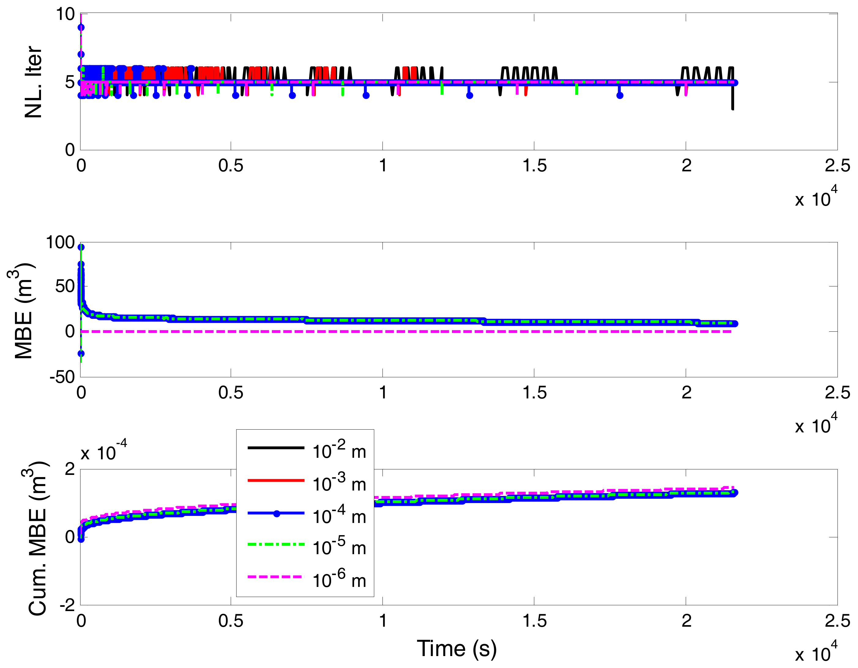
3.2. Problem 2
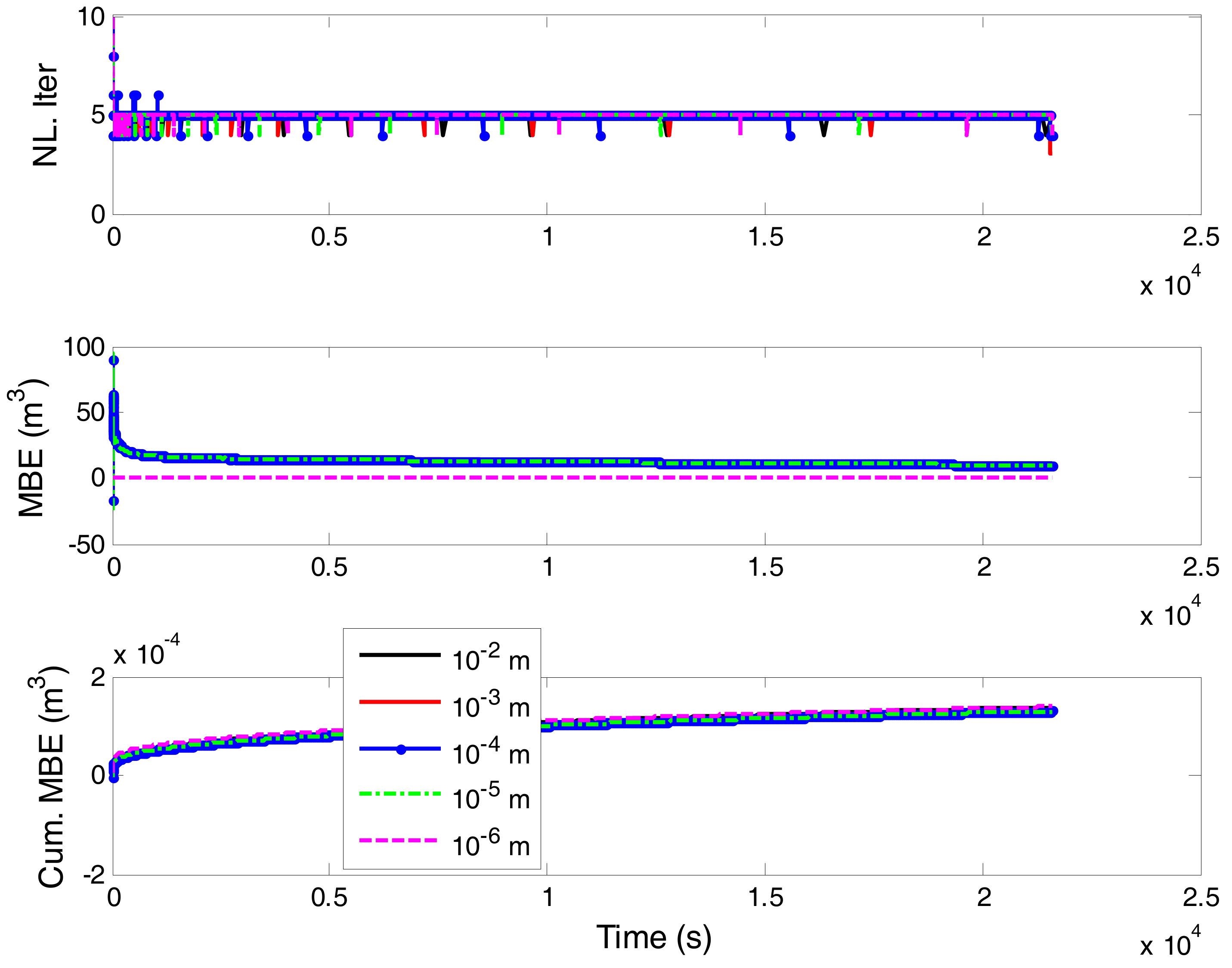
3.3. Problem 3
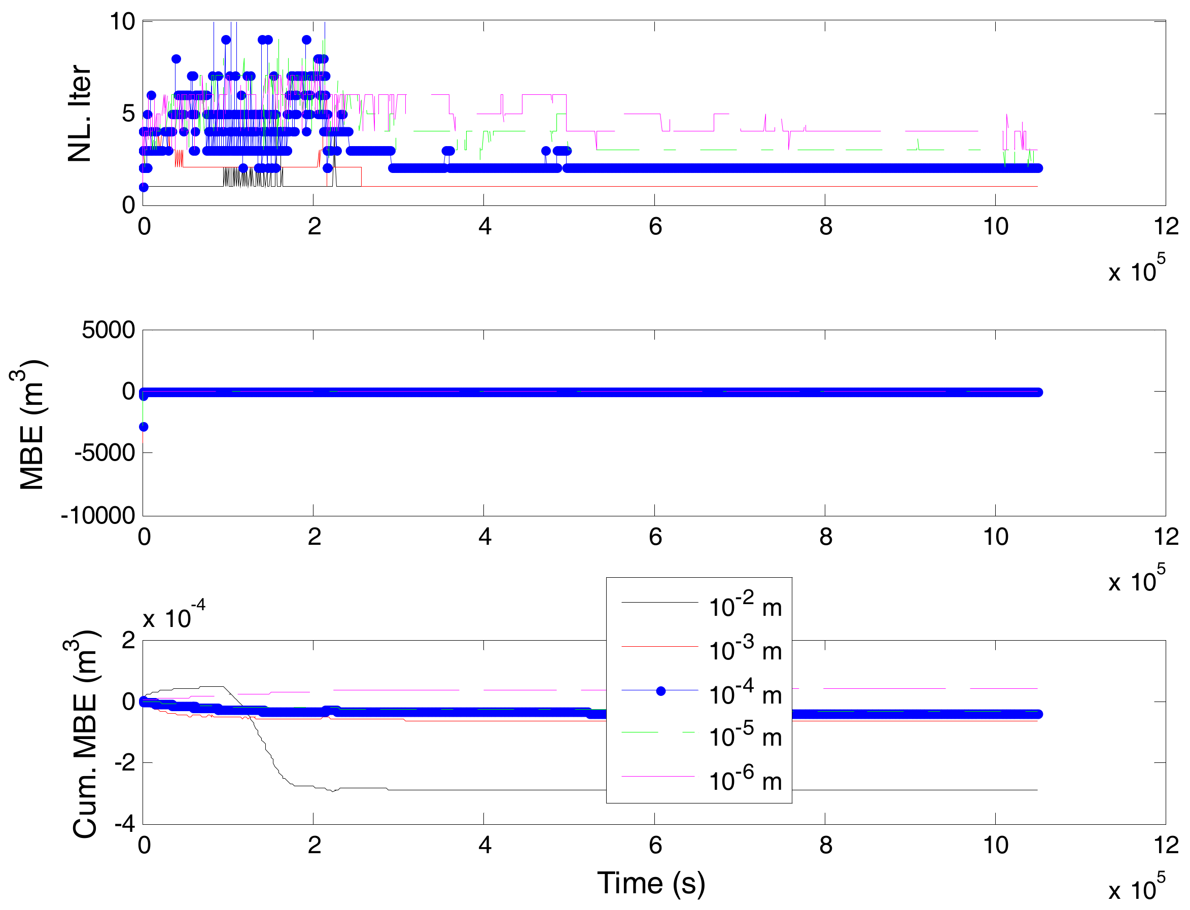
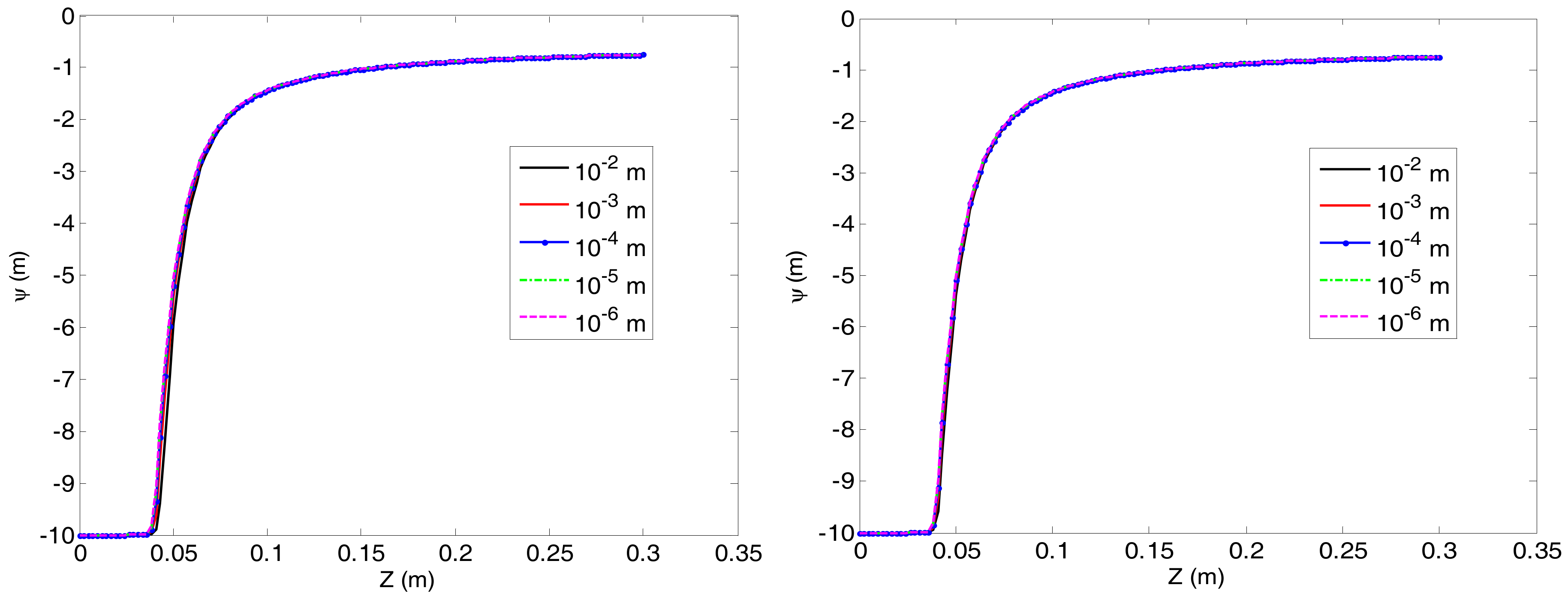
3.4. Problem 4
4. Conclusions
Acknowledgments
Author Contributions
Conflicts of Interest
References
- Richards’, L.A. Capillary conduction of liquids in porous media. Physics 1931, 1, 318–333. [Google Scholar] [CrossRef]
- Celia, M.A.; Bouloutas, E.T.; Zarba, R.L. A General mass-conservative numerical solution for the unsaturated flow equation. Water Resour. Res. 1990, 26, 1483–1496. [Google Scholar] [CrossRef]
- Clement, T.P.; Wise, W.R.; Molz, F.J. A physically base, two-dimensional, finite difference algorithm for modeling variably saturated flow. J. Hydrol. 1994, 161, 71–90. [Google Scholar] [CrossRef]
- Fassino, C.; Manzini, G. Fast-secant algorithms for the non-linear Richards’ Equation. Commun. Numer. Methods Eng. 1998, 14, 921–930. [Google Scholar] [CrossRef]
- Huang, K.; Mohanty, B.; van Genuchten, M. A new convergence criterion for the modified iteration method for solving the variably saturated flow equation. J. Hydrol. 1996, 178, 69–91. [Google Scholar] [CrossRef]
- D’Haese, C.M.F.; Putti, M.; Paniconi, C.; Verhoest, N.E.C. Assessment of adaptive and heuristic time stepping for variably saturated flow. Int. J. Numer. Methods Fluids 2007, 53, 1173–1193. [Google Scholar] [CrossRef]
- Casulli, V.; Zanolli, P. A nested Newton-type algorithm for finite volume methods solving Richards’ equation in mixed form. SIAM J. Sci. Comput. 2010, 32, 2255–2273. [Google Scholar] [CrossRef]
- Severino, G.; Scarfato, M.; Toraldo, G. Mining geostatistics to quantify the spatial variability of certain soil flow properties. Procedia Comput. Sci. 2016, 98, 419–424. [Google Scholar] [CrossRef]
- Severino, G.; Scarfato, M.; Comegna, A. Stochastic analysis of unsaturated steady flows above the water table. Water Resour. Res. 2017, 53, 6687–6708. [Google Scholar] [CrossRef]
- Miller, C.T.; Williams, G.A.; Kelly, C.T.; Tocci, M.D. Robust solution of Richards’ equation for nonuniform porous media. Water Resour. Res. 1998, 34, 2599–2610. [Google Scholar] [CrossRef]
- Bergamaschi, L.; Putti, M. Mixed finite elements and Newton-type linearizations for the solution of Richards’ equation. Int. J. Numer. Methods Eng. 1999, 45, 1025–1046. [Google Scholar] [CrossRef]
- Forsyth, P.A.; Wu, Y.S.; Pruess, K. Robust numerical methods for saturated-unsaturated flow with dry initial conditions in heterogeneous media. Adv. Water Resour. 1995, 18, 25–38. [Google Scholar] [CrossRef]
- Kavetski, D.; Binning, P.; Sloan, S.W. Adaptive time stepping and error control in a mass conservative numerical solution of the mixed form of Richards equation. Adv. Water Resour. 2001, 24, 595–605. [Google Scholar] [CrossRef]
- Manzini, G.; Ferraris, S. Mass-conservative finite volume methods in 2-D unstructured grids for the Richards’ equation. Adv. Water Resour. 2004, 27, 1199–1215. [Google Scholar] [CrossRef]
- McBride, D.; Cross, M.; Croft, N.; Bennett, C.; Gebhardt, J. Computational modeling of variably saturated flow in porous media with complex three-dimensional geometries. Int. J. Numer. Methods Fluids 2006, 50, 1085–1117. [Google Scholar] [CrossRef]
- Paniconi, C.; Aldama, A.A.; Wood, E.F. Numerical evaluation of iterative and noniterative methods for the solution of the nonlinear Richards’ equation. Water Resour. Res. 1991, 27, 1147–1163. [Google Scholar] [CrossRef]
- Paniconi, C.; Putti, M. A comparison of Picard and Newton iteration in the numerical solution of multidimensional variably saturated flow problems. Water Resour. Res. 1994, 30, 3357–3374. [Google Scholar] [CrossRef]
- Kelly, C.T.; Miller, C.T.; Tocci, M.D. Termination of Newton/Chord iteration and the method of lines. SIAM J. Sci. Comput. 1998, 19, 280–290. [Google Scholar] [CrossRef]
- Van Genuchten, M.T. A closed-form equation for predicting the hydraulic conductivity of unsaturated soils. Soil Sci. Soc. Am. J. 1980, 44, 892–898. [Google Scholar] [CrossRef]
- Brooks, R.H.; Corey, A.T. Properties of porous media affecting fluid flow. J. Irrig. Drain. Div. Am. Soc. Civ. Eng. 1966, 92, 61–88. [Google Scholar]
- Camporese, M.; Paniconi, C.; Putti, M.; Orlandini, M.A.S. Surface-subsurface flow modeling with path-based runoff routing, boundary condition-based coupling, and assimilation of multisource observation data. Water Resour. Res. 2010, 46, W02512. [Google Scholar] [CrossRef]
- Axelsson, O. Conjugate gradient type methods for unsymmetric and inconsistent systems of linear equations. Linear Algebra Appl. 1980, 29, 1–16. [Google Scholar] [CrossRef]
- Pini, G.; Gambolati, G.; Galeati, G. 3-D finite element transport models by upwind preconditioned conjugate gradients. Adv. Water Resour. 1989, 12, 54–58. [Google Scholar] [CrossRef]
- Van der Vorst, H. Bi-CGSTAB: A fast and smoothly converging variant of BI-CG for the solution of nonsymmetric linear systems. SIAM J. Sci. Stat. Comput. 1992, 13, 631–644. [Google Scholar] [CrossRef]
- Freund, R.W. A transpose-free quasi-minimal residual algorithm for non-Hermitian linear systems. SIAM J. Sci. Comput. 1993, 14, 470–482. [Google Scholar] [CrossRef]
- Tocci, M.D.; Kelley, C.T.; Miller, C.T. Accurate and economical solution of the pressure-head form of Richards’ equation by the method of lines. Adv. Water Resour. 1997, 20, 1–14. [Google Scholar] [CrossRef]
- Rathfelder, K.; Abriola, L.M. Mass conservative numerical solutions of the head-based Richards’ equation. Water Resour. Res. 1994, 30, 2579–2586. [Google Scholar] [CrossRef]
- Islam, M.S. Selection of internodal conductivity averaging scheme for unsaturated flow in homogeneous media. Int. J. Eng. 2015, 28, 490–498. [Google Scholar]
- Islam, M.S. Consequence of Backward Euler and Crank-Nicolson techniques in the finite element model for the numerical solution of variably saturated flow problems. J. KSIAM 2015, 19, 197–215. [Google Scholar]
- Miller, C.T.; Abhishek, C.; Farthing, M. A spatially and temporally adaptive solution of Richards’ equation. Adv. Water Resour. 2006, 29, 525–545. [Google Scholar] [CrossRef]
- Kees, C.E.; Miller, C.T. Higher order time integration methods for two-phase flow. Adv. Water Resour. 2002, 25, 159–177. [Google Scholar] [CrossRef]
- Marinelli, F.; Durnford, D.S. Semi analytical solution to Richards’ equation for layered porous media. J. Irrig. Drain. Eng. 1998, 124, 290–299. [Google Scholar] [CrossRef]


| Technique | ||||||||||
|---|---|---|---|---|---|---|---|---|---|---|
| Picard | Newton | |||||||||
| Tolerance (m) | ||||||||||
| 10−2 | 10−3 | 10−4 | 10−5 | 10−6 | 10−2 | 10−3 | 10−4 | 10−5 | 10−6 | |
| MBE (m3) | 1.439 × 10⁻⁴ | 1.331 × 10⁻⁴ | 1.299 × 10⁻⁴ | 1.295 × 10⁴ | 1.283 × 10⁻⁴ | 1.403 × 10⁻⁴ | 1.310 × 10⁻⁴ | 1.292 × 10⁴ | 1.294 × 10⁻⁴ | 1.288 × 10⁻⁴ |
| MBE (%) | 1.779 × 10 | 1.653 × 10 | 1.681 × 10 | 1.614 × 10 | 1.601 × 10 | 1.744 × 10 | 1.630 × 10 | 1.610 × 10 | 1.612 × 10 | 1.605 × 10 |
| No. of time steps | 413 | 802 | 1458 | 2622 | 4779 | 859 | 1673 | 3216 | 6130 | 11,365 |
| Average (s) | 5.230 × 10 | 2.693 × 10 | 1.481 × 10 | 8.238 | 4.520 | 2.515 × 10 | 1.291 × 10 | 6.716 | 3.524 | 1.901 |
| NL. Iter/time step | 4.99 | 5.01 | 5.01 | 5.02 | 5.01 | 4.92 | 5.24 | 5.10 | 5.02 | 5.01 |
| No. of back steps | 1 | 2 | 2 | 3 | 3 | 2 | 3 | 3 | 4 | 4 |
| CPU (s) | 162.91 | 324.28 | 572.31 | 1041.50 | 1881.01 | 832.13.28 | 1508.64 | 2746.24 | 5171.76 | 9180.59 |
| Technique | ||||||||||
|---|---|---|---|---|---|---|---|---|---|---|
| Picard | Newton | |||||||||
| Tolerance (m) | ||||||||||
| MBE (m3) | 5.029 × 10⁻² | 5.024 × 10⁻² | 5.022 × 10⁻² | 5.021 × 10⁻² | 5.020 × 10⁻² | 5.037 × 10⁻² | 5.027 × 10⁻² | 5.022 × 10⁻² | 5.020 × 10⁻² | 5.019 × 10⁻² |
| MBE (%) | 8.282 × 10 | 8.274 × 10 | 8.275 × 10 | 8.274 × 10 | 8.273 × 10 | 8.284 × 10 | 8.279 × 10 | 8.275 × 10 | 8.273 × 10 | 8.272 × 10 |
| No. of time steps | 2783 | 4028 | 6641 | 10,053 | 17,950 | 1124 | 2539 | 7641 | 17,616 | 34,975 |
| Average (s) | 6.209 | 4.290 | 4.745 | 1.719 | 9.627 × 10⁻¹ | 1.537 | 6.806 | 2.261 | 9.809 × 10⁻¹ | 4.941 × 10⁻¹ |
| NL. Iter/time step | 5.24 | 5.60 | 5.51 | 5.67 | 5.34 | 5.24 | 5.56 | 5.09 | 5.04 | 5.07 |
| No. of back steps | 360 | 21 | 22 | 22 | 23 | 63 | 29 | 23 | 23 | 23 |
| CPU (s) | 4644.83 | 7057.22 | 11,467.73 | 17,767 | 29,438.61 | 3754.03 | 8911.04 | 23,707.95 | 53,058.00 | 10,352.78 |
| Technique | ||||||||||
|---|---|---|---|---|---|---|---|---|---|---|
| Picard | Newton | |||||||||
| Tolerance (m) | ||||||||||
| MBE (m3) | 1.643 × 10⁻² | 1.342 × 10⁻² | 1.612 × 10⁻² | 1.611 × 10⁻² | 1.610 × 10⁻² | 1.655 × 10⁻² | 1.342 × 10⁻² | 1.611 × 10⁻² | 1.642 × 10⁻² | 1.610 × 10⁻² |
| MBE (%) | 9.037 × 10 | 9.753 × 10 | 8.871 × 10 | 8.869 × 10 | 8.868 × 10 | 9.120 × 10 | 9.755 × 10 | 8.869 × 10 | 9.047 × 10 | 8.867 × 10 |
| No. of time steps | 3987 | 3579 | 7426 | 11,572 | 18,681 | 3333 | 2865 | 8954 | 18,512 | 34,915 |
| Average (days) | 8.151 × 10⁻⁵ | 8.382 × 10⁻⁵ | 4.377 × 10⁻⁵ | 2.809 × 10⁻⁵ | 1.740 × 10⁻⁵ | 9.751 × 10⁻⁵ | 1.047 × 10⁻⁴ | 3.630 × 10⁻⁵ | 1.756 × 10⁻⁵ | 9.308 × 10⁻⁶ |
| NL. Iter/time step | 2.63 | 4.37 | 4.41 | 4.61 | 4.84 | 3.53 | 4.13 | 4.45 | 4.78 | 4.93 |
| No. of back steps | 56 | 14 | 53 | 56 | 54 | 48 | 6 | 52 | 54 | 53 |
| CPU (s) | 2914.02 | 4276.15 | 8973.47 | 14,565.64 | 24,645.02 | 4821.05 | 5967.86 | 20,579.44 | 43,493.02 | 83,722.34 |
| Parameters | Soil 1 | Soil 2 |
|---|---|---|
| 0.35 | 0.35 | |
| 0.07 | 0.035 | |
| 0.0286 | 0.0667 | |
| 1.5 | 3.0 | |
| 9.81 × 10⁻⁵ | 9.81 × 10⁻³ |
| Technique | ||||||||||
|---|---|---|---|---|---|---|---|---|---|---|
| Picard | Newton | |||||||||
| Tolerance (m) | ||||||||||
| MBE (m3) | −2.961 × 10⁻⁴ | −6.590 × 10⁻⁵ | −3.861 × 10⁻⁵ | −3.174 × 10⁻⁵ | −1.918 × 10⁻⁵ | 1.718 × 10⁻⁴ | 9.602 × 10⁻⁵ | −4.012 × 10⁻⁵ | −1.081 × 10⁻⁵ | −3.150 × 10⁻⁶ |
| MBE (%) | 2.263 | 5.281 × 10⁻¹ | 3.054 × 10⁻¹ | 2.513 × 10⁻¹ | 1.520 × 10⁻¹ | −1.075 | −7.787 × 10⁻¹ | 3.172 × 10⁻¹ | 8.569 × 10⁻² | 2.498 × 10⁻² |
| No. of time steps | 1109 | 1147 | 1565 | 1962 | 2623 | 1,445,671 | 46,165 | 385,744 | 515,932 | 743,781 |
| Average (s) | 9.468 × 10² | 9.154 × 10² | 6.709 × 10² | 5.352 × 10² | 4.003 × 10² | 7.263 × 10⁻¹ | 2.274 × 10 | 2.722 | 2.035 | 1.412 |
| NL. Iter/time step | 1.16 | 1.61 | 3.78 | 4.98 | 5.66 | 4.75 | 3.61 | 3.63 | 3.67 | 4.09 |
| No. of back steps | 12 | 28 | 149 | 155 | 202 | 372,457 | 11,943 | 101,364 | 133,895 | 163,735 |
| CPU (s) | 141.5 | 359.60 | 668.23 | 1070.44 | 1628.36 | 539,363.19 | 62,557.76 | 378,278.25 | 403,718.38 | 531,572.38 |
© 2017 by the authors. Licensee MDPI, Basel, Switzerland. This article is an open access article distributed under the terms and conditions of the Creative Commons Attribution (CC BY) license (http://creativecommons.org/licenses/by/4.0/).
Share and Cite
Islam, M.; Hye, A.; Mamun, A. Nonlinear Effects on the Convergence of Picard and Newton Iteration Methods in the Numerical Solution of One-Dimensional Variably Saturated–Unsaturated Flow Problems. Hydrology 2017, 4, 50. https://doi.org/10.3390/hydrology4040050
Islam M, Hye A, Mamun A. Nonlinear Effects on the Convergence of Picard and Newton Iteration Methods in the Numerical Solution of One-Dimensional Variably Saturated–Unsaturated Flow Problems. Hydrology. 2017; 4(4):50. https://doi.org/10.3390/hydrology4040050
Chicago/Turabian StyleIslam, Mohammad, Abdul Hye, and Abdulla Mamun. 2017. "Nonlinear Effects on the Convergence of Picard and Newton Iteration Methods in the Numerical Solution of One-Dimensional Variably Saturated–Unsaturated Flow Problems" Hydrology 4, no. 4: 50. https://doi.org/10.3390/hydrology4040050