Changes in Extremes of Temperature, Precipitation, and Runoff in California’s Central Valley During 1949–2010

Abstract
:1. Introduction
2. Materials and Methods
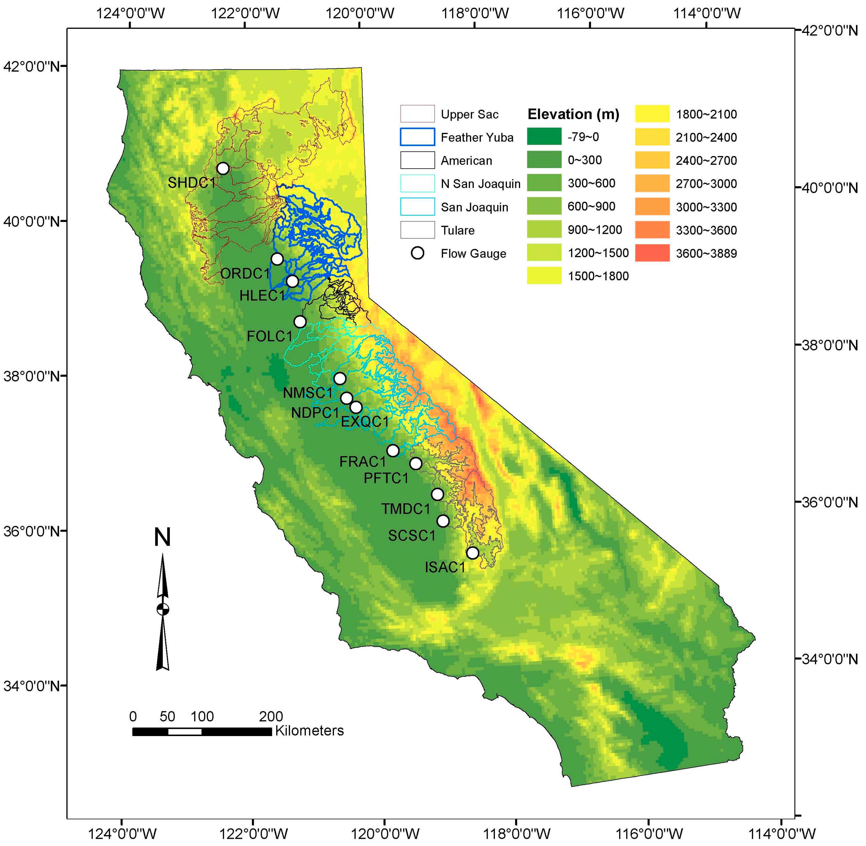
2.1. Study Area and Dataset
2.2. Study Indices
2.3. Trend Analysis
2.4. Distribution Pattern
3. Results
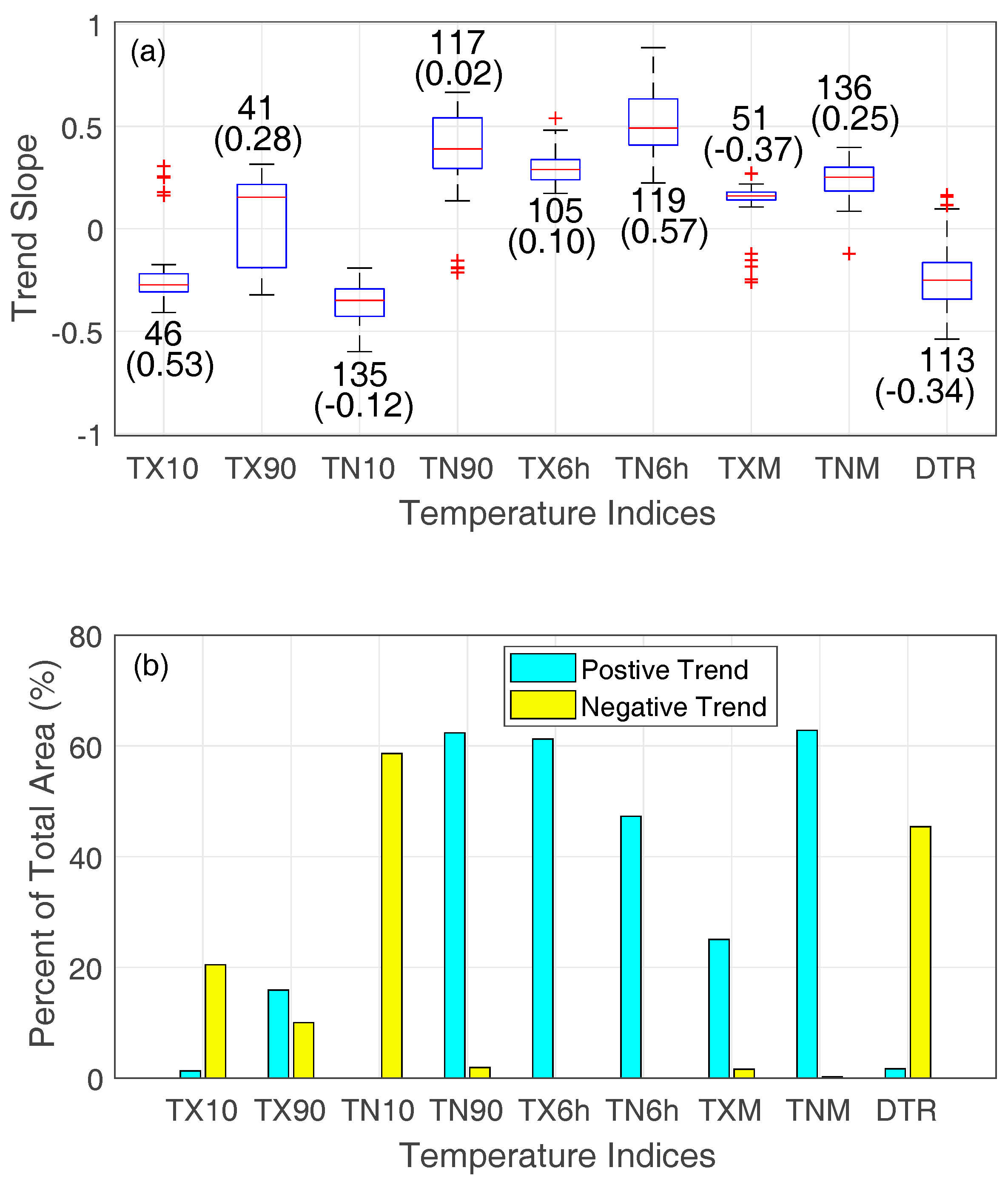
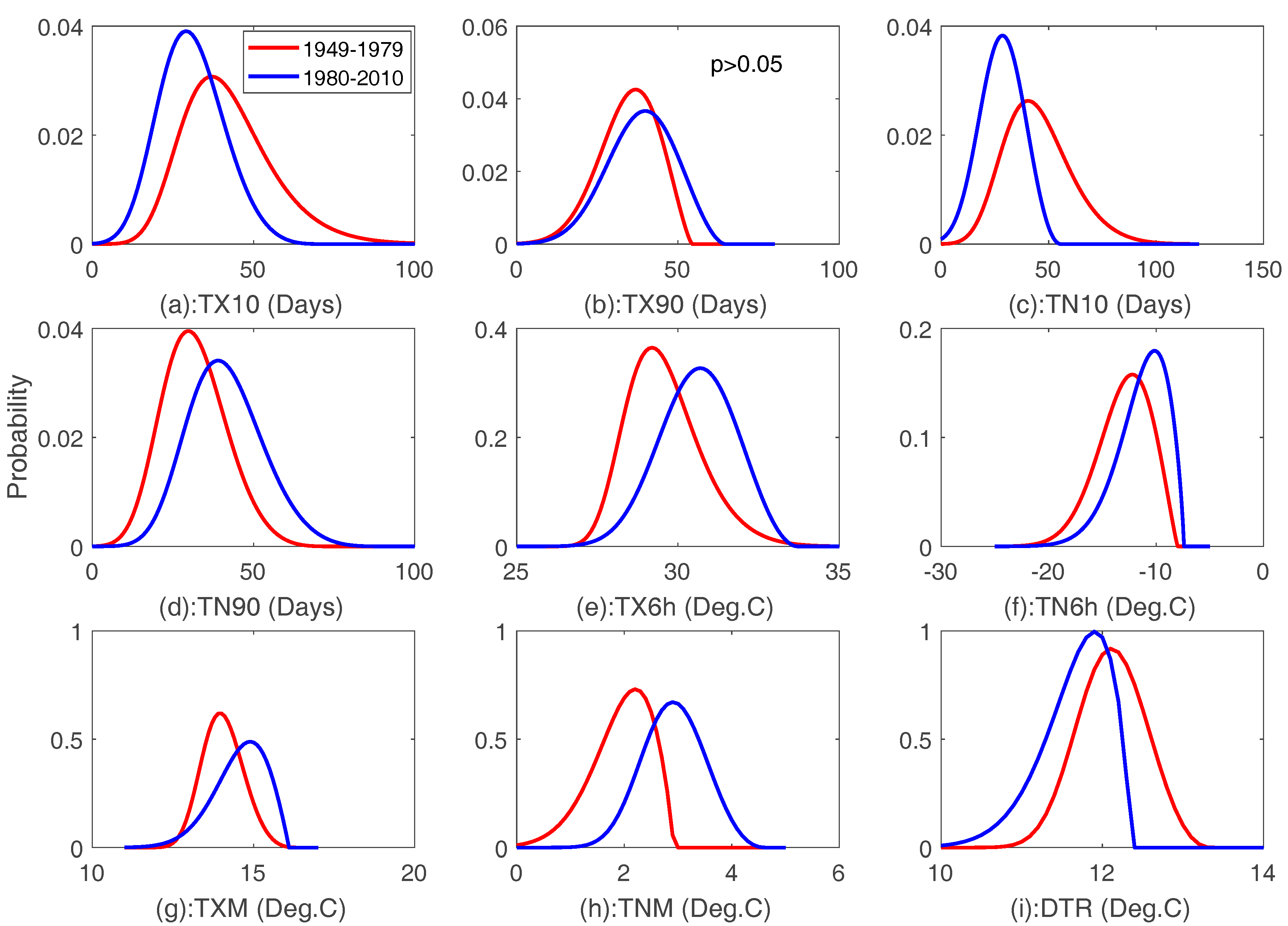
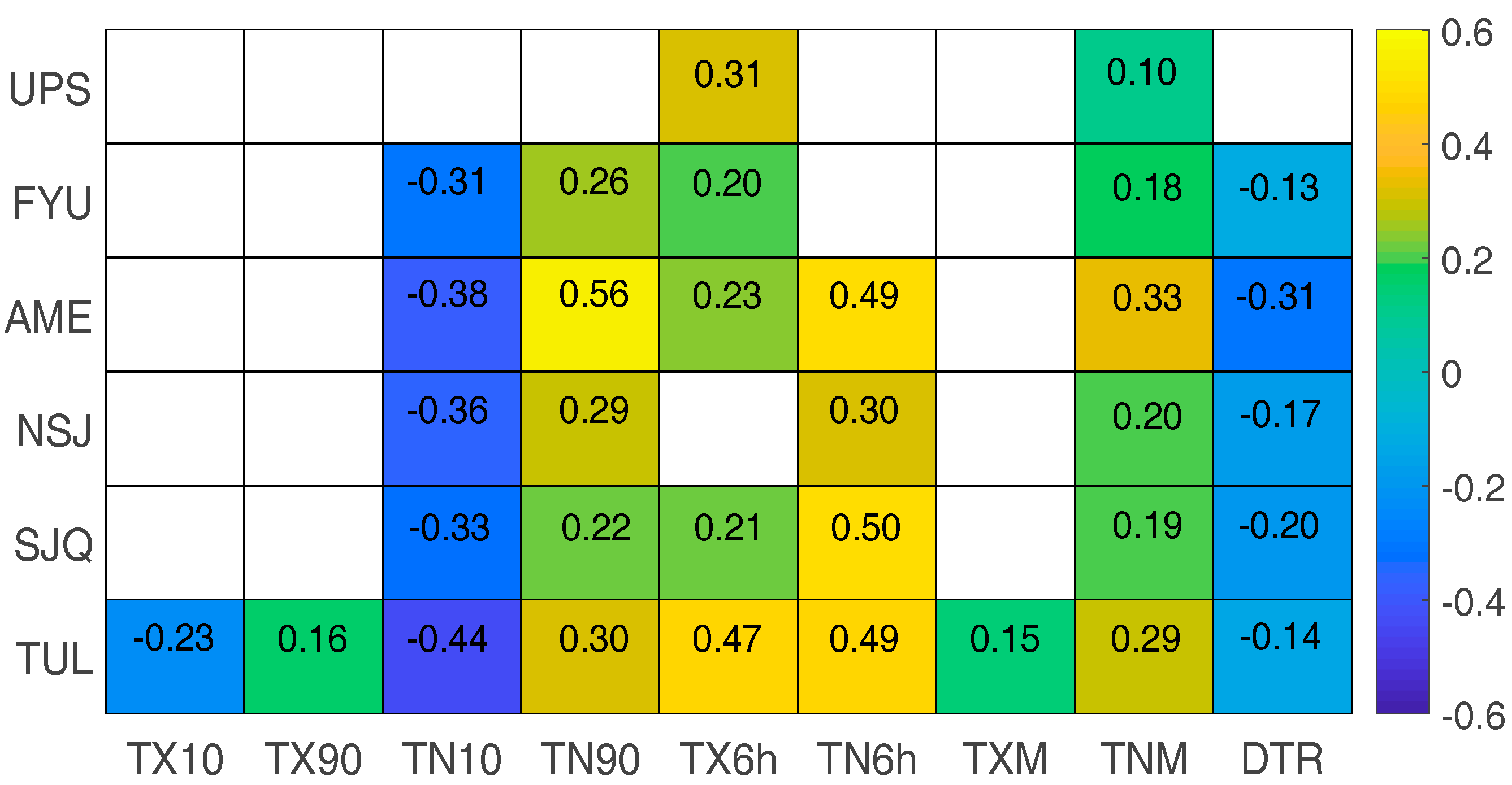
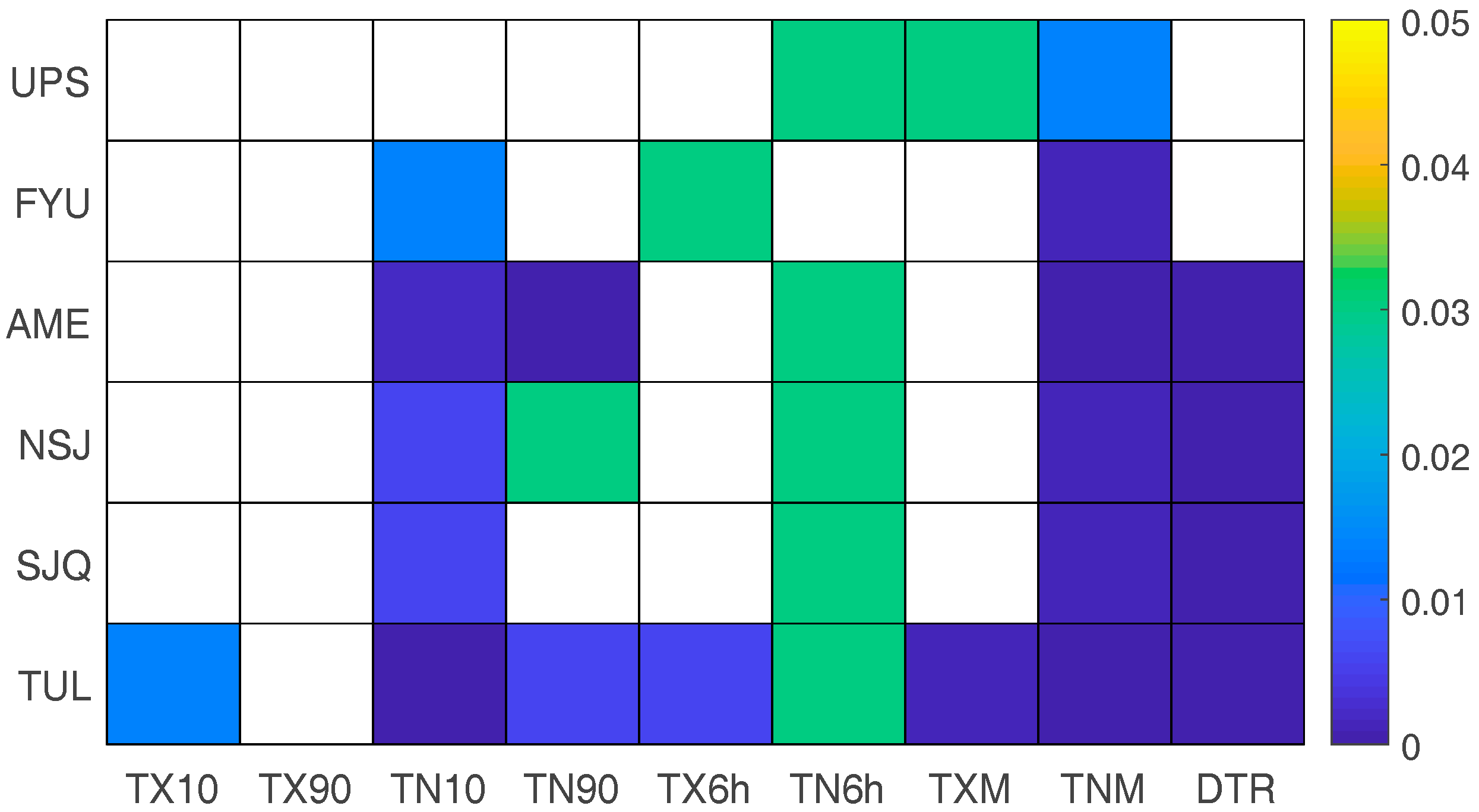
3.1. Temperature Indices
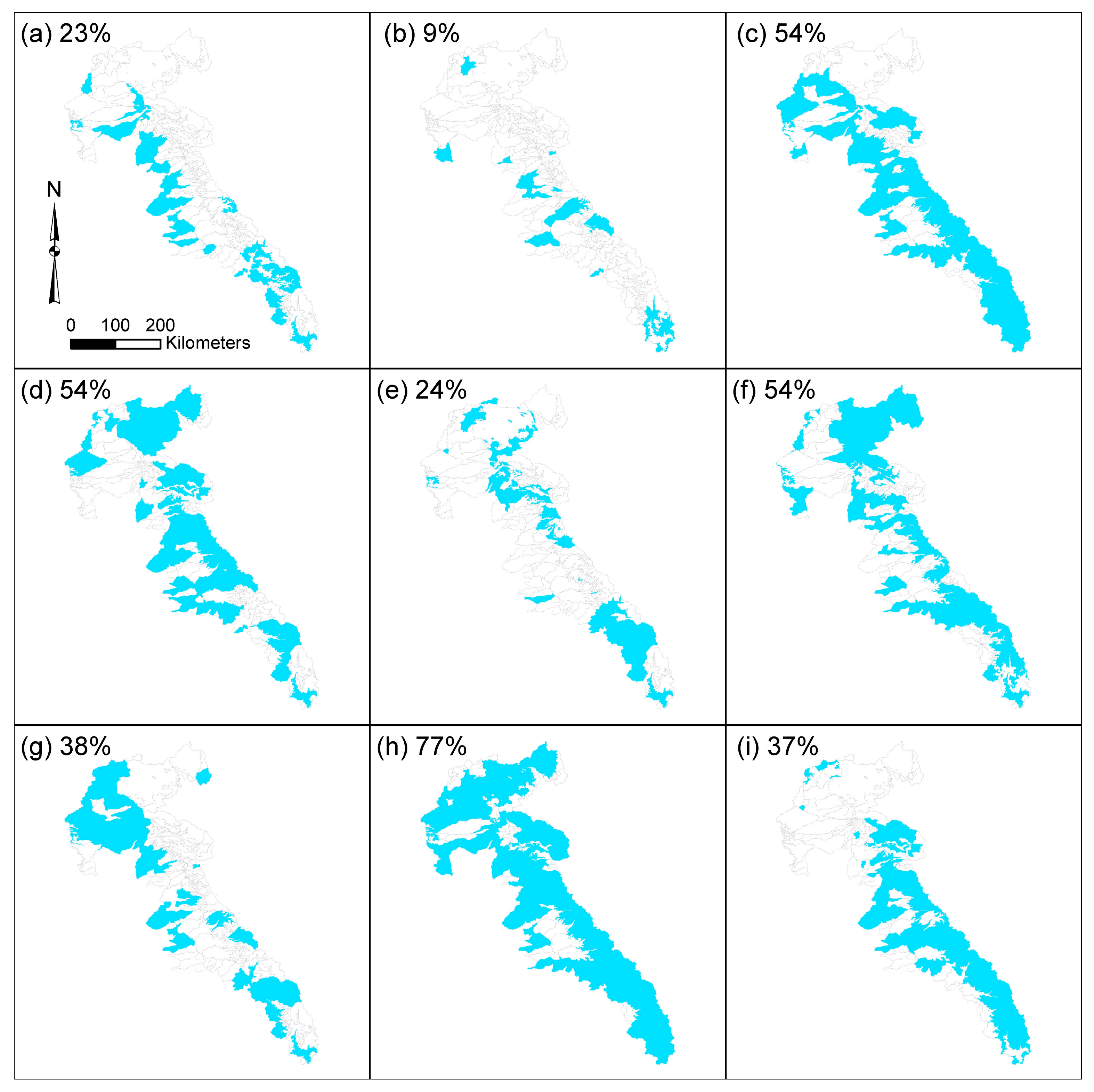
3.2. Precipitaiton Indices
3.3. Runoff Indices
4. Summary and Discussions
4.1. Temperature Indices
4.2. Precipitation Indices
4.3. Runoff Indices
4.4. Implications of This Study
5. Conclusions
Acknowledgments
Author Contributions
Conflicts of Interest
Appendix A


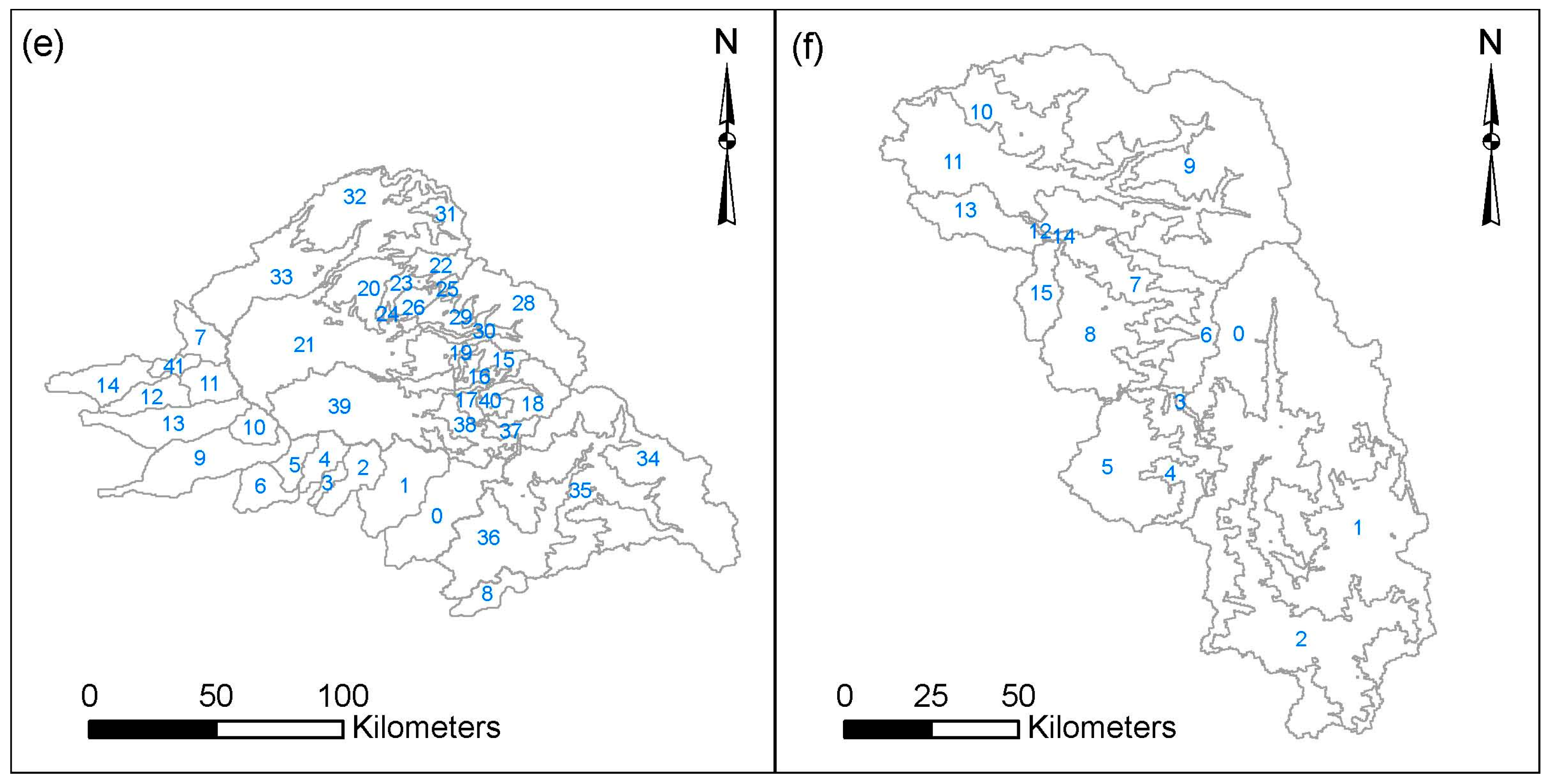
| No. | ID | Description | Elevation (m) | Area (km2) |
|---|---|---|---|---|
| 0 | SHDC1LOF | Sacramento River-Shasta Lake | 579 | 1126 |
| 1 | WHSC1HOF | Whiskeytown Dam | 1067 | 512 |
| 2 | HKCC1HOF | Big Chico Creek-Chico | 950 | 184 |
| 3 | EPRC1HOF | Little Stony Creek-East Park Reservoir | 549 | 251 |
| 4 | VWBC1LOF | Sacramento River-Vina Woodson Bridge | 347 | 586 |
| 5 | ORFC1LOF | Sacramento River-Ord Ferry | 107 | 1562 |
| 6 | RDGC1LOF | Clear Creek Near Igoca | 243 | 72 |
| 7 | BDBC1LOF | Sacramento River-Bend Bridge | 243 | 1267 |
| 8 | TCRC1HUF | Thomes Creek-Paskenta Upper | 1723 | 177 |
| 9 | TCRC1HLF | Thomes Creek-Paskenta Lower | 1112 | 343 |
| 10 | EDCC1HUF | Elder Creek-Paskenta Upper | 1670 | 35 |
| 11 | EDCC1HLF | Elder Creek-Paskenta Lower | 677 | 201 |
| 12 | COTC1HUF | Battle Creek-Cottonwood Upper | 1790 | 302 |
| 13 | COTC1HLF | Battle Creek-Cottonwood Lower | 973 | 612 |
| 14 | CWAC1HUF | Cottonwood Creek-Cottonwood Upper | 1676 | 166 |
| 15 | CWAC1HLF | Cottonwood Creek-Cottonwood Lower | 480 | 2207 |
| 16 | CWCC1HUF | Cow Creek-Millville Upper | 1676 | 87 |
| 17 | CWCC1HLF | Cow Creek-Millville Lower | 480 | 1001 |
| 18 | DLTC1HUF | Sacramento River-Delta Upper | 1783 | 283 |
| 19 | DLTC1HLF | Sacramento River-Delta Lower | 1052 | 805 |
| 20 | PITC1LUF | Pit River-Montgomery Creek Upper | 1798 | 1893 |
| 21 | PITC1LLF | Pit River-Montgomery Creek Lower | 1311 | 7121 |
| 22 | CNBC1LUF | Pit River-Canby Upper | 1890 | 637 |
| 23 | CNBC1LLF | Pit River-Canby Lower | 1496 | 2395 |
| 24 | PLYC1HUF | Sout Fork Pit River-Likely Upper | 2151 | 500 |
| 25 | PLYC1HLF | Sout Fork Pit River-Likely Lower | 1585 | 133 |
| 26 | BLBC1LUF | Stony Creek-Black Butte Reservoir Upper | 1685 | 79 |
| 27 | BLBC1LLF | Stony Creek-Black Butte Reservoir Lower | 590 | 1048 |
| 28 | SGEC1LUF | Stony Creek-Stony Gorge Reservoir Upper | 1681 | 62 |
| 29 | SGEC1LLF | Stony Creek-Stony Gorge Reservoir Lower | 541 | 457 |
| 30 | BKCC1HUF | Butte Creek Near Chico Upper | 1680 | 105 |
| 31 | BKCC1HLF | Butte Creek Near Chico Lower | 819 | 271 |
| 32 | TEHC1LUF | Sacramento River-Tehama Bridge Upper | 1722 | 27 |
| 33 | TEHC1LLF | Sacramento River-Tehama Bridge Lower | 347 | 1310 |
| 34 | DCVC1HUF | Deer Creek-Vina Upper | 1680 | 181 |
| 35 | DCVC1HLF | Deer Creek-Vina Lower | 819 | 351 |
| 36 | MLMC1HUF | Mill Creek-Los Molinos Upper | 1722 | 114 |
| 37 | MLMC1HLF | Mill Creek-Los Molinos Lower | 792 | 221 |
| 38 | MSSC1LLF | Mccloud River-Shasta Lake Lower | 1722 | 69 |
| 39 | MSSC1LUF | Mccloud River-Shasta Lake Upper | 1067 | 560 |
| 40 | MMCC1HLF | Mccloud River-Mccloud Lower | 1250 | 577 |
| 41 | MMCC1HUF | Mccloud River-Mccloud Upper | 1798 | 339 |
| No. | ID | Description | Elevation (m) | Area (km2) |
|---|---|---|---|---|
| 0 | DCWC1HOF | Wheatland Dry Creek | 222 | 256 |
| 1 | HCTC1HOF | South Fork Honcut Creek Nr Bangor | 514 | 78 |
| 2 | YUBC1LOF | Feather River-Yuba City | 59 | 763 |
| 3 | NBBC1LUF | North Fork Yuba River-New Bullards Bar Reservoir Upper | 1692 | 159 |
| 4 | NBBC1LLF | North Fork Yuba River-New Bullards Bar Reservoir Lower | 1063 | 453 |
| 5 | GYRC1HUF | North Yuba River Below Goodyears Bar Upper | 1920 | 442 |
| 6 | GYRC1HLF | North Yuba River Below Goodyears Bar Lower | 1280 | 198 |
| 7 | ORDC1LUF | Feather River-Lake Oroville Upper | 1676 | 199 |
| 8 | ORDC1LLF | Feather River-Lake Oroville Lower | 815 | 1047 |
| 9 | MRMC1LUF | Merrimac Middle Fork Feather Upper | 1745 | 731 |
| 10 | MRMC1LLF | Merrimac Middle Fork Feather Lower | 1347 | 487 |
| 11 | WBGC1HUF | West Branch Feather River- Magalia Upper | 1750 | 113 |
| 12 | WBGC1HLF | West Branch Feather River- Magalia Lower | 1062 | 156 |
| 13 | MFTC1HUF | Middle Fork Feather River-Portola Upper | 1849 | 1127 |
| 14 | MFTC1HLF | Middle Fork Feather River-Portola Lower | 1521 | 376 |
| 15 | IIFC1HUF | Indian Falls Indian Creek Upper | 1810 | 1476 |
| 16 | IIFC1HLF | Indian Falls Indian Creek Lower | 1200 | 416 |
| 17 | PLLC1HUF | North Fork Feather River-Prattville Upper | 1788 | 1006 |
| 18 | PLLC1HLF | North Fork Feather River-Prattville Lower | 1418 | 251 |
| 19 | CFWC1LOF | Bear River-Camp Far West Reservoir | 526 | 451 |
| 20 | ROLC1HLF | Bear River-Rollins Lake Lower | 980 | 253 |
| 21 | ROLC1HUF | Bear River-Rollins Lake Upper | 1608 | 13 |
| 22 | MRYC1LOF | Marysville Yuba | 137 | 187 |
| 23 | DMCC1HOF | Dry Creek-Merle Collins Reservoir | 671 | 183 |
| 24 | DCSC1HOF | Deer Creek-Smartsville | 693 | 170 |
| 25 | JKRC1HOF | Middle Fork Yuba River-Jackson Meadows Reservoir | 2088 | 96 |
| 26 | OURC1LLF | Middle Fork Yuba River-Our House Lower | 913 | 159 |
| 27 | OURC1LUF | Middle Fork Yuba River-Our House Upper | 1813 | 115 |
| 28 | BWKC1HOF | Canyon Creek-Bowman Reservoir | 2027 | 69 |
| 29 | FOCC1HOF | Fordyce Creek-Fordyce Lake | 2217 | 81 |
| 30 | SUAC1LOF | South Fork Yuba River-Lake Spaulding | 2027 | 221 |
| 31 | JNSC1LLF | South Fork Yuba River-Jones Bar Lower | 1052 | 305 |
| 32 | JNSC1LUF | South Fork Yuba River-Jones Bar Upper | 1753 | 113 |
| 33 | HLEC1LOF | Yuba River-Englebright Reservoir | 640 | 425 |
| 34 | PLGC1LLF | North Fork Feather River At Pulga Lower | 1092 | 626 |
| 35 | PLGC1LUF | North Fork Feather River At Pulga Upper | 1745 | 492 |
| 36 | SCBC1HLF | Spanish Creek-Keddie Lower | 1280 | 306 |
| 37 | SCBC1HUF | Spanish Creek-Keddie Upper | 1781 | 165 |
| 38 | NFEC1LLF | North Fork Feather River-East Branch Lower | 1195 | 188 |
| 39 | NFEC1LUF | North Fork Feather River-East Branch Upper | 1676 | 73 |
| No. | ID | Description | Elevation (m) | Area (km2) |
|---|---|---|---|---|
| 0 | FMDC1HOF | French Meadows Reservoir Near Foresthill | 1920 | 147 |
| 1 | FOLC1LOF | American River-Folsom Lake | 442 | 1016 |
| 2 | CBAC1LLF | South Fork American River-Chili Bar Reservoir Lower | 975 | 461 |
| 3 | CBAC1LUF | South Fork American River-Chili Bar Reservoir Upper | 1707 | 138 |
| 4 | UNVC1HLF | Union Valley Reservoir Lower | 1448 | 22 |
| 5 | UNVC1HUF | Union Valley Reservoir Upper | 1905 | 194 |
| 6 | RRGC1HOF | South Fork Rubicon River Below Gerle Creek | 1829 | 101 |
| 7 | SVCC1LLF | Silver Creek-Camino Reservoir Lower | 1402 | 81 |
| 8 | SVCC1LUF | Silver Creek-Camino Reservoir Upper | 1615 | 72 |
| 9 | MFAC1LLF | Foresthill Middle Fork American River Lower | 1097 | 106 |
| 10 | MFAC1LUF | Foresthill Middle Fork American River Upper | 1707 | 55 |
| 11 | RUFC1LLF | Rubicon River Near Foresthill Upper | 1250 | 274 |
| 12 | RUFC1LUF | Rubicon River Near Foresthill Lower | 1646 | 118 |
| 13 | HLLC1LLF | Rubicon River-Hell Hole Reservoir Lower | 1432 | 12 |
| 14 | HLLC1LUF | Rubicon River-Hell Hole Reservoir Upper | 2057 | 195 |
| 15 | ICHC1HOF | South Fork Silver Creek-Ice House Reservoir | 2088 | 70 |
| 16 | LNLC1HOF | Loon Lake | 1951 | 20 |
| 17 | RBBC1HOF | Rubicon River-Rockbound Lake | 2331 | 84 |
| 18 | NMFC1HLF | North Fork Of Middle Fork American River-Foresthill Lower | 1250 | 148 |
| 19 | NMFC1HUF | North Fork Of Middle Fork American River-Foresthill Upper | 1646 | 80 |
| 20 | NFDC1HLF | North Fork American River-North Fork Dam Lower | 1100 | 552 |
| 21 | NFDC1HUF | North Fork American River-North Fork Dam Upper | 1900 | 324 |
| 22 | AKYC1HLF | South Fork American River Near Kyburz Lower | 1371 | 20 |
| 23 | AKYC1HUF | South Fork American River Near Kyburz Upper | 2149 | 474 |
| No. | ID | Description | Elevation (m) | Area (km2) |
|---|---|---|---|---|
| 0 | MHBC1LOF | Cosumnes River-Michigan Bar | 457 | 573 |
| 1 | MCNC1LOF | Cosumnes River-Mcconnell | 61 | 486 |
| 2 | THTC1LOF | Mokelumne River-Benson Ferry | 530 | 829 |
| 3 | NHGC1HOF | Calaveras River-New Hogan Reservoir | 580 | 127 |
| 4 | FRGC1HOF | Littlejohns Creek-Farmington Reservoir | 122 | 497 |
| 5 | SOSC1HUF | Middle Fork Cosumnes River Nearr Somerset Upper | 1744 | 104 |
| 6 | SOSC1HLF | Middle Fork Cosumnes River Nearr Somerse Lower | 1196 | 170 |
| 7 | EDOC1HUF | North Fork Cosumnes River Nearr El Dorado Upper | 1745 | 115 |
| 8 | EDOC1HLF | North Fork Cosumnes River Nearr El Dorado Lower | 1013 | 409 |
| 9 | MSGC1LOF | Mormon Slough-Bellota | 122 | 276 |
| 10 | CMPC1HLF | Mokelumne River-Pardee Reservoir Lower | 1052 | 666 |
| 11 | CMPC1HUF | Mokelumne River-Pardee Reservoir Upper | 2179 | 814 |
| No. | ID | Description | Elevation (m) | Area (km2) |
|---|---|---|---|---|
| 0 | HIDC1HOF | Fresno River-Hensley Lake | 732 | 604 |
| 1 | BHNC1HOF | Chowchilla River-Buchanan Reservoir | 478 | 602 |
| 2 | MPAC1HOF | Mariposa Creek-Mariposa Reservoir | 550 | 274 |
| 3 | OWCC1HOF | Owens Creek-Owens Reservoir | 366 | 66 |
| 4 | BCKC1HOF | Bear Creek-Bear Reservoir | 442 | 184 |
| 5 | BNCC1HOF | Burns Creek-Burns Creek Reservoir | 283 | 189 |
| 6 | MEEC1LOF | Mckee Rd Bear Ck | 98 | 243 |
| 7 | KNFC1LOF | Stanislaus R Blo Goodwin Dam | 317 | 195 |
| 8 | LTDC1HOF | Friant Little Dry Ck | 282 | 181 |
| 9 | STVC1LOF | Merced River-Stevenson (Stvc1) | 107 | 154 |
| 10 | DSNC1HOF | Snelling Dry Ck | 230 | 187 |
| 11 | DRYC1HOF | Dry Creek At Crabtree Road | 300 | 228 |
| 12 | DCMC1LOF | Modesto Dry Ck | 300 | 282 |
| 13 | MDSC1LOF | Tuolumne River-Modesto (Mdsc1) | 35 | 128 |
| 14 | RIPC1LOF | Ripon Stanislaus | 61 | 154 |
| 15 | POHC1LUF | Merced River-Yosemite At Pohono Bridge Upper | 2500 | 161 |
| 16 | POHC1LMF | Merced River-Yosemite At Pohono Bridge Middle | 2100 | 176 |
| 17 | POHC1LLF | Merced River-Yosemite At Pohono Bridge Lower | 890 | 22 |
| 18 | HPIC1HUF | Happy Isles Merced River Upper | 2720 | 338 |
| 19 | NDPC1LUF | Tuolumne River-New Don Pedro Reservoir Upper | 2500 | 45 |
| 20 | NDPC1LMF | Tuolumne River-New Don Pedro Reservoir Middle | 2100 | 656 |
| 21 | NDPC1LLF | Tuolumne River-New Don Pedro Reservoir Lower | 900 | 1560 |
| 22 | CHVC1HUF | Cherry Creek-Cherry Lake Upper | 2650 | 171 |
| 23 | CHVC1HMF | Cherry Creek-Cherry Lake Middle | 2000 | 117 |
| 24 | CHVC1HLF | Cherry Creek-Cherry Lake Lower | 1450 | 12 |
| 25 | LNRC1HUF | Eleanor Creek-Lake Eleanor Upper | 2438 | 40 |
| 26 | LNRC1HMF | Eleanor Creek-Lake Eleanor Middle | 2000 | 150 |
| 27 | LNRC1HLF | Eleanor Creek-Lake Eleanor Lower | 1460 | 10 |
| 28 | HETC1HUF | Tuolumne River-Hetch Hetchy Reservoir Upper | 2819 | 228 |
| 29 | HETC1HMF | Tuolumne River-Hetch Hetchy Reservoir Middle | 2126 | 148 |
| 30 | HETC1HLF | Tuolumne River-Hetch Hetchy Reservoir Lower | 1280 | 24 |
| 31 | NMSC1HUF | Stanislaus River-New Melones Reservoir Upper | 2682 | 365 |
| 32 | NMSC1HMF | Stanislaus River-New Melones Reservoir Middle | 1966 | 621 |
| 33 | NMSC1HLF | Stanislaus River-New Melones Reservoir Lower | 884 | 840 |
| 34 | FRAC1HUF | San Joaquin River-Millerton Reservoir Upper | 2770 | 1803 |
| 35 | FRAC1HMF | San Joaquin River-Millerton Reservoir Middle | 2100 | 1342 |
| 36 | FRAC1HLF | San Joaquin River-Millerton Reservoir Lower | 890 | 1048 |
| 37 | EXQC1LUF | Merced River-Exchequer Reservoir Upper | 2500 | 128 |
| 38 | EXQC1LMF | Merced River-Exchequer Reservoir Middle | 2100 | 440 |
| 39 | EXQC1LLF | Merced River-Exchequer Reservoir Lower | 900 | 1265 |
| 40 | HPIC1HMF | Happy Isles Merced River Middle | 2000 | 125 |
| 41 | OBBC1LOF | Stanislaus River-Orange Blossom | 107 | 90 |
| No. | ID | Description | Elevation (m) | Area (km2) |
|---|---|---|---|---|
| 0 | ISAC1HUF | Kern River-Lake Isabella Upper | 2591 | 54 |
| 1 | ISAC1HMF | Kern River-Lake Isabella Middle | 1905 | 840 |
| 2 | ISAC1HLF | Kern River-Lake Isabella Lower | 1143 | 893 |
| 3 | SCSC1HUF | Tule River-Lake Success Upper | 2621 | 50 |
| 4 | SCSC1HMF | Tule River-Lake Success Middle | 1905 | 300 |
| 5 | SCSC1HLF | Tule River-Lake Success Lower | 793 | 649 |
| 6 | TMDC1HUF | Kaweah River-Lake Kaweah Upper | 2591 | 51 |
| 7 | TMDC1HMF | Kaweah River-Lake Kaweah Middle | 1905 | 51 |
| 8 | TMDC1HLF | Kaweah River-Lake Kaweah Lower | 1143 | 262 |
| 9 | PFTC1HUF | Kings River-Pine Flat Reservoir Upper | 3048 | 2095 |
| 10 | PFTC1HMF | Kings River-Pine Flat Reservoir Middle | 2042 | 1028 |
| 11 | PFTC1HLF | Kings River-Pine Flat Reservoir Lower | 890 | 830 |
| 12 | MLPC1HUF | Piedra Mill Creek Upper | 1685 | 13 |
| 13 | MLPC1HLF | Piedra Mill Creek Lower | 747 | 312 |
| 14 | DLMC1HUF | Lemoncove Dry Creek Upper | 1752 | 6 |
| 15 | DLMC1HLF | Lemoncove Dry Creek Lower | 762 | 188 |
References
- Easterling, D.R.; Meehl, G.A.; Parmesan, C.; Changnon, S.A.; Karl, T.R.; Mearns, L.O. Climate extremes: Observations, modeling, and impacts. Science 2000, 289, 2068–2074. [Google Scholar] [CrossRef] [PubMed]
- Changnon, S.A.; Pielke, R.A., Jr.; Changnon, D.; Sylves, R.T.; Pulwarty, R. Human factors explain the increased losses from weather and climate extremes. Bull. Am. Meteorol. Soc. 2000, 81, 437–442. [Google Scholar] [CrossRef]
- Bouwer, L.M. Have disaster losses increased due to anthropogenic climate change? Bull. Am. Meteorol. Soc. 2011, 92, 39–46. [Google Scholar] [CrossRef]
- Nutter, F.W. Global climate change: Why U.S. Insurers care. In Weather and Climate Extremes; Springer: Dordrecht, The Netherlands, 1999; pp. 45–49. [Google Scholar]
- Su, B.; Jiang, T.; Jin, W. Recent trends in observed temperature and precipitation extremes in the Yangtze River Basin, China. Theor. Appl. Climatol. 2006, 83, 139–151. [Google Scholar] [CrossRef]
- Mora, C.; Dousset, B.; Caldwell, I.R.; Powell, F.E.; Geronimo, R.C.; Bielecki, C.R.; Counsell, C.W.; Dietrich, B.S.; Johnston, E.T.; Louis, L.V. Global risk of deadly heat. Nat. Clim. Chang. 2017, 7, 501–506. [Google Scholar] [CrossRef]
- AghaKouchak, A.; Cheng, L.; Mazdiyasni, O.; Farahmand, A. Global warming and changes in risk of concurrent climate extremes: Insights from the 2014 California drought. Geophys. Res. Lett. 2014, 41, 8847–8852. [Google Scholar] [CrossRef]
- Yoon, J.-H.; Wang, S.S.; Gillies, R.R.; Kravitz, B.; Hipps, L.; Rasch, P.J. Increasing water cycle extremes in California and in relation to ENSO cycle under global warming. Nat. Commun. 2015, 6, 8657. [Google Scholar] [CrossRef] [PubMed]
- Berg, N.; Hall, A. Increased interannual precipitation extremes over California under climate change. J. Clim. 2015, 28, 6324–6334. [Google Scholar] [CrossRef]
- Alexander, L.; Zhang, X.; Peterson, T.; Caesar, J.; Gleason, B.; Tank, A.K.; Haylock, M.; Collins, D.; Trewin, B.; Rahimzadeh, F. Global observed changes in daily climate extremes of temperature and precipitation. J. Geophys. Res. Atmos. 2006, 111. [Google Scholar] [CrossRef] [Green Version]
- He, M.; Gautam, M. Variability and trends in precipitation, temperature and drought indices in the State of California. Hydrology 2016, 3, 14. [Google Scholar] [CrossRef]
- Peterson, T.C.; Taylor, M.A.; Demeritte, R.; Duncombe, D.L.; Burton, S.; Thompson, F.; Porter, A.; Mercedes, M.; Villegas, E.; Fils, R.S. Recent changes in climate extremes in the Caribbean region. J. Geophys. Res. Atmos. 2002, 107, 4601. [Google Scholar] [CrossRef]
- Easterling, D.R.; Evans, J.; Groisman, P.Y.; Karl, T.R.; Kunkel, K.E.; Ambenje, P. Observed variability and trends in extreme climate events: A brief review. Bull. Am. Meteorol. Soc. 2000, 81, 417–425. [Google Scholar] [CrossRef]
- Vincent, L.A.; Peterson, T.; Barros, V.; Marino, M.; Rusticucci, M.; Carrasco, G.; Ramirez, E.; Alves, L.; Ambrizzi, T.; Berlato, M. Observed trends in indices of daily temperature extremes in South America 1960–2000. J. Clim. 2005, 18, 5011–5023. [Google Scholar] [CrossRef]
- Haylock, M.R.; Peterson, T.; Alves, L.; Ambrizzi, T.; Anunciação, Y.; Baez, J.; Barros, V.; Berlato, M.; Bidegain, M.; Coronel, G. Trends in total and extreme South American rainfall in 1960–2000 and links with sea surface temperature. J. Clim. 2006, 19, 1490–1512. [Google Scholar] [CrossRef]
- Zhang, X.; Aguilar, E.; Sensoy, S.; Melkonyan, H.; Tagiyeva, U.; Ahmed, N.; Kutaladze, N.; Rahimzadeh, F.; Taghipour, A.; Hantosh, T. Trends in Middle East climate extreme indices from 1950 to 2003. J. Geophys. Res. Atmos. 2005, 110. [Google Scholar] [CrossRef]
- Aguilar, E.; Barry, A.A.; Brunet, M.; Ekang, L.; Fernandes, A.; Massoukina, M.; Mbah, J.; Mhanda, A.; Do Nascimento, D.; Peterson, T. Changes in temperature and precipitation extremes in western Central Africa, Guinea Conakry, and Zimbabwe, 1955–2006. J. Geophys. Res. Atmos. 2009, 114. [Google Scholar] [CrossRef]
- United States Census Bureau. 2010 Census Summary File 1. Available online: https://www.census.gov/2010census/data/ (accessed on 1 August 2017).
- Dettinger, M.D.; Ralph, F.M.; Das, T.; Neiman, P.J.; Cayan, D.R. Atmospheric rivers, floods and the water resources of California. Water 2011, 3, 445–478. [Google Scholar] [CrossRef]
- He, M.; Russo, M.; Anderson, M. Hydroclimatic characteristics of the 2012–2015 California drought from an operational perspective. Climate 2017, 5, 5. [Google Scholar] [CrossRef]
- Chung, F.; Kelly, K.; Guivetchi, K. Averting a California water crisis. J. Water Resour. Plan. Manag. 2002, 128, 237–239. [Google Scholar] [CrossRef]
- Pryor, S.; Howe, J.; Kunkel, K. How spatially coherent and statistically robust are temporal changes in extreme precipitation in the Contiguous USA? Int. J. Climatol. 2009, 29, 31–45. [Google Scholar] [CrossRef]
- Grundstein, A.; Dowd, J. Trends in extreme apparent temperatures over the United States, 1949–2010. J. Appl. Meteorol. Clim. 2011, 50, 1650–1653. [Google Scholar] [CrossRef]
- Grundstein, A. Evaluation of climate change over the continental United States using a moisture index. Clim. Chang. 2009, 93, 103–115. [Google Scholar] [CrossRef]
- Schwartz, M.D.; Ault, T.R.; Betancourt, J.L. Spring onset variations and trends in the continental United States: Past and regional assessment using temperature-based indices. Int. J. Climatol. 2013, 33, 2917–2922. [Google Scholar] [CrossRef]
- Bonfils, C.; Duffy, P.B.; Santer, B.D.; Wigley, T.M.; Lobell, D.B.; Phillips, T.J.; Doutriaux, C. Identification of external influences on temperatures in California. Clim. Chang. 2008, 87, 43–55. [Google Scholar] [CrossRef]
- Caroni, C.; Panagoulia, D.; Economou, P. Non-stationary modelling of extremes of precipitation and temperature over mountainous areas under climate change. In Proceedings of the International Conference in Current Topics on Risk Analysis, Barcelona, Spain, 26–29 May 2015; pp. 203–209. [Google Scholar]
- Panagoulia, D.; Economou, P.; Caroni, C. Stationary and nonstationary generalized extreme value modelling of extreme precipitation over a mountainous area under climate change. Environmetrics 2014, 25, 29–43. [Google Scholar] [CrossRef]
- Daly, C. Climate division normals derived from topographically-sensitive climate grids. In Proceedings of the 13th AMS Conference on Applied Climatology, Portland, OR, USA, 13–16 May 2002; pp. 177–180. [Google Scholar]
- Smith, M.B.; Laurine, D.P.; Koren, V.I.; Reed, S.M.; Zhang, Z. Hydrologic model calibration in the National Weather Service. In Calibration of Watershed Models; Wiley: Washington, DC, USA, 2003; pp. 133–152. [Google Scholar]
- Peterson, T.; Folland, C.; Gruza, G.; Hogg, W.; Mokssit, A.; Plummer, N. Report on the Activities of the Working Group on Climate Change Detection and Related Rapporteurs; World Meteorological Organization: Geneva, Switzerland, 2001. [Google Scholar]
- Wang, W.; Shao, Q.; Yang, T.; Peng, S.; Yu, Z.; Taylor, J.; Xing, W.; Zhao, C.; Sun, F. Changes in daily temperature and precipitation extremes in the Yellow River Basin, China. Stoch. Environ. Res. Risk Assess. 2013, 27, 401–421. [Google Scholar] [CrossRef]
- Vincent, L.; Aguilar, E.; Saindou, M.; Hassane, A.; Jumaux, G.; Roy, D.; Booneeady, P.; Virasami, R.; Randriamarolaza, L.; Faniriantsoa, F. Observed trends in indices of daily and extreme temperature and precipitation for the countries of the Western Indian Ocean, 1961–2008. J. Geophys. Res. Atmos. 2011, 116. [Google Scholar] [CrossRef]
- New, M.; Hewitson, B.; Stephenson, D.B.; Tsiga, A.; Kruger, A.; Manhique, A.; Gomez, B.; Coelho, C.A.; Masisi, D.N.; Kululanga, E. Evidence of trends in daily climate extremes over southern and west Africa. J. Geophys. Res. Atmos. 2006, 111. [Google Scholar] [CrossRef]
- Tank, A.K.; Peterson, T.; Quadir, D.; Dorji, S.; Zou, X.; Tang, H.; Santhosh, K.; Joshi, U.; Jaswal, A.; Kolli, R. Changes in daily temperature and precipitation extremes in central and south Asia. J. Geophys. Res. Atmos. 2006, 111. [Google Scholar] [CrossRef]
- California Department of Water Resources. Central Valley Flood Protection Plan 2017 Update. Available online: http://www.water.ca.gov/cvfmp/docs/2017/2017CVFPPUpdate-Final-20170828.pdf (accessed on 1 October 2017).
- Stewart, I.T.; Cayan, D.R.; Dettinger, M.D. Changes in snowmelt runoff timing in western North America under a business-as-usual climate change scenario. Clim. Chang. 2004, 62, 217–232. [Google Scholar] [CrossRef]
- Stewart, I.T.; Cayan, D.R.; Dettinger, M.D. Changes toward earlier streamflow timing across western North America. J. Clim. 2005, 18, 1136–1155. [Google Scholar] [CrossRef]
- Hirsch, R.M.; Helsel, D.; Cohn, T.; Gilroy, E. Statistical analysis of hydrologic data. Handb. Hydrol. 1993, 17, 11–55. [Google Scholar]
- Helsel, D.R.; Hirsch, R.M. Statistical Methods in Water Resources; Elsevier: Amsterdam, The Netherlands, 1992; Volume 49. [Google Scholar]
- Mann, H. Non-parametric tests against trend. Econometrica 1945, 13, 245–259. [Google Scholar] [CrossRef]
- Kendall, M.G. Rank Correlation Methods; Charles Griffin: London, UK, 1975. [Google Scholar]
- Yue, S.; Pilon, P.; Phinney, B.; Cavadias, G. The influence of autocorrelation on the ability to detect trend in hydrological series. Hydrol. Process. 2002, 16, 1807–1829. [Google Scholar] [CrossRef]
- Thiel, H. A rank-invariant method of linear and polynomial regression analysis, part 3. Proc. Koninalijke Ned. Akad. Weinenschatpen A 1950, 53, 1397–1412. [Google Scholar]
- Sen, P.K. Estimates of the regression coefficient based on Kendall’s tau. J. Am. Stat. Assoc. 1968, 63, 1379–1389. [Google Scholar] [CrossRef]
- Von Storch, H. Misuses of statistical analysis in climate research. In Analysis of Climate Variability; Springer: Berlin/Heidelberg, Germany, 1995; pp. 11–26. [Google Scholar]
- Douglas, E.; Vogel, R.; Kroll, C. Trends in floods and low flows in the United States: Impact of spatial correlation. J. Hydrol. 2000, 240, 90–105. [Google Scholar] [CrossRef]
- Hamed, K.H.; Rao, A.R. A modified Mann-Kendall trend test for autocorrelated data. J. Hydrol. 1998, 204, 182–196. [Google Scholar] [CrossRef]
- Yue, S.; Pilon, P.; Phinney, B. Canadian streamflow trend detection: Impacts of serial and cross-correlation. Hydrol. Sci. J. 2003, 48, 51–63. [Google Scholar] [CrossRef]
- Massey, F.J., Jr. The Kolmogorov-Smirnov test for goodness of fit. J. Am. Stat. Assoc. 1951, 46, 68–78. [Google Scholar] [CrossRef]
- Qin, N.; Chen, X.; Fu, G.; Zhai, J.; Xue, X. Precipitation and temperature trends for the southwest China: 1960–2007. Hydrol. Process. 2010, 24, 3733–3744. [Google Scholar] [CrossRef]
- Soro, G.E.; Noufé, D.; Goula Bi, T.A.; Shorohou, B. Trend analysis for extreme rainfall at sub-daily and daily timescales in Côte d’Ivoire. Climate 2016, 4, 37. [Google Scholar] [CrossRef]
- Attogouinon, A.A.; Lawin, A.E.; M’Po, Y.N.T.; Houngue, R. Extreme precipitation indices trend assessment over the upper Uueme River Valley (Benin). Hydrology 2017, 4, 36. [Google Scholar] [CrossRef]
- Regonda, S.K.; Rajagopalan, B.; Clark, M.; Pitlick, J. Seasonal cycle shifts in hydroclimatology over the western United States. J. Clim. 2005, 18, 372–384. [Google Scholar] [CrossRef]
- McCabe, G.J.; Clark, M.P. Trends and variability in snowmelt runoff in the western United States. J. Hydrometeorol. 2005, 6, 476–482. [Google Scholar] [CrossRef]
- Hidalgo, H.; Das, T.; Dettinger, M.; Cayan, D.; Pierce, D.; Barnett, T.; Bala, G.; Mirin, A.; Wood, A.; Bonfils, C. Detection and attribution of streamflow timing changes to climate change in the western United States. J. Clim. 2009, 22, 3838–3855. [Google Scholar] [CrossRef]
- Dudley, R.; Hodgkins, G.; McHale, M.; Kolian, M.; Renard, B. Trends in snowmelt-related streamflow timing in the Conterminous United States. J. Hydrol. 2017, 547, 208–221. [Google Scholar] [CrossRef]
- Burn, D.H. Climatic influences on streamflow timing in the headwaters of the Mackenzie River Basin. J. Hydrol. 2008, 352, 225–238. [Google Scholar] [CrossRef]
- Lins, H.F.; Slack, J.R. Streamflow trends in the United States. Geophys. Res. Lett. 1999, 26, 227–230. [Google Scholar] [CrossRef]
- Tamaddun, K.; Kalra, A.; Ahmad, S. Identification of streamflow changes across the Continental United States using variable record lengths. Hydrology 2016, 3, 24. [Google Scholar] [CrossRef]
- Anderson, E.A. National Weather Service River Forecast System—Snow Accumulation and Ablation Model; Technical Memorandum NWS HYDRO-17, November 1973; NOAA: Washington, DC, USA, 1973; p. 217.
- Mote, P.W.; Hamlet, A.F.; Clark, M.P.; Lettenmaier, D.P. Declining mountain snowpack in western North America. Bull. Am. Meteorol. Soc. 2005, 86, 39–49. [Google Scholar] [CrossRef]
- Mote, P.W. Trends in snow water equivalent in the Pacific Northwest and their climatic causes. Geophys. Res. Lett. 2003, 30. [Google Scholar] [CrossRef]
- Kapnick, S.; Hall, A. Observed climate–snowpack relationships in California and their implications for the future. J. Clim. 2010, 23, 3446–3456. [Google Scholar] [CrossRef]
- Sun, F.; Hall, A.; Schwartz, M.; Walton, D.B.; Berg, N. Twenty-first-century snowfall and snowpack changes over the southern California mountains. J. Clim. 2016, 29, 91–110. [Google Scholar] [CrossRef]
- Painter, T.; Berisford, D.; Boardman, J.; Bormann, K.; Deems, J.; Gehrke, F.; Hedrick, A.; Joyce, M.; Laidlaw, R.; Marks, D. The airborne snow observatory: Scanning lidar and imaging spectrometer fusion for mapping snow water equivalent and snow albedo. Remote Sens. Environ. 2016, 184, 139–152. [Google Scholar] [CrossRef]
- Seidel, F.C.; Rittger, K.; Skiles, S.; Molotch, N.P.; Painter, T.H. Case study of spatial and temporal variability of snow cover, grain size, albedo and radiative forcing in the Sierra Nevada and rocky mountain snowpack derived from imaging spectroscopy. Cryosphere 2016, 10, 1229–1244. [Google Scholar] [CrossRef]
- Huning, L.S.; Margulis, S.A. Climatology of seasonal snowfall accumulation across the Sierra Nevada (USA): Accumulation rates, distributions, and variability. Water Resour. Res. 2017. [Google Scholar] [CrossRef]
- Sturm, M. White water: Fifty years of snow research in wrr and the outlook for the future. Water Resour. Res. 2015, 51, 4948–4965. [Google Scholar] [CrossRef]
- Cayan, D.R.; Maurer, E.P.; Dettinger, M.D.; Tyree, M.; Hayhoe, K. Climate change scenarios for the California region. Clim. Chang. 2008, 87, 21–42. [Google Scholar] [CrossRef]
- Dettinger, M.D. Projections and downscaling of 21st century temperatures, precipitation, radiative fluxes and winds for the southwestern US, with focus on Lake Tahoe. Clim. Chang. 2013, 116, 17–33. [Google Scholar] [CrossRef]
- Scherer, M.; Diffenbaugh, N.S. Transient twenty-first century changes in daily-scale temperature extremes in the United States. Clim. Dyn. 2014, 42, 1383–1404. [Google Scholar] [CrossRef]
- Das, T.; Dettinger, M.D.; Cayan, D.R.; Hidalgo, H.G. Potential increase in floods in California’s Sierra Nevada under future climate projections. Clim. Chang. 2011, 109, 71–94. [Google Scholar] [CrossRef]
- Das, T.; Maurer, E.P.; Pierce, D.W.; Dettinger, M.D.; Cayan, D.R. Increases in flood magnitudes in California under warming climates. J. Hydrol. 2013, 501, 101–110. [Google Scholar] [CrossRef]
- Feng, S.; Hu, Q. Changes in winter snowfall/precipitation ratio in the Contiguous United States. J. Geophys. Res. Atmos. 2007, 112. [Google Scholar] [CrossRef]
- Coats, R. Climate change in the Tahoe basin: Regional trends, impacts and drivers. Clim. Chang. 2010, 102, 435–466. [Google Scholar] [CrossRef]
- Andrew, J.T.; Sauquet, E. Climate change impacts and water management adaptation in two mediterranean-climate watersheds: Learning from the Durance and Sacramento rivers. Water 2016, 9, 126. [Google Scholar] [CrossRef]

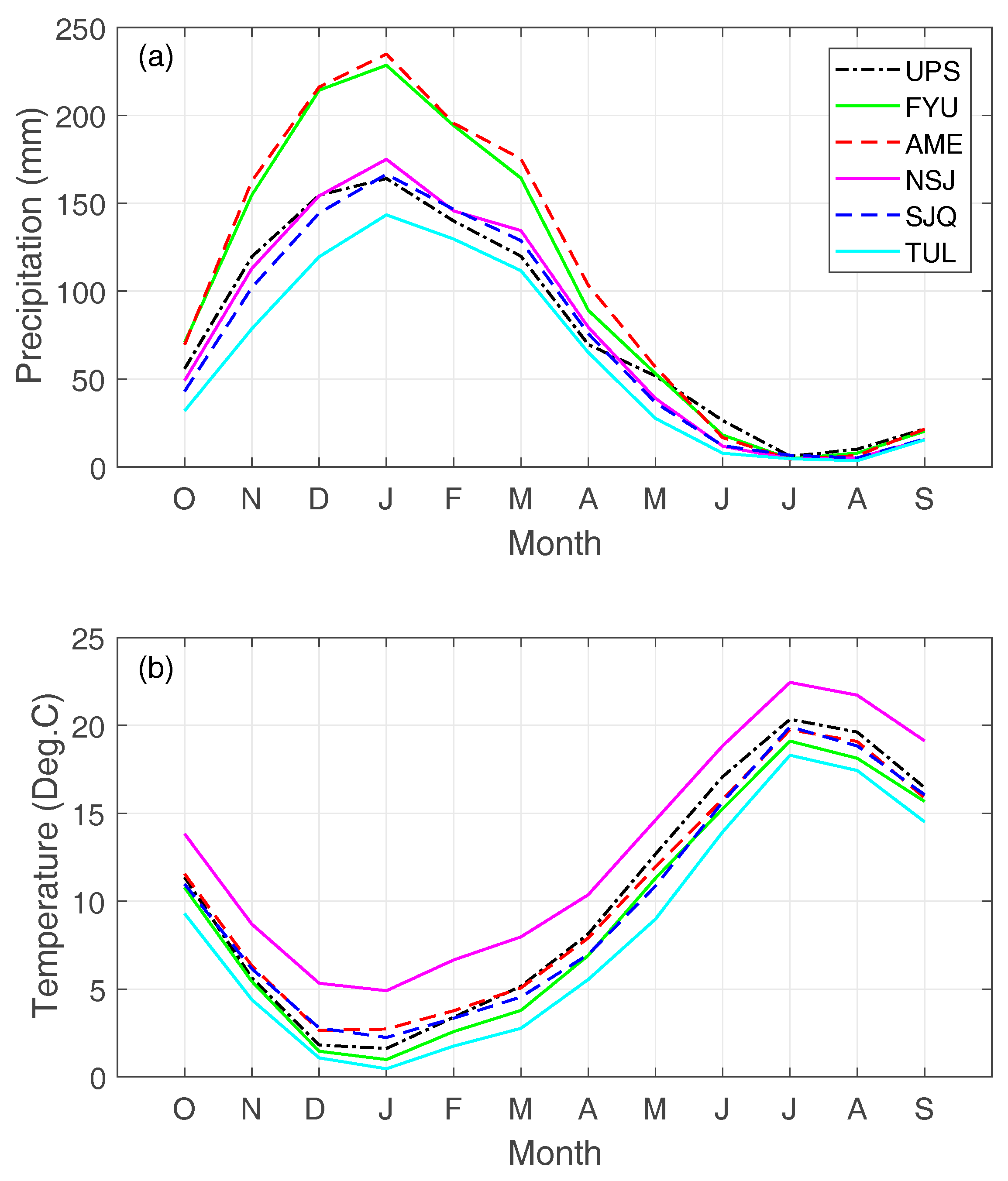


| Group Name | ID | Area (km2) | Annual Precipitation (mm) 1 | Annual Temperature (°C) 1 |
|---|---|---|---|---|
| Upper Sacramento | UPS | 30229 | 940 | 10.3 |
| Feather Yuba | FYU | 14425 | 1220 | 9.3 |
| American | AME | 4764 | 1264 | 10.2 |
| North San Joaquin | NSJ | 5066 | 927 | 12.9 |
| San Joaquin | SJQ | 15596 | 884 | 9.9 |
| Tulare | TUL | 7622 | 739 | 8.2 |
| Reservoir Name | ID | Reservoir Capacity (109 m3) | Drainage Area (km2) | Unimpaired Inflow | |||
|---|---|---|---|---|---|---|---|
| April–July 1 (AJ, 109 m3) | Annual 1 (A, 109 m3) | Ratio (AJ/A) | Record Period (Water Year) | ||||
| Shasta Lake | SHDC1 | 5.61 | 16630 | 2.24 | 7.38 | 0.30 | 1961–2010 |
| Lake Oroville | ORDC1 | 4.36 | 9352 | 1.96 | 5.19 | 0.38 | 1961–2010 |
| Englebright Reservoir | HLEC1 | 0.09 | 2836 | 1.16 | 2.73 | 0.42 | 1970–2010 |
| Folsom Lake | FOLC1 | 1.21 | 4856 | 1.48 | 3.32 | 0.45 | 1961–2010 |
| New Melones Reservoir | NMSC1 | 2.96 | 2341 | 0.84 | 1.44 | 0.58 | 1961–2010 |
| Don Pedro Reservoir | NDPC1 | 2.50 | 3970 | 1.49 | 2.38 | 0.63 | 1971–2010 |
| Lake McClure | EXQC1 | 1.26 | 2686 | 0.77 | 1.22 | 0.63 | 1961–2010 |
| Millerton Lake | FRAC1 | 0.64 | 4242 | 1.55 | 2.26 | 0.69 | 1961–2010 |
| Pine Flat Reservoir | PFTC1 | 1.23 | 4105 | 1.53 | 2.14 | 0.72 | 1961–2010 |
| Lake Kaweah | TMDC1 | 0.23 | 1436 | 0.36 | 0.56 | 0.64 | 1961–2010 |
| Lake Success | SCSC1 | 0.10 | 1006 | 0.08 | 0.18 | 0.44 | 1961–2010 |
| Lake Isabella | ISAC1 | 0.70 | 5309 | 0.57 | 0.90 | 0.63 | 1961–2010 |
| Variable | Index | Description | Unit |
|---|---|---|---|
| Temperature | TX6h | Annual maximum six-hour temperature | °C |
| TN6h | Annual minimum six-hour temperature | °C | |
| TXM | Annual mean of daily maximum temperature (TX6h) | °C | |
| TNM | Annual mean of daily minimum temperature (TN6h) | °C | |
| DTR | Annual mean of diurnal temperature range | °C | |
| TX10 | Cold days (with TX below 10th percentile temperature) | days | |
| TX90 | Warm days (with TX above 90th percentile temperature) | days | |
| TN10 | Cold nights (with TN below 10th percentile temperature) | days | |
| TN90 | Warm nights (with TN above 10th percentile temperature) | days | |
| Precipitation | R10 | Annual count of days with precipitation above 10 mm | days |
| R20 | Annual count of days with precipitation above 20 mm | days | |
| R6h | Annual maximum six-hour precipitation | mm | |
| R1D | Annual maximum daily precipitation | mm | |
| R3D | Annual maximum three-day precipitation | mm | |
| R5D | Annual maximum five-day precipitation | mm | |
| R95 | Annual count of precipitation above 95th percentile | mm | |
| R99 | Annual count of precipitation above 99th percentile | mm | |
| SDII | Annual precipitation divided by number of wet days 1 | mm | |
| Runoff | Q1D | Annual maximum daily runoff | m3/s |
| Q3D | Annual maximum three-day runoff | m3/s | |
| Q5D | Annual maximum five-day runoff | m3/s | |
| S1D | Annual maximum snowmelt runoff | m3/s | |
| S3D | Annual maximum three-day snowmelt runoff | m3/s | |
| S5D | Annual maximum five-day snowmelt runoff | m3/s | |
| QP | Peak runoff day | DOWY 2 | |
| QC | Timing of the center of mass of the runoff | DOWY 2 | |
| SP | Peak snowmelt runoff day | DOWY 2 |
| ID | R10 | R20 | R6h | R1D | R3D | R5D | R95 | R99 | SDII |
|---|---|---|---|---|---|---|---|---|---|
| UPS | 0 | 0 | −0.02 | −0.16 | −0.15 | −0.10 | −0.27 | −0.51 | −0.01 |
| FYU | 0 | −0.03 | −0.02 | −0.23 | −0.34 | −0.39 | −2.60 | −1.48 | −0.03 |
| AME | 0.03 | −0.03 | −0.11 | −0.27 | −0.42 | −0.55 | −2.85 | −1.50 | −0.05 |
| NSJ | 0 | 0 | −0.06 | −0.13 | −0.12 | −0.18 | −0.37 | −0.74 | −0.02 |
| SJQ | 0.02 | 0 | −0.03 | −0.12 | 0.00 | 0.06 | 0.05 | −0.80 | −0.01 |
| TUL | 0.03 | 0 | −0.03 | −0.16 | −0.15 | −0.05 | 0.23 | −0.45 | −0.03 |
| ID | Q1D | Q3D | Q5D | S1D | S3D | S5D | QP | QC | SP |
|---|---|---|---|---|---|---|---|---|---|
| SHDC1 | 0.88 | 0.88 | 0.65 | 0.88 | 0.88 | 0.65 | 0.41 | 0.24 | 0.12 |
| ORDC1 | 0.65 | 0.88 | 0.65 | 0.99 | 0.99 | 0.88 | 0.65 | 0.99 | 0.41 |
| HLEC1 | 0.98 | 0.85 | 0.84 | 0.41 | 0.71 | 0.81 | 0.96 | 0.08 | 0.89 |
| FOLC1 | 0.88 | 0.88 | 0.88 | 0.88 | 0.65 | 0.88 | 0.12 | 0.24 | 0.65 |
| NMSC1 | 0.41 | 0.24 | 0.24 | 0.41 | 0.41 | 0.41 | 0.65 | 0.99 | 0.88 |
| NDPC1 | 0.77 | 0.77 | 0.77 | 0.50 | 0.50 | 0.77 | 0.77 | 0.28 | 0.50 |
| EXQC1 | 0.65 | 0.88 | 0.88 | 0.99 | 0.99 | 0.99 | 0.12 | 0.99 | 0.88 |
| FRAC1 | 0.65 | 0.88 | 0.99 | 0.99 | 0.99 | 0.99 | 0.12 | 0.88 | 0.06 |
| PFTC1 | 0.88 | 0.65 | 0.99 | 0.99 | 0.99 | 0.99 | 0.41 | 0.88 | 0.65 |
| TMDC1 | 0.88 | 0.88 | 0.65 | 0.99 | 0.88 | 0.88 | 0.88 | 0.99 | 0.24 |
| SCSC1 | 0.65 | 0.65 | 0.88 | 0.24 | 0.41 | 0.65 | 0.12 | 0.65 | 0.24 |
| ISAC1 | 0.88 | 0.41 | 0.65 | 0.65 | 0.65 | 0.88 | 0.24 | 0.65 | 0.03 |
| ID | Q1D | Q3D | Q5D | S1D | S3D | S5D | QP | QC | SP |
|---|---|---|---|---|---|---|---|---|---|
| SHDC1 | −0.59 | −0.52 | −0.55 | 0.33 | 0.07 | −0.12 | −0.23 | 1.57 | 1.33 |
| ORDC1 | −0.20 | −0.54 | −0.59 | 0.10 | 0.00 | −0.10 | 0.51 | 0.45 | 0.24 |
| HLEC1 | −0.46 | −0.24 | −0.30 | 0.64 | 0.35 | 0.55 | 0.53 | 1.29 | −0.70 |
| FOLC1 | −0.45 | −0.17 | −0.23 | 0.62 | 0.25 | 0.30 | 1.87 | 1.56 | 0.80 |
| NMSC1 | −0.18 | −0.40 | −0.55 | −0.08 | −0.13 | −0.20 | 0.07 | −0.55 | 0.03 |
| NDPC1 | 0.76 | 0.64 | 0.55 | 1.13 | 0.90 | 0.62 | 0.52 | 0.50 | −1.33 |
| EXQC1 | −0.08 | 0.12 | 0.27 | 0.92 | 0.95 | 0.72 | 1.61 | 0.42 | −0.31 |
| FRAC1 | 0.25 | 0.57 | 0.70 | 0.90 | 0.95 | 0.87 | 0.70 | 0.07 | −1.20 |
| PFTC1 | 0.40 | 0.55 | 0.85 | 1.10 | 0.92 | 0.95 | 0.92 | −0.18 | −0.32 |
| TMDC1 | −0.03 | 0.07 | 0.22 | 0.77 | 0.64 | 0.59 | −0.57 | 0.18 | −1.45 |
| SCSC1 | −0.30 | −0.35 | −0.12 | −0.16 | −0.20 | −0.17 | 1.09 | 0.74 | 0.43 |
| ISAC1 | 0.10 | 0.25 | 0.38 | 0.50 | 0.50 | 0.59 | 0.13 | 0.12 | −1.89 |
| ID | Q1D | Q3D | Q5D | S1D | S3D | S5D | QP | QC | SP |
|---|---|---|---|---|---|---|---|---|---|
| SHDC1 | 0.49 | 0.54 | 0.58 | 0.84 | 0.99 | 0.94 | 0.79 | 0.17 | 0.29 |
| ORDC1 | 0.86 | 0.66 | 0.65 | 0.61 | 0.81 | 0.94 | 0.47 | 0.50 | 0.98 |
| HLEC1 | 0.84 | 0.74 | 0.70 | 0.44 | 0.42 | 0.39 | 0.21 | 0.22 | 0.51 |
| FOLC1 | 0.65 | 0.51 | 0.51 | 0.22 | 0.37 | 0.41 | 0.02 | 0.12 | 0.30 |
| NMSC1 | 0.68 | 0.55 | 0.53 | 0.84 | 0.89 | 0.71 | 0.83 | 0.57 | 0.93 |
| NDPC1 | 0.62 | 0.77 | 0.80 | 0.40 | 0.53 | 0.58 | 0.40 | 0.71 | 0.30 |
| EXQC1 | 0.62 | 0.88 | 0.99 | 0.47 | 0.43 | 0.55 | 0.10 | 0.92 | 1.00 |
| FRAC1 | 0.96 | 0.74 | 0.52 | 0.50 | 0.53 | 0.49 | 0.08 | 0.86 | 0.30 |
| PFTC1 | 0.59 | 0.87 | 0.52 | 0.54 | 0.52 | 0.49 | 0.19 | 0.80 | 0.79 |
| TMDC1 | 0.15 | 0.25 | 0.37 | 0.75 | 0.72 | 0.73 | 0.53 | 0.87 | 0.24 |
| SCSC1 | 0.17 | 0.24 | 0.27 | 0.99 | 0.99 | 0.96 | 0.38 | 0.38 | 0.77 |
| ISAC1 | 0.20 | 0.33 | 0.47 | 1.00 | 0.99 | 0.97 | 0.60 | 0.96 | 0.07 |
| ID | Q1D | Q3D | Q5D | S1D | S3D | S5D | QP | QC | SP |
|---|---|---|---|---|---|---|---|---|---|
| SHDC1 | 0/0 | 0/0 | 0/0 | 0/0 | 0/0 | 0/0 | 0/0 | 0/0 | 0/0 |
| ORDC1 | 0/0 | 0/0 | 0/0 | 0/0 | 0/0 | 0/0 | 0/0 | 2/2 | 0/0 |
| HLEC1 | 0/0 | 0/0 | 0/0 | 0/0 | 0/0 | 0/0 | 0/0 | 0/0 | 0/0 |
| FOLC1 | 0/0 | 0/0 | 0/0 | 0/0 | 1/0 | 2/0 | 0/0 | 2/2 | 0/0 |
| NMSC1 | 0/0 | 0/0 | 0/0 | 1/0 | 1/0 | 0/0 | 1/0 | 0/0 | 0/0 |
| NDPC1 | 0/0 | 0/0 | 0/0 | 0/0 | 0/0 | 0/0 | 0/0 | 0/0 | 0/0 |
| EXQC1 | 0/0 | 0/0 | 0/0 | 0/0 | 0/0 | 0/0 | 0/0 | 0/0 | 0/0 |
| FRAC1 | 0/0 | 0/0 | 0/0 | 0/0 | 0/0 | 0/0 | 2/2 | 0/0 | 4/3 |
| PFTC1 | 0/0 | 0/0 | 0/0 | 0/0 | 0/0 | 0/0 | 3/3 | 0/0 | 0/0 |
| TMDC1 | 0/0 | 0/0 | 0/0 | 0/0 | 0/0 | 0/0 | 0/0 | 0/0 | 1/1 |
| SCSC1 | 0/0 | 0/0 | 0/0 | 0/0 | 0/0 | 0/0 | 2/4 | 0/0 | 0/2 |
| ISAC1 | 0/0 | 0/0 | 0/0 | 0/0 | 0/0 | 0/0 | 2/0 | 0/0 | 11/11 |
© 2017 by the authors. Licensee MDPI, Basel, Switzerland. This article is an open access article distributed under the terms and conditions of the Creative Commons Attribution (CC BY) license (http://creativecommons.org/licenses/by/4.0/).
Share and Cite
He, M.; Russo, M.; Anderson, M.; Fickenscher, P.; Whitin, B.; Schwarz, A.; Lynn, E. Changes in Extremes of Temperature, Precipitation, and Runoff in California’s Central Valley During 1949–2010. Hydrology 2018, 5, 1. https://doi.org/10.3390/hydrology5010001
He M, Russo M, Anderson M, Fickenscher P, Whitin B, Schwarz A, Lynn E. Changes in Extremes of Temperature, Precipitation, and Runoff in California’s Central Valley During 1949–2010. Hydrology. 2018; 5(1):1. https://doi.org/10.3390/hydrology5010001
Chicago/Turabian StyleHe, Minxue, Mitchel Russo, Michael Anderson, Peter Fickenscher, Brett Whitin, Andrew Schwarz, and Elissa Lynn. 2018. "Changes in Extremes of Temperature, Precipitation, and Runoff in California’s Central Valley During 1949–2010" Hydrology 5, no. 1: 1. https://doi.org/10.3390/hydrology5010001