Comparing Machine Learning and Decision Making Approaches to Forecast Long Lead Monthly Rainfall: The City of Vancouver, Canada

1
Department of Civil Engineering, McMaster University, Hamilton, ON L8S 4L8, Canada
2
Department of Land, Air, and Water Resources, University of California, Davis, CA 95616, USA
*
Author to whom correspondence should be addressed.
Hydrology 2018, 5(1), 10; https://doi.org/10.3390/hydrology5010010
Submission received: 21 December 2017
/
Revised: 10 January 2018
/
Accepted: 17 January 2018
/
Published: 22 January 2018
Abstract
:Estimating maximum possible rainfall is of great value for flood prediction and protection, particularly for regions, such as Canada, where urban and fluvial floods from extreme rainfalls have been known to be a major concern. In this study, a methodology is proposed to forecast real-time rainfall (with one month lead time) using different number of spatial inputs with different orders of lags. For this purpose, two types of models are used. The first one is a machine learning data driven-based model, which uses a set of hydrologic variables as inputs, and the second one is an empirical-statistical model that employs the multi-criteria decision analysis method for rainfall forecasting. The data driven model is built based on Artificial Neural Networks (ANNs), while the developed multi-criteria decision analysis model uses Technique for Order of Preference by Similarity to Ideal Solution (TOPSIS) approach. A comprehensive set of spatially varying climate variables, including geopotential height, sea surface temperature, sea level pressure, humidity, temperature and pressure with different orders of lags is collected to form input vectors for the forecast models. Then, a feature selection method is employed to identify the most appropriate predictors. Two sets of results from the developed models, i.e., maximum daily rainfall in each month (RMAX) and cumulative value of rainfall for each month (RCU), are considered as the target variables for forecast purpose. The results from both modeling approaches are compared using a number of evaluation criteria such as Nash-Sutcliffe Efficiency (NSE). The proposed models are applied for rainfall forecasting for a coastal area in Western Canada: Vancouver, British Columbia. Results indicate although data driven models such as ANNs work well for the simulation purpose, developed TOPSIS model considerably outperforms ANNs for the rainfall forecasting. ANNs show acceptable simulation performance during the calibration period (NSE up to 0.9) but they fail for the validation (NSE of 0.2) and forecasting (negative NSE). The TOPSIS method delivers better rainfall forecasting performance with the NSE of about 0.7. Moreover, the number of predictors that are used in the TOPSIS model are significantly less than those required by the ANNs to show an acceptable performance (7 against 47 for forecasting RCU and 6 against 32 for forecasting RMAX). Reliable and precise rainfall forecasting, with adequate lead time, benefits enhanced flood warning and decision making to reduce potential flood damages.
1. Introduction
All around the world, floods are known as a severe natural disaster with significant social, economic and environmental consequences. The consequences can be property losses and destruction of infrastructure or in some cases loss of lives. Moreover, flood events cause social and economic disruption and environmental degradation. After earthquakes and tsunamis, flood has the most fatality rate, affecting millions of people, among natural disasters [1,2]. In the endmost decade of the last century, about 100,000 people were killed and more than 1.4 billion people were adversely affected by floods [3]. Taking into account climate change impacts, residential development in coastal areas as well as increased frequency and magnitude of extreme climatic events, damages from floods are expected to increase [4,5,6]. In coastal regions, flooding has been always of concerns. In these areas, natural and built properties, and residents are threatened by not only inland flooding caused by heavy rainfall and river overbanking, but also coastal flooding due to the high water levels and storm surges [7].
In Canada, flooding has been recognized as the most common, largely distributed natural hazard which threatens lives, properties, economy, infrastructure, and environment. Numerous instances of disastrous flood events in Canada highlight that Canada is significantly vulnerable facing flood incidents. Examples of these events are Saguenay flood of 1996 in Quebec with damages in excess of $1 billion, the Red River flood of 1997 as the worst flooding event in Manitoba since 1852, Manitoba flood of 2011 with the estimated costs of about $1.2 billion [8], and Calgary flood of 2013 with damage losses and recovery costs estimated to exceed $6 billion [9]. The key point in all of these events is that they are all linked with the river flooding and intense rainfalls, which in comparison with the other types of floods, such as urban flash floods and thunderstorms, are easier to be forecasted [10].
While, in most cases, it is not possible to stop flood events from happening, mitigation strategies must be implemented to alleviate the adverse effects of flooding to some extent [11]. Application of operational mitigation practices requires a comprehensive understanding of the flood causes, the frequency of events, and the ability of forecasting with an acceptable accuracy and adequate lead time. An important factor in developing flood warning systems is to forecast heavy rainfalls ahead of time. Rainfall forecasting has been one of the challenging hydro-meteorological issues due to the rainfall variability in space and time as well as many multidimensional and nonlinear data and processes are involved in it [12,13]. In many studies, relationship between large scale climate signals and seasonal/inter-annual rainfall are investigated to forecast rainfall [14]. Based on the previous studies, there could be a meaningful relationship between the spatially distributed climate signals and rainfall in a study site of interest (e.g., [15,16]). For example, Nicholson et al [17] investigated the effects of La Nina and El Niño events on the rainfall intensity in southern Africa and showed that Sea Surface Temperature (SST) in the Atlantic and Indian Oceans has a significant effect on African rainfall; Mariotti et al. [18] indicated that large scale signals including El Niño Southern Oscillation (ENSO) substantially affect inter annual variability of rainfall in the Euro-Mediterian; Verdon and Franks [19] suggested that anomalous SSTs over the Indonesian area provide a good indication of winter rainfall variability in eastern Australia; Ashok et al. [20] showed ENSO Modoki in the central equatorial Pacific significantly affects rainfall for Japan, New Zealand and western coast of the U.S.; and Preethi et al. [21] studied the impacts of ENSO, ENSO Modoki, Indian Ocean Dipole (IOD), and Indian Ocean Basin-wide mode (IOBM) on African seasonal rainfall variability.
Application of data mining methods for simulation and forecasting purposes has been widely practiced in hydrologic studies. A popular example for rainfall simulation and forecasting, using the large scale climate signals and meteorological variables as input, is artificial neural network (ANN) model [22,23,24]. Houng et al. [25] used current and past data from multiple rain gauge stations as well as a combination of meteorological parameters for short term (1–3 h) rainfall forecasting. Janga Reddy et al. [26] proposed an ANN model for the monthly and seasonal rainfall forecasting over Orissa state, India, based on the relation between regional rainfall and large scale climate indices such as ENSO, EQUitorial INdian Ocean Oscillation and Ocean-Land Temperature Contrast. Karamouz et al. [27], as another example, used statistically downscaling and ANN models with SST, Sea Level Pressure (SLP), SLP differences (ΔSLP), ENSO and SOI (Southern Oscillation Index) as predictors for long lead monthly rainfall prediction over the western parts of Iran. Similarly, Mekanik et al. [28] developed several machine learning methods such as ANNs to forecast spring rainfall for southeast Australia using large scale climate signals including ENSO, IOD and Inter-decadal Pacific Ocean (IPO). In some studies, rainfall has been used as the only input to the neural networks for rainfall forecasting. For example, Luk et al. [29] used the current and past rainfall values from a couple of rainfall gauges with different lags (15 min intervals) as inputs to three alternative types of ANNs for short term rainfall forecasting. Although ANNs have been the most popular data-based models for rainfall forecasting, a limited number of studies has also been observed in the literature for using the other types of machine learning methods. One example is Nasseri et al. [30] that investigated the application of ANNs coupled with coupled with genetic algorithm to train and optimize the networks for short term rainfall forecasting. Hong et al. [31], as another instance, used support vector machines for rainfall forecasting.
In this study, a methodology is proposed to forecast long term rainfall for Vancouver city, British Columbia (a Western Canadian province), using a set of spatially varying large scale climate signals with different lag times. Here, two different modeling approaches are developed and compared for rainfall forecasting. At the first step, MRMR (Maximum Relevance Minimum Redundancy) feature selection method picks the most effective signals as predictors [32]. Then, the two approaches are employed to build the forecast models. The first approach is an artificial neural network model (which has extensively been applied in the literature for hydrologic simulations) that uses the selected predictors to forecasts rainfall one month ahead of time. The second approach is based on TOPSIS (Technique for Order of Preference by Similarity to Ideal Solution), a multi-criteria decision making method, which tests different combinations of predictors, among those identified by MRMR, and investigates all the possible sets of data for rainfall modeling. TOPSIS has been more employed in social studies and for decision making (e.g., [33,34,35]), however, is has recently been shown to be powerful in hydrologic and weather forecasting as well [16,36]. Finally, the ANN and TOPSIS models with the best forecasting performance and their corresponding sets of predictors are identified and compared to propose a promising approach for long lead monthly rainfall forecasting.
The paper starts with an introduction to the study area and then the description of the methodology. Thereafter, results are provided and discussed, and finally, a summary and conclusion is given.
2. Study Site
To verify the skill of the proposed methodology to forecast rainfall, it is applied to a real world case study: Vancouver, British Columbia, Canada. Vancouver is a coastal city located in the Lower Mainland region of British Columbia with an area of 115 km2. It is the most populous city in the province of British Columbia with more than 630,000 people recorded in 2016 census. Communities located on the southwest of British Columbia have been affected by a number of flood events [37]. Examples of severe weather events in this region are the storm on 15 December 2006, flooding on 24 and 27 November 2011 and the landfall of Typhoon Freda on 12 October 1962 [38]. Flood vulnerability in Vancouver is expected to be increased due to sea level rise and climate change impacts [39,40].
Here, to perform the analysis to develop models for extreme rainfall forecasting, daily rainfall data are obtained from the British Columbia River Forecast Centre (BCRFC) database (bcrfc.env.gov.bc.ca). Characteristics of the rainfall gauge station are presented in Table 1.
The maximum value of daily rainfall is 203.2 mm recorded in December 1972. The maximum amount of monthly cumulative precipitation is observed in November 2006 and reported about 481.2 mm. Table 2 shows long-term averages of maximum daily rainfall in each month (RMAX) and cumulative value of rainfall for each month (RCU) for VANCOUVER HARBOUR CS gauge station over the period of 1925 to 2016.
3. Methodology
Proposing a methodology for reliable real time rainfall forecasting is the main focus of this study. Two modeling approaches are used and compared for this purpose. The methodology uses a set of large scale climate signals as well as the historical rainfall events as input for the two models, i.e., artificial neural network and TOPSIS. Prior to use the signals for rainfall modeling, MRMR method is employed to choose the most effective prediction features among the climate signals. To measure the forecasting performance of the models, several evaluation criteria are used. A coastal city in Western Canada has been selected for the real application of the proposed approach.
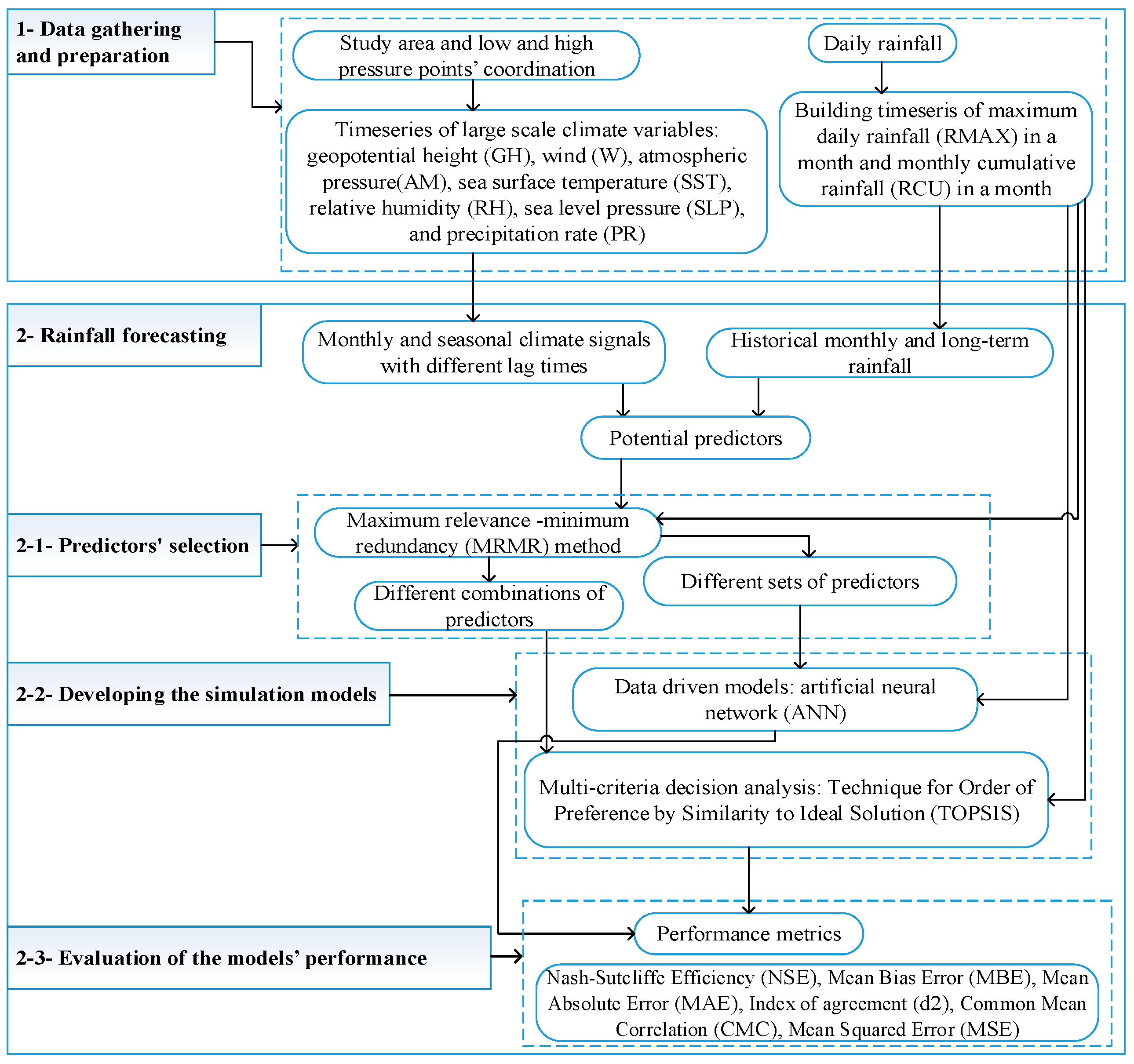
The flowchart presented in Figure 1 shows the proposed scheme of this study to forecast rainfall.
3.1. Data Gathering and Preparation
Two sets of rainfall timeseries i.e., maximum daily rainfall (RMAX) in a month, and monthly cumulative rainfall (RCU) in a month, are considered as the forecasting targets. These rainfall timeseries are formed using the daily data obtained from the gauge station presented in Table 1. In order to constitute the rainfall models’ input set, monthly timeseries of large scale climate signals, including geopotential height eight (GH), wind speed (W), air temperature (AM), SST, relative humidity (RH), SLP, and precipitation rate (PR) are attained from the National Ocean and Atmospheric Administration (NOAA) website (monthly/seasonal mean time series from the NCEP Reanalysis Dataset from http://esrl.noaa.gov/psd/cgi-bin/data/timeseries/timeseries1.pl). Climate signals data are available from March 1948 to present.
There is a high correlation between the large scale climate signals over the North-Eastern Pacific and the extreme hydrologic events across the North America West Coast [15,41]. One example is the SLP over the North Pacific Ocean which is dominated by the “North Pacific High” (a well-developed high pressure system located in the northeastern part of the Pacific Ocean) [42]. This high pressure system has the strongest effects on the storms during the northern hemisphere summer and causes dry summers and falls, and wet winters and springs over the western parts of Unites States [43]. According to Bonsal et al. [44], there is a strong relation between large scale teleconnections (patterns of pressure and circulation anomalies that span long distant geographical areas) and Canadian climate. In this study, to investigate the relationship between the large scale climate signals over the North Pacific Ocean and extreme rainfall for the study area, climate data are downloaded for four different regions (here called characteristic locations). One of these regions covers the study area (i.e., 110°–130° W longitude and 48.6°–54.4° N Latitude, shown by L1), and the rest of them (indicated by L2, L3, and L4) cover low and high pressure points on the North Eastern Pacific Ocean, with coordinates 120°–150° W and 50°–70° N, 140°–180° W and 40°–60° N, and 100°–120° W and 40°–50° N, respectively. Figure 2 shows the locations of the selected regions for acquiring large scale climate signals.
The list of climate variables for location L1 is shown in Table 3 (rows 1 to 9). SST and SLP monthly anomalies (rows 6 and 8 in Table 3) are calculated by subtracting long-term average of SST and SLP over each month from the observed SST and SLP for the corresponding month. Likewise, SST and SLP seasonal anomalies (rows 7 and 9 in Table 3) are calculated by subtracting seasonal SST and SLP for all seasons from the monthly values of observed SST and SLP corresponding to each season.
Four lag times (1 month, and 2, 3 and 12 months) are considered. Based on these lag times, a total of 47 predictors for location L1 are constructed (shown by L11 to L147 in Table 3). Therefore, for four locations, a total of 188 (47 × 4) timeseries of climate signals are developed. In addition to the large scale climate signals with various lag times, historical rainfalls (historical RMAX and RCU) are also incorporated in constructing the predictors’ sets (the last four rows in Table 3). This means that for example, to forecast rainfall for April 2016, rainfall values for March, February and January 2016, as well as April 2015, may be used (i.e., RMAX1–RMAX4 and RCU1–RCU4). RMAXL and RCUL in Table 3 signify the long term average of monthly rainfalls for 12 months (i.e., January to December). Therefore, for RMAX and RCU, by averaging the data for the entire time period, 12 values are obtained, and then for each month, the corresponding long term average of rainfall is used in the predictors’ set. Adding the timeseries built from the historical rainfall to the large scale climate signals, 198 (188 + 10) predictors will be considered for rainfall forecasting.
3.2. Rainfall Forecasting
Two rainfall values are considered to be forecasted: monthly maximum daily rainfall (RMAX) (the maximum value of daily rainfall in a month) and monthly cumulative value of rainfall (RCU) (cumulative values of daily rainfalls for a month).
One of the main issues in developing predictive tools is to select the most appropriate set of predictors. Taking into account four locations (L1–L4), and monthly and seasonal climate signals with different lag times (1, 2, 3 and 12 months), a large set of possible combinations of predictors can be built. Different feature selection methods, such as Mutual Information [45], stepwise regression [46] and Max-Relevance and Min-Redundancy [45,47] can be used for selecting the optimal input variables. Considering the findings of the previous studies and the efficiency of these methods, in this study Max-Relevance and Min-Redundancy (MRMR) method is employed to select the most appropriate predictors’ set with efficient number of climate signals. MRMR considers the correlation between input variables (predictors) and rainfall (predictant), as well as inter-correlation between the inputs. The forecasting models use the identified variables by MRMR as input (predictors) and, RMAX and RCU as target (predictant).
3.2.1. Predictors’ Selection for Rainfall Forecasting: Application of MRMR Method
For data driven models, inputs have substantial effect on the model simulation performance. Mutual information (MI)-based methods are tools used to select the most suitable inputs. MRMR is an example of these methods. It selects a set of predictors among a large number of predictors (features) that are related to a predictant. This method can pick out a set of appropriate inputs based on the desired number of predictor variables. The selected predictors have the highest MI with predictant (target) and the lowest MI among themselves.
MI for two random variables of and is shown by . is defined based on their probabilistic density functions represented by , , and , respectively:
The purpose of MI is to find a set of predictors (called A) with k features that jointly have the largest dependency on the target class :
MRMR is represented by the criteria of maximum relevance (Max-R) and minimum redundancy (Min-R). In Max-R, selected features () among the predictors are required to individually have the largest MI with predictant (c). This reflects a large dependency with the target. Max-R means to find predictors satisfying Equation (3). This equation approximates with the mean value of all MI’s between (the ith feature) and :
In the feature selection, selecting combinations of individually good features do not necessarily lead to a good performance for the classification. This is due to the redundancy among features. Therefore, the following Min-R condition is added to select mutually exclusive features with minimum redundancy:
MRMR merges the above two max and min constraints. Then, the Φ operator combines and to maximize and minimize simultaneously:
Here, the maximum number of features (k) in the predictors’ set is considered to be 50 (i.e., 4 ≤ k ≤ 50). In the MRMR method, predictors are selected based on their order of correlation with the predictant. In other words, by increasing the value of k, a new predictor is added to the previous set of inputs.
3.2.2. Models’ Development
Two modeling approaches are employed for rainfall simulation and forecasting. The first approach is based on the application of artificial neural network (ANN) machine learning method. The second model uses a multi-criteria decision analysis method, called Technique for Order of Preference by Similarity to Ideal Solution (TOPSIS).
● Data driven models for rainfall forecasting: application of artificial neural network (ANN)
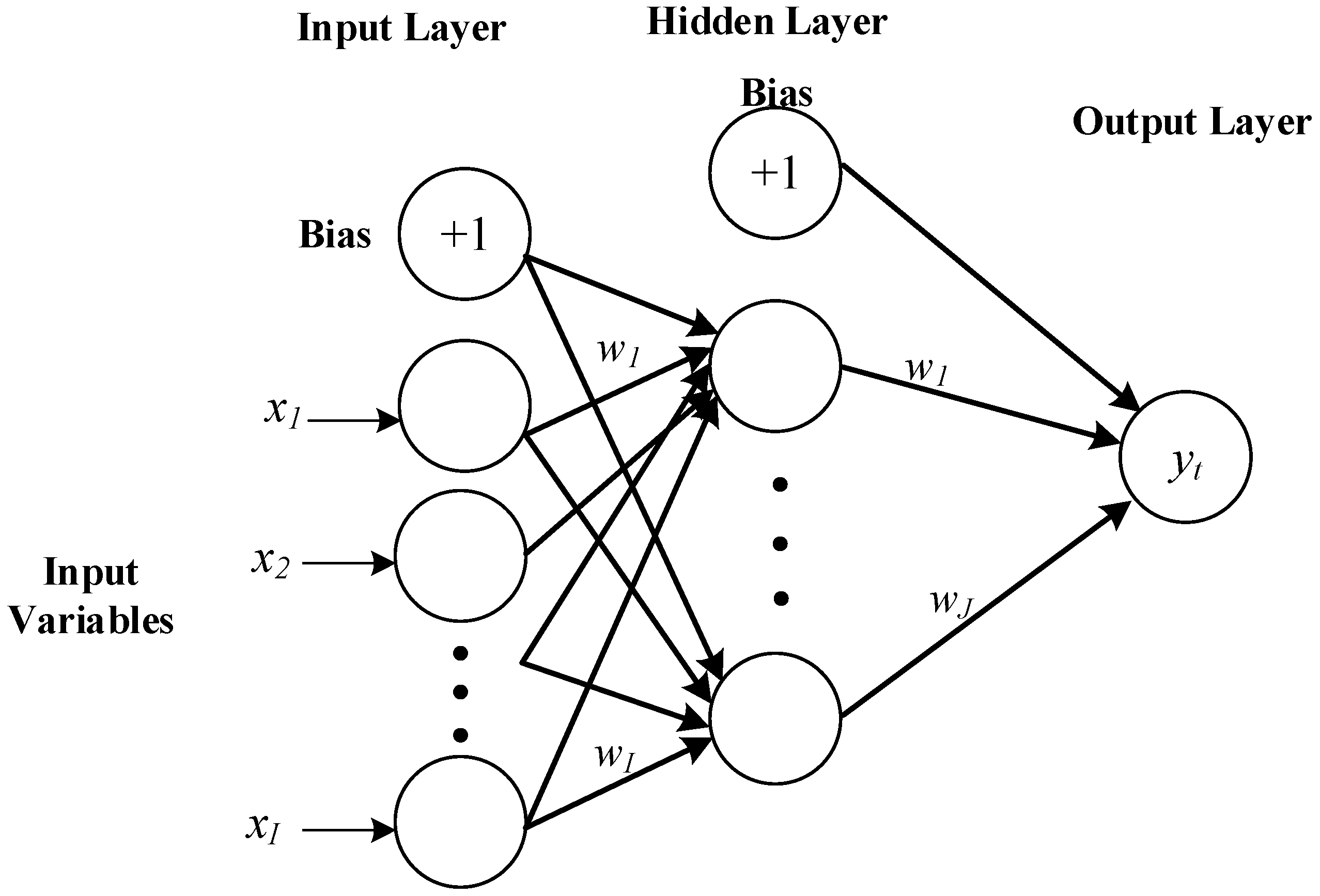
ANNs are composed of a system of interconnected neurons that fed by predictors (inputs) and compute outputs by feeding information through layers of neurons in the network (Figure 3).
In this study, Multi-Layer Perceptron (MLP) neural network models (feedforward networks that consists of the input layer, the hidden layers and the output layer, and process the information from the input layer to the hidden layer and then the output layer) with various structures are tested:
where is the output, is the input, and and are the weights between neurons of the input and hidden layer and between the hidden layer and output, respectively. and are the bias vectors for the input and hidden layers, and and are the activation functions for the output layer and the hidden layer, respectively. Also, I and J signify the number of nodes in the input and hidden layer [28].
Networks with 1 hidden layer with the number of neurons allowed to vary between 2 and 40 are built [48]. To test if the network simulation performance could be improved, models are checked with logsig (Log-sigmoid) and tansig (Hyperbolic tangent sigmoid) non-linear transfer functions for the hidden layer ( in Equation (7)). Moreover, different training functions including traingdm (Gradient descent with momentum backpropagation), trainlm (Levenberg-Marquardt backpropagation) and traingdx (Gradient descent with momentum and adaptive learning rate backpropagation) are also examined. For the MLP networks, output unit is selected to be the linear purelin (pure linear) function ( In Equation (8)). The number of inputs in each time step is equal to the number of the selected predictors by MRMR. The initial weights are randomly selected, and then to obtain the best simulation, weights are adjusted during the network training. More information about the application of artificial neural networks can be found in [49]. A vector composed of historical observed rainfall is used for supervised network training using the back propagation algorithms. 70% of data is used for calibration, 20% for validation, and 10% for forecasting.
Set of the input data for the networks is built by choosing predictors from the first 50 variables selected among the 198 predictors by MRMR. The minimum number of predictors in the input set is 4 and the maximum number of predictors is 50. To automate the process of constructing the models (with different structures and number of input predictors) and find the model with the highest simulation performance, the whole process is scripted in MATLAB. Several metrics (Equations (17)–(22)) are used to evaluate the goodness of fit of the models’ performance, and finally choose the ANN model with an optimized structure.
● Multi-criteria decision analysis method for rainfall forecasting: Technique for Order of Preference by Similarity to Ideal Solution (TOPSIS)
TOPSIS is a multi-criteria decision analysis ranking technique. The efficiency of TOPSIS method to forecast rainfall is investigated in this study. In this technique, the chosen alternative (here is the rainfall event) should have the shortest and longest distances from the positive ideal and negative ideal solutions (selected among the historical rainfall events), respectively. With m alternatives (number of the events in the time series of historical rainfall) and n criteria (number of the selected predictors), a decision matrix () should be built. Given the large number of identified variables (i.e., 198), MRMR method is employed for the selection of the variables to form the predictors’ set (MRMR is set up to select the first 50 most relevant variables). It is decided to test different sets of criteria by letting n changes between 1 and 50. Then, all possible combinations of variables based on the selection of n criteria among 50 variables are checked (i.e., where 1 ≤ n ≤ 50). Consequently, with different values of n, a large number of decision matrices could be developed. Developed modeling approach based on TOPSIS is applied for both timeseries of rainfall, i.e., RMAX and RCU.
Based on n criteria and m alternatives, the decision matrix can be transformed to a non-dimensional normalized decision matrix ():
Thereafter, the weighted normalized decision matrix () is built:
where , which is the weight given to each predictor (criteria), is considered to be 1. Then, the worst and the best alternatives (negative ideal and positive ideal solutions), and respectively, are determined:
where and are associated with the criteria having a positive and negative impact, respectively. In the following, distances between alternative and and , (shown by and , respectively) are calculated:
Finally, the relative closeness to and is determined:
is equal to 0 or 1, if and only if the identified solution has the worst or the best conditions, respectively.
Among the observed events in the rainfall timeseries (i.e., m alternatives), the last 10% of the events are kept to check the performance of the forecasting models. The rest of observed data are used to build the models. In other words, for each of the last 10% of the events, the model will look into the rest of the events (i.e., m − 10% × m events) to find the worst and the best alternatives and then identify the alternative with the highest value of relative closeness based on Equation (15).
To improve the performance of the TOPSIS models for the rainfall forecasting, instead of identifying only one alternative as the solution, 10 rainfall events with the highest values of relative closeness are selected. For this purpose, a set of alternatives is ranked according to the descending order of . Then, the ten alternatives with the highest values of are selected and combined using their corresponding relative weights:
where is the forecasted value of rainfall with one month lead time by TOPSIS, are the rainfall events with the highest values of relative closeness, and are the values of relative closeness corresponding to the identified rainfalls. This procedure is repeated for all of the rainfall events kept for checking the models’ performance, while models have different decision matrices. To identify the model with the ideal number of criteria (n), the models’ performance for rainfall forecasting should be compared.
3.3. Evaluation of the Forecasting Models’ Performance
The following metrics are used to analyze and compare the power of the developed models for rainfall simulation and forecasting:
where Oi and Si are observed and forecasted monthly rainfall in month i, respectively. and are the long term mean values of observed and forecasted monthly rainfall for the entire time period, respectively. NSE represents a measure of the proportion of the initial variance accounted for the model, and ranges between to +1 for a perfect correlation. MBE is a measurement of accuracy. MBE shows the difference between the expected value of rainfalls (forecast) and its true value (observation). MBE could be negative or positive, while values closer to zero are more preferable. MAE measures residual errors and provides information about the difference between the observed and forecasted values, while smaller values are more preferable. d2 compares the difference between the simulated and observed rainfall means and represents the degree of error in simulations [50,51,52]. d2 varies between 0, for complete disagreement, and 1 for perfect agreement between the observed and predicted data. CMC provides an informative measure of prediction performance and varies between 0 for weak and 1 for perfect performance [53]. MSE, the second moment of the bias (where bias is defined as an average of all errors), measures the average squares of the errors or deviations, which is the difference between the observed and forecasted rainfall. The MSE is a non-negative measure and values closer to zero are preferable.
4. Results and Discussion
In this section, results, for selecting the set of predictors, models’ development for rainfall simulation and then comparing the models’ performances, are presented according to the order of the methodology steps introduced in Figure 2.
4.1. MRMR Method: Selecting the Most Effective Predictors for Rainfall Forecasting
Table 4 and Table 5 list the selected 50 predictors identified using the MRMR method to forecast RMAX and RCU. In these Tables, rank represents the preference order of the variable relative to the rainfall forecast, i.e., the lower ranks are associated with more appropriate predictors.
Table 4 and Table 5 confirm that among the large scale climate signals, geopotential height (GH) is repeated more than the other signals (for all characteristic locations L1 to L4). Then, SST and SLP signals and anomalies are reported more frequently. Moreover, these tables suggest that historical values of rainfall (i.e., RMAX and RCU with different lag times) could be of significant effect for rainfall forecasting. For RMAX variables, the most repeated lag times are 1 and 12, while for RCU variables, lag times of 3 and 12 months are repeated more than the others. Among the characteristic locations, for both RMAX and RCU, L4 is repeated more frequent than the other locations (14 times for RMAX and 19 times for RCU).
4.2. Rainfall Forecasting and Comparison of the Models’ Performance
4.2.1. Application of ANNs
Using the automated script in MATLAB, different possible structures of ANN models (various transfer functions, training algorithms and input variables) are tested and their performances to simulate the rainfall timeseries are reported and compared. Number of inputs to the networks is allowed to vary between 4 and 50. In other words, initially, the first 4 variables, listed in Table 4 (for RMAX) and Table 5 (for RCU), are used for simulation, and then the number of variables is increased until all the variables shown in these tables are used as inputs to the ANN models. Comparing the simulation results based on the performance metrics indicate that the models with “logsig” transfer function and “traingdx” back propagating algorithm perform better than other structures for simulation of RMAX. However, for the simulation of RCU, ANN models with “tansig” transfer function and “traingdx” back propagation algorithm revealed better simulation performance.
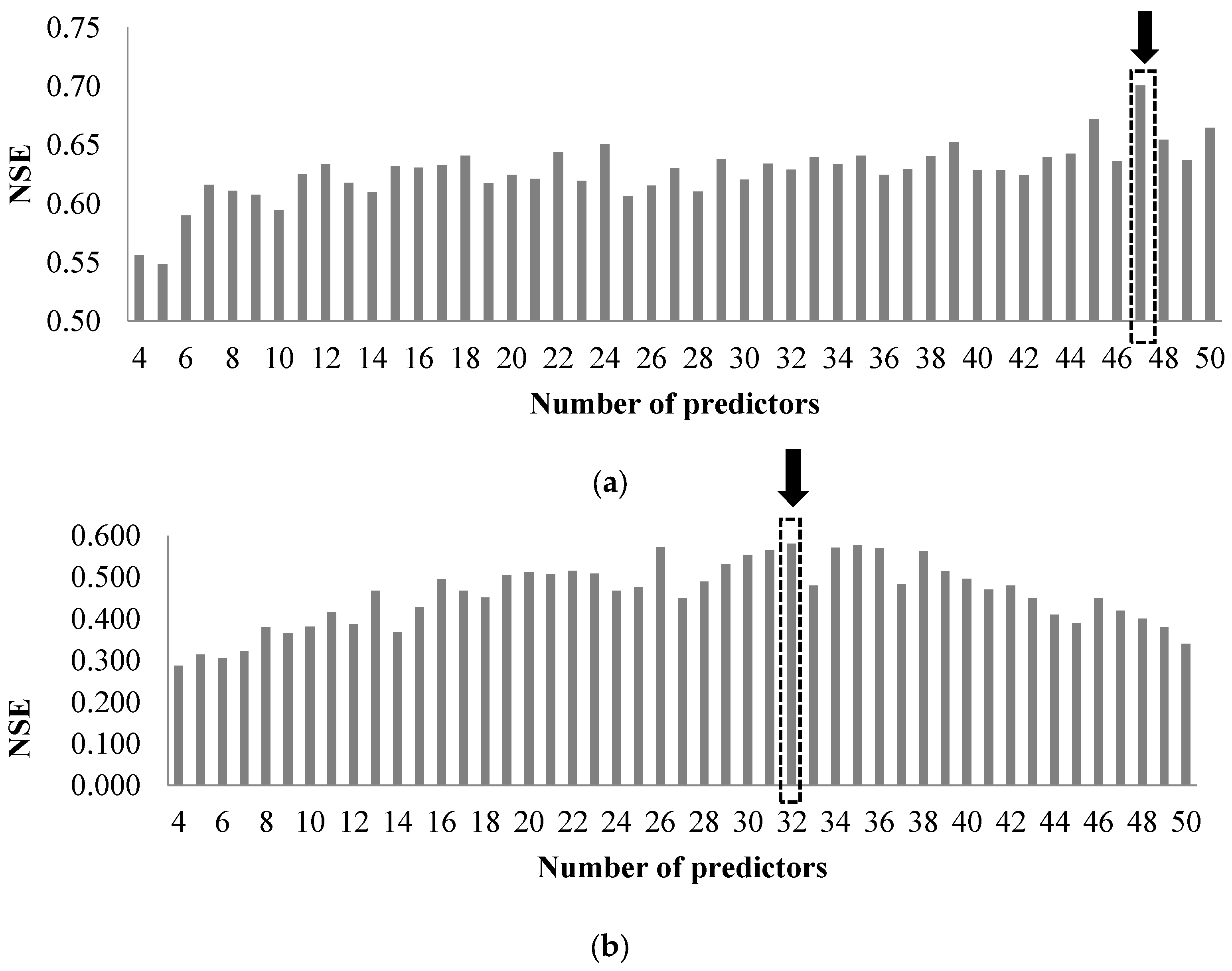
Figure 4 illustrates the NSE values for different ANNs with varying input variables and the above mentioned structures to simulate the RCU and RMAX. This figure is intended to depict how changes in the number of predictors could affect the modeling performance. The NSE metric shows the overall simulation performance of the model in the calibration and validation periods. Based on Figure 4a for RCU, the model with the first 47 predictors listed in Table 5 has the maximum value of NSE. Similarly, as shown in Figure 4b, the best ANN model uses the first 32 predictors listed in Table 4 for the simulation of RMAX. Number of neurons in the hidden layer for both models is 10.
Table 6 indicates the simulation performance of selected ANN models for the simulation of RCU and RMAX.
As Table 6 shows, although the simulation performance of the models in the calibration period is noticeably high, during the validation period the models do not perform well, particularly considering the NSE metric. Moreover, the number of selected predictors is relatively high (47 for RCU and 32 for RMAX). As mentioned in the methodology section, 10% of data are used for testing the models’ performance for forecasting rainfall. The structure of the models with the highest simulation performance in the calibration and validation period is saved. These models are then used with the testing data, as input, for forecasting rainfall. The results indicate that the performance of ANN models for the test period is not acceptable since they forecast negative values for rainfall. The models’ functionality in the validation and during the test periods confirms that machine learning ANN models fail in forecasting rainfall.
4.2.2. Application of TOPSIS
Data from April 1949 to December 2015 are used to build the decision matrix. From these data, the last 10% of the rainfall events are not used in the building of the matrix. Data in this period are considered as the forecasting targets (TOPSIS will look for the closest alternatives to these events among the other historical rainfalls, based on comparing the distance between the corresponding sets of predictors).
All possible combinations of input criteria (i.e., where 1 ≤ n ≤ 50), as predictors, are investigated to build the decision matrices for forecasting RCU and RMAX. Criteria are selected among those 50 predictors selected by MRMR shown in Table 4 and Table 5. For each value of n, the evaluation metrics are estimated for each individual combination and the best combination with the highest evaluation metric is picked.
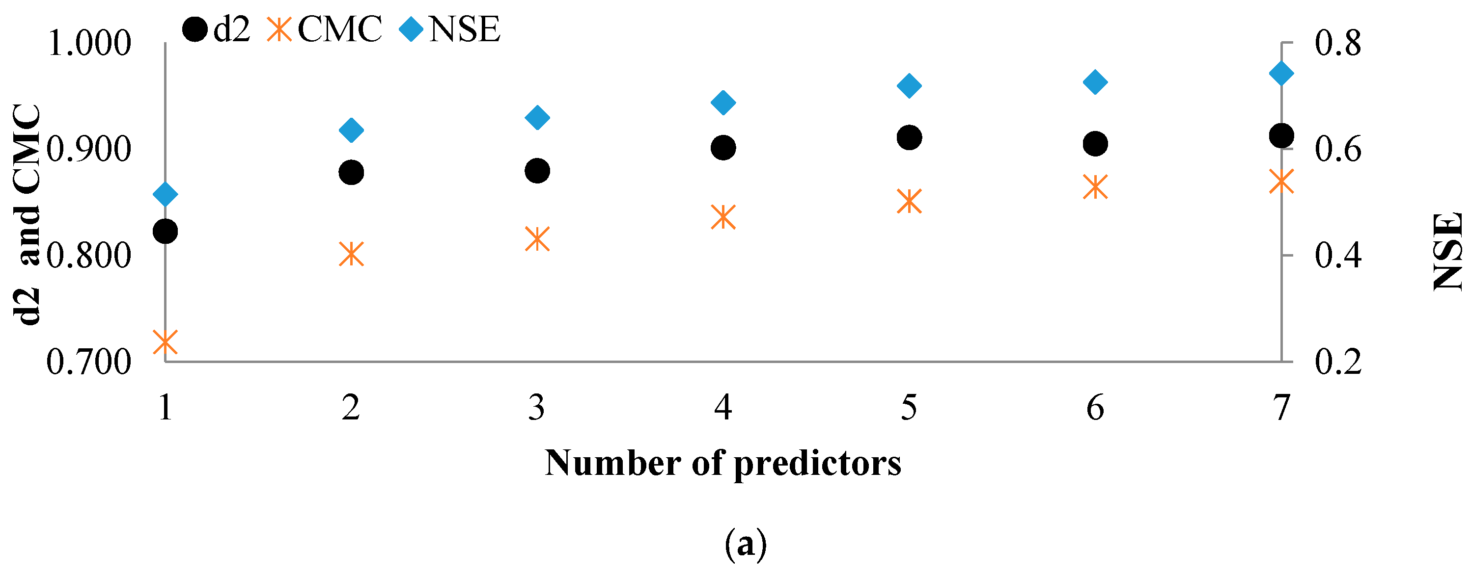
Results show that increasing n improves the modeling performance. Variations of d2, CMC and NSE performance metrics against the number of predictors for RCU and RMAX are shown in Figure 5. It can be seen that for n > 5, increases in the values of metrics are not significant. Moreover, running the models to check the performance of different combinations takes a considerable time (e.g., simulation run time can take up to a month for 15,890,700 combinations of variables when n = 6 →). Therefore, given the negligible increase in the simulation performance after n = 5, the maximum value of n is deemed to be 7.
Seven variables that are shown to result in the best performance of the TOPSIS model for forecasting RCU are shown in Table 7. Same wise, Table 8 indicates the six variables that resulted in the highest simulation performance of TOPSIS for RMAX.
Table 7 and Table 8 show how effective are GH and SST climate signals (with different lag times and at different characteristic locations) on rainfall forecasting. As for RCU, historical rainfall (cumulative precipitation with 3 months lag time and maximum precipitation with 2 months lag time) are also among the selected set of predictors. GH, SST and historical rainfall were also observed among the most repeated variables for rainfall simulation with the ANN models.
Figure 6 compares the observed monthly rainfalls (from November 2011 to November 2015) with those forecasted by TOPSIS (i.e., selected alternatives among the historical rainfall events from April 1949 to October 2011) for RCU and RMAX. To find these alternatives, TOPSIS finds the best and worst ideal solutions among the sets of predictors (i.e., timeseries of 7 criteria for RCU shown in Table 7, and timeseries of 6 criteria for RMAX shown in Table 8). These solutions have, respectively, the minimum and maximum distance from the values of the same criteria corresponding to each rainfall event subjected for forecasting. Forecasting rainfall by TOPSIS is based on comparing the current teleconnection conditions (the values of climate signals) with those already occurred in the past, then finding the most similar conditions and expecting the corresponding value of past rainfall to occur for the considered current conditions. This method works well when, on average, similar weather conditions happen through time. As shown in Figure 6, for both RCU and RMAX, some of the peak observed values are not caught by TOPSIS. This means that the recorded historical events do not incorporate weather conditions similar to those correspond to the extreme observed events.
Table 9 further illustrates the numerical performance of TOPSIS model for rainfall forecasting based on several evaluation metrics. Comparing the results with those obtained from ANN model shows that both modeling approaches outperform the simulation of monthly cumulative rainfall against maximum daily rainfall in a month.
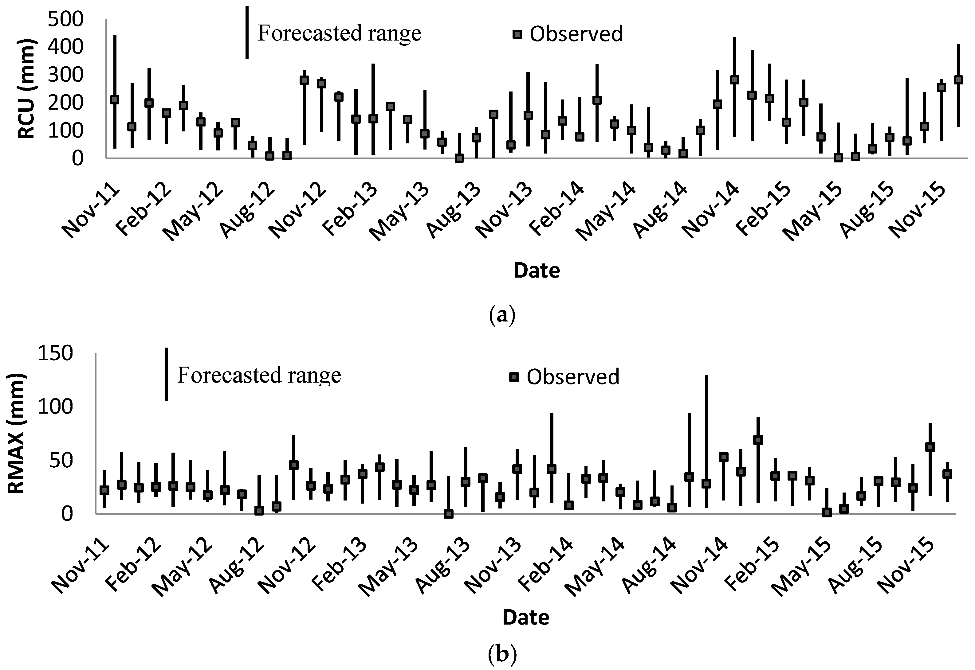
Since, as explained in the methodology and shown by Equation (13), for each observed rainfall event, TOPSIS identifies the 10 of the closest alternatives, it is possible to determine a range of variation (a confidence interval) for future rainfall looking into these 10 alternatives. To determine the lower and upper values for this range, the minimum and maximum values of rainfall among the 10 alternatives are identified and used. Figure 7 shows the obtained range of variation as the forecasted window for values of RCU and RMAX, from November 2011 to November 2015. Then, it is investigated if the observed value of rainfall, at each time step, falls within the identified forecasted window.
Results show that 48 out of 50 events for RCU and 46 out of 50 events for RMAX fall in the identified range at each time. Therefore, the developed TOPSIS model, not only performs relatively well in forecasting the individual values of rainfall, but also is capable of estimating a forecasting window for future RCU and RMAX with the accuracy of 96% and 92%, respectively.
5. Summary and Conclusions
In this study, a framework is suggested for forecasting rainfall for Vancouver area, BC, Canada. The monthly and seasonal large scale climate signals, at the identified low and high pressure characteristic locations in the North Pacific Ocean, and the extreme and cumulative monthly rainfall for the study area are investigated to develop long lead rainfall forecasting models. A feature selection method (MRMR) is used to select the most effective predictors among the set of climate variables identified for forecasting rainfall for western Canadian regions. Then, two approaches are examined for rainfall forecasting. The first approach is based on MLP data driven models (i.e., ANNs) and the second one is designed using a multi-criteria decision analysis method (i.e., TOPSIS). ANNs are known as powerful tools when used for the aim of modeling and simulation. However, based on the results, they fail for forecasting purposes. Although ANNs’ performance in the calibration period is promising, they do not show acceptable performance in the validation and then testing period (which corresponds to the data that are not used for the networks training in the calibration and validation periods). Moreover, a large number of predictors (47 for RCU and 32 for RMAX) have to be used to obtain a high simulation performance for ANNs. In contrast, the developed TOPSIS model, TOPSIS, performed well for rainfall forecasting with a few number of predictors (6 for RCU and 7 for RMAX). The TOPSIS model also shows high capability in forecasting the domain of rainfall occurrence (future confidence interval).
Occurrence of flooding is an un-stoppable reality, and reliable flood forecasting is a serious challenge that most of the Canadian provinces are dealing with. Heavy rainfall events are one of the main reasons for river overbanking, extreme freshets and surface runoff flooding in urban areas. Given the great uncertainty associated with hydro-meteorological predictions, the development of models for real time (e.g., one month lead time in this study) extreme rainfall forecasting provides an insight to the evaluation of possible weather conditions in a region. These forecasts, with an acceptable accuracy, are beneficial in short-term operation and management of water resources. This paper, as a pioneer study in forecasting long lead rainfall for western Canadian watersheds, shows how large scale climate signals can be effectively used to provide a reliable estimate for future rainfall. Forecasted maximum rainfall provides valuable information for the prediction of surface runoff and potential inland flood. The predicted range of variation for rainfall can also offer input for hydrologic modeling when uncertainties are considered to be incorporated in the analysis.
A small catchment has been selected in this study to develop the methodology. However, to expand this study, larger areas with multiple rainfall gauge stations can be selected to investigate the application of more rainfall data as input as well as if the proposed method could successfully forecast the range and value of an average value for rainfall for the whole study area. The data driven model which is used in this study, i.e., FFNN, showed low simulation performance in the validation period and not acceptable performance in the forecasting time. Other structures of artificial networks are suggested to be developed and checked for rainfall forecasting. Considering thousands of different combinations of predictors that result in a long run time for the TOPSIS model, desktop computers with higher speed configuration could be used to afford the computational efforts and investigate all possible combinations. Moreover, in constructing the decision matrix in the TOPSIS method, assigning unequal weights to the predictors could be analyzed. In addition to investigating the forecast of maximum daily rainfall, application of monthly large scale climate signals for forecasting average monthly rainfall could also be analyzed.
Author Contributions
Zahra Zahmatkesh designed the multi-criteria decision analysis model for rainfall forecasting. Erfan Goharian developed the neural networks. Zahra Zahmatkesh and Erfan Goharian analyzed the results. Zahra Zahmatkesh wrote the paper and Erfan Goharian reviewed and provided feedback on paper.
Conflicts of Interest
The authors declare no conflict of interest.
References
- Rodda, J.C.; Rodda, H.J.E. Hydrological forecasting. In Dealing with Natural Disasters: Achievements and New Challenges in Science; The Royal Society: London, UK, 1999; pp. 75–99. [Google Scholar]
- Balica, S.F.; Popescu, I.; Beevers, L.; Wright, N.G. Parametric and physically based modelling techniques for flood risk and vulnerability assessment: A comparison. Environ. Model. Softw. 2013, 41, 84–92. [Google Scholar] [CrossRef]
- Jonkman, S.N. Global perspectives on loss of human life caused by floods. Nat. Hazards 2005, 34, 151–175. [Google Scholar] [CrossRef]
- Thiele-Eich, I.; Burkart, K.; Simmer, C. Trends in water level and flooding in Dhaka, Bangladesh and their impact on mortality. Int. J. Environ. Res. Public Health 2015, 12, 1196–1215. [Google Scholar] [CrossRef] [PubMed]
- Goharian, E.; Burian, S.J.; Lillywhite, J.; Hile, R. Vulnerability assessment to support integrated water resources management of metropolitan water supply systems. J. Water Resour. Plan. Manag. 2016, 143, 04016080. [Google Scholar] [CrossRef]
- Goharian, E.; Burian, S.J.; Bardsley, T.; Strong, C. Incorporating potential severity into vulnerability assessment of water supply systems under climate change conditions. J. Water Resour. Plan. Manag. 2015, 142, 04015051. [Google Scholar] [CrossRef]
- Zahmatkesh, Z.; Karamouz, M.; Goharian, E.; Burian, S. Analysis of the Effects of Climate Change on Urban Storm Water Runoff Using Statistically Downscaled Precipitation Data and a Change Factor Approach. J. Hydrol. Eng. 2014. [Google Scholar] [CrossRef]
- Manitoba 2011 Flood Review Task Force (MFRTF). Report to the Minister of Infrastructure and Transportation 2013. Available online: https://www.gov.mb.ca/asset_library/en/2011flood/flood_review_task_force_report.pdf (accessed on 25 June 2017).
- Pomeroy, J.W.; Stewart, R.E.; Whitfield, P.H. The 2013 flood event in the South Saskatchewan and Elk River basins: Causes, assessment and damages. Can. Water Resour. J. 2016, 41, 105–117. [Google Scholar] [CrossRef]
- Rasmussen, P.F. Evaluation of Flood Forecasting and Warning Systems in Canada. In Proceedings of the CSCE 22nd Canadian Hydrotechnical Conference 2015, Montreal, QC, Canada, 29 April–2 May 2015. [Google Scholar]
- Zahmatkesh, Z.; Burian, S.J.; Karamouz, M.; Tavakol-Davani, H.; Goharian, E. Low-impact development practices to mitigate climate change effects on urban stormwater runoff: Case study of New York City. J. Irrig. Drain. Eng. 2014, 141, 04014043. [Google Scholar] [CrossRef]
- Taksande, A.A.; Khandait, S.P.; Katkar, M. Rainfall Forecasting Using Artificial Neural Network: A Data Mining Approach. Int. J. Eng. Sci. Res. Technol. 2014, 1, 2018–2020. [Google Scholar]
- Goharian, E. A Framework for Water Supply System Performance Assessment to Support Integrated Water Resources Management and Decision Making Process. Ph.D. Thesis, University of Utah, Salt Lake City, UT, USA, August 2016. [Google Scholar]
- Hansen, C.H.; Goharian, E.; Burian, S. Downscaling Precipitation for Local-Scale Hydrologic Modeling Applications: Comparison of Traditional and Combined Change Factor Methodologies. J. Hydrol. Eng. 2017, 22, 04017030. [Google Scholar] [CrossRef]
- Favre, A.; Gershunov, A. Extra-tropical cyclonic/anticyclonic activity in North-Eastern Pacific and air temperature extremes in Western North America. Clim. Dyn. 2006, 26, 617–629. [Google Scholar] [CrossRef]
- Zahmatkesh, Z.; Karamouz, M.; Nazif, S. Uncertainty based modeling of rainfall-runoff: Combined differential evolution adaptive metropolis (DREAM) and K-means clustering. Adv. Water Resour. 2015, 83, 405–420. [Google Scholar] [CrossRef]
- Nicholson, S.E.; Selato, J.C. The Influence of La Nina on African Rainfall. Int. J. Climatol. 2000, 20, 1761–1776. [Google Scholar] [CrossRef]
- Mariotti, A.; Zeng, N.; Lau, K.M. Euro-Mediterranean rainfall and ENSO—A seasonally varying relationship. Geophys. Res. Lett. 2002, 29, 59–61. [Google Scholar] [CrossRef]
- Verdon, D.C.; Franks, S.W. Indian Ocean sea surface temperature variability and winter rainfall: Eastern Australia. Water Resour. Res. 2005, 41, 477–487. [Google Scholar] [CrossRef]
- Ashok, K.; Behera, S.K.; Rao, S.A.; Weng, H.; Yamagata, T. El Niño Modoki and its possible teleconnection. J. Geophys. Res. Oceans 2007, 112. [Google Scholar] [CrossRef]
- Preethi, B.; Sabin, T.P.; Adedoyin, J.A.; Ashok, K. Impacts of the ENSO Modoki and other tropical Indo-Pacific climate-drivers on African rainfall. Sci. Rep. 2015, 5. [Google Scholar] [CrossRef] [PubMed]
- Choubin, B.; Malekian, A.; Golshan, M. Application of several data-driven techniques to predict a standardized precipitation index. Atmósfera 2016, 29, 121–128. [Google Scholar] [CrossRef]
- Wang, Q.J.; Schepen, A.; Robertson, D.E. Merging seasonal rainfall forecasts from multiple statistical models through Bayesian model averaging. J. Clim. 2012, 25, 5524–5537. [Google Scholar] [CrossRef]
- Ramirez, M.C.V.; de Campos Velho, H.F.; Ferreira, N.J. Artificial neural network technique for rainfall forecasting applied to the Sao Paulo region. J. Hydrol. 2005, 301, 146–162. [Google Scholar] [CrossRef]
- Huong, H.T.L.; Pathirana, A. Urbanization and climate change impacts on future urban flooding in Can Tho city, Vietnam. Hydrol. Earth Syst. Sci. 2013, 17, 379–394. [Google Scholar] [CrossRef]
- Janga Reddy, M.; Maity, R. Regional rainfall forecasting using large scale climate teleconnections and artificial intelligence techniques. J. Intell. Syst. 2007, 16, 307–322. [Google Scholar]
- Karamouz, M.; Fallahi, M.; Nazif, S.; Rahimi Farahani, M. Long Lead Rainfall Prediction Using Statistical Downscaling and Artifcial Neural Network Modeling. Trans. A Civ. Eng. 2009, 16, 165–172. [Google Scholar]
- Mekanik, F.; Imteaz, M.A.; Talei, A. Seasonal rainfall forecasting by adaptive network-based fuzzy inference system (ANFIS) using large scale climate signals. Clim. Dyn. 2016, 46, 3097–3111. [Google Scholar] [CrossRef]
- Luk, K.C.; Ball, J.E.; Sharma, A. A study of optimal model lag and spatial inputs to artificial neural network for rainfall forecasting. J. Hydrol. 2000, 227, 56–65. [Google Scholar] [CrossRef]
- Nasseri, M.; Asghari, K.; Abedini, M.J. Optimized scenario for rainfall forecasting using genetic algorithm coupled with artificial neural network. Expert Syst. Appl. 2008, 35, 1415–1421. [Google Scholar] [CrossRef]
- Hong, W.C. Rainfall forecasting by technological machine learning models. Appl. Math. Comput. 2008, 200, 41–57. [Google Scholar] [CrossRef]
- Goharian, E.; Zahmatkesh, Z.; Sandoval-Solis, S. Uncertainty Propagation of Hydrologic Modeling in Water Supply System Performance: Application of Monte Carlo Markov Chain Method. J. Hydrol. Eng. 2018. [Google Scholar] [CrossRef]
- Kabiri, S.; Kalbkhani, H.; Lotfollahzadeh, T.; Shayesteh, M.G.; Solouk, V. Technique for order of preference by similarity to ideal solution based predictive handoff for heterogeneous networks. IET Commun. 2016, 10, 1682–1690. [Google Scholar] [CrossRef]
- Ozturk, D.; Batuk, F. Technique for order preference by similarity to ideal solution (TOPSIS) for spatial decision problems. In Proceedings of the GeoInformation for Disaster Management (Gi4DM 2011), Antalya, Turkey, 3–8 May 2011. [Google Scholar]
- Roshan, G.; Mirkatouli, G.; Shakoor, A. A new approach to technique for order-preference by similarity to ideal solution (TOPSIS) method for determining and ranking drought: A case study of Shiraz station. Int. J. Phys. Sci. 2012, 7, 2994–3008. [Google Scholar]
- Sikder, S.; Hossain, F. Assessment of the weather research and forecasting model generalized parameterization schemes for advancement of precipitation forecasting in monsoon-driven river basins. J. Adv. Model. Earth Sys. 2016, 8, 1210–1228. [Google Scholar] [CrossRef]
- Oulahen, G.; Mortsch, L.; Tang, K.; Harford, D. Unequal vulnerability to flood hazards: “Ground truthing” a social vulnerability index of five municipalities in Metro Vancouver, Canada. Ann. Assoc. Am. Geogr. 2015, 105, 473–495. [Google Scholar] [CrossRef]
- Forseth, P. Adaptation to Sea Level Rise in Metro Vancouver: A Review of Literature for Historical Sea Level Flooding and Projected Sea Level Rise in Metro Vancouver; Adaptation to Climate Change Team (ACT), Simon Fraser University: Vancouver, BC, Canada, 2012. [Google Scholar]
- BC Ministry of Environment. Climate Change Adaptation Guidelines for Sea Dikes and Coastal Flood Hazard Land Use: Guidelines for Management of Coastal Flood Hazard Land Use; Ausenco Sandwell: Vancouver, BC, Canada, 2011.
- Hallegatte, S.; Green, C.; Nicholls, R.J.; Corfee-Morlot, J. Future flood losses in major coastal cities. Nat. Clim. Change 2013, 3, 802–806. [Google Scholar] [CrossRef]
- Lu, R.; Dong, D.W. Westward extension of North Pacific subtropical high in summer. J Meteorol. Soc. Jpn. 2001, 79, 1229–1241. [Google Scholar] [CrossRef]
- Paek, H.; Yu, J.Y.; Zheng, F.; Lu, M.M. Impacts of ENSO diversity on the western Pacific and North Pacific subtropical highs during boreal summer. Clim. Dyn. 2016, 1–20. [Google Scholar] [CrossRef]
- Polade, S.D.; Gershunov, A.; Cayan, D.R.; Dettinger, M.D.; Pierce, D.W. Precipitation in a warming world: Assessing projected hydro-climate changes in California and other Mediterranean climate regions. Sci. Rep. 2017, 7. [Google Scholar] [CrossRef] [PubMed]
- Bonsal, B.; Shabbar, A. Impacts of large-scale circulation variability on low streamflows over Canada: A review. Can. Water Resour. J. 2008, 33, 137–154. [Google Scholar] [CrossRef]
- Karamouz, M.; Zahmatkesh, Z.; Nazif, S.; Razmi, A. An evaluation of climate change impacts on extreme sea level variability: Coastal area of New York City. Water Resour. Manag. 2014, 28, 3697–3714. [Google Scholar] [CrossRef]
- Karamouz, M.; Nazif, S.; Zahmatkesh, Z. Self-organizing gaussian-based downscaling of climate data for simulation of urban drainage systems. J. Irrig. Drain. Eng. 2013, 139, 98–112. [Google Scholar] [CrossRef]
- Karamouz, M.; Zahmatkesh, Z.; Goharian, E.; Nazif, S. Combined Impact of Inland and Coastal Floods: Mapping Knowledge Base for Development of Planning Strategies. J. Water Resour. Plan. Manag. 2014, 141. [Google Scholar] [CrossRef]
- Linoff, G.; Berry, M.J. Data mining Techniques: For Marketing, Sales, and Customer Support, 3rd ed.; John Wiley & Sons, Inc.: Hoboken, NJ, USA, 2011; ISBN 978-0-471-47064-9. [Google Scholar]
- Hassoun, M.H. Fundamentals of Artificial Neural Networks; MIT press: Cambridge, MA, USA, 1995; ISBN 9780262082396. [Google Scholar]
- Gardner, M.W.; Dorling, S.R. Statistical surface ozone models: An improved methodology to account for non-linear behaviour. Atmos. Environ. 2000, 34, 21–34. [Google Scholar] [CrossRef]
- Chaloulakou, A.; Saisana, M.; Spyrellis, N. Comparative assessment of neural networks and regression models for forecasting summertime ozone in Athens. Sci. Total Environ. 2003, 313, 1–13. [Google Scholar] [CrossRef]
- Sousa, S.I.V.; Martins, F.G.; Alvim-Ferraz, M.C.M.; Pereira, M.C. Multiple linear regression and artificial neural networks based on principal components to predict ozone concentrations. Environ. Model. Softw. 2007, 22, 97–103. [Google Scholar] [CrossRef]
- Iliadis, L.; Spartalis, S.; Tachos, S. An innovative artificial neural network evaluation model: Application in industry. In Proceedings of the 10th EANN Conference, Thessaloniki, Greece, 29–31 August 2007; pp. 320–327. [Google Scholar]
Figure 1.
Proposed methodology flowchart for large scale rainfall forecasting.

Figure 2.
Location of the selected areas to obtain large scale climate signals for rainfall forecasting for Vancouver.
Figure 2.
Location of the selected areas to obtain large scale climate signals for rainfall forecasting for Vancouver.
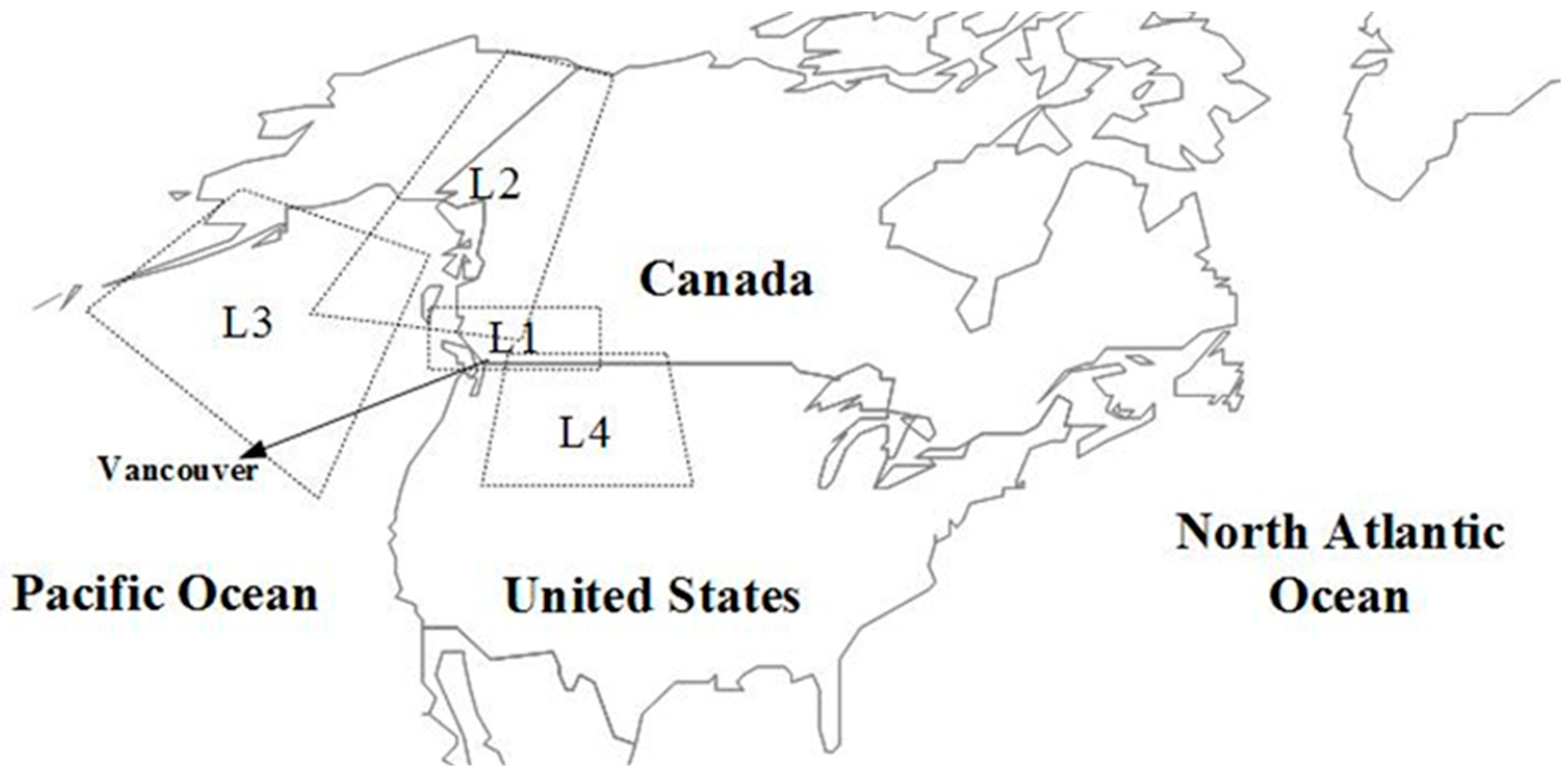
Figure 3.
Schematic of an artificial neural network model.

Figure 4.
Variation of evaluation metric CE against increasing the number of predictors for simulation of (a) RCU and (b) RMAX with ANN model.
Figure 4.
Variation of evaluation metric CE against increasing the number of predictors for simulation of (a) RCU and (b) RMAX with ANN model.

Figure 5.
Increasing the rainfall forecasting performance by increasing the number of variables in the predictors’ set for TOPSIS method, (a) RCU and (b) RMAX.
Figure 5.
Increasing the rainfall forecasting performance by increasing the number of variables in the predictors’ set for TOPSIS method, (a) RCU and (b) RMAX.

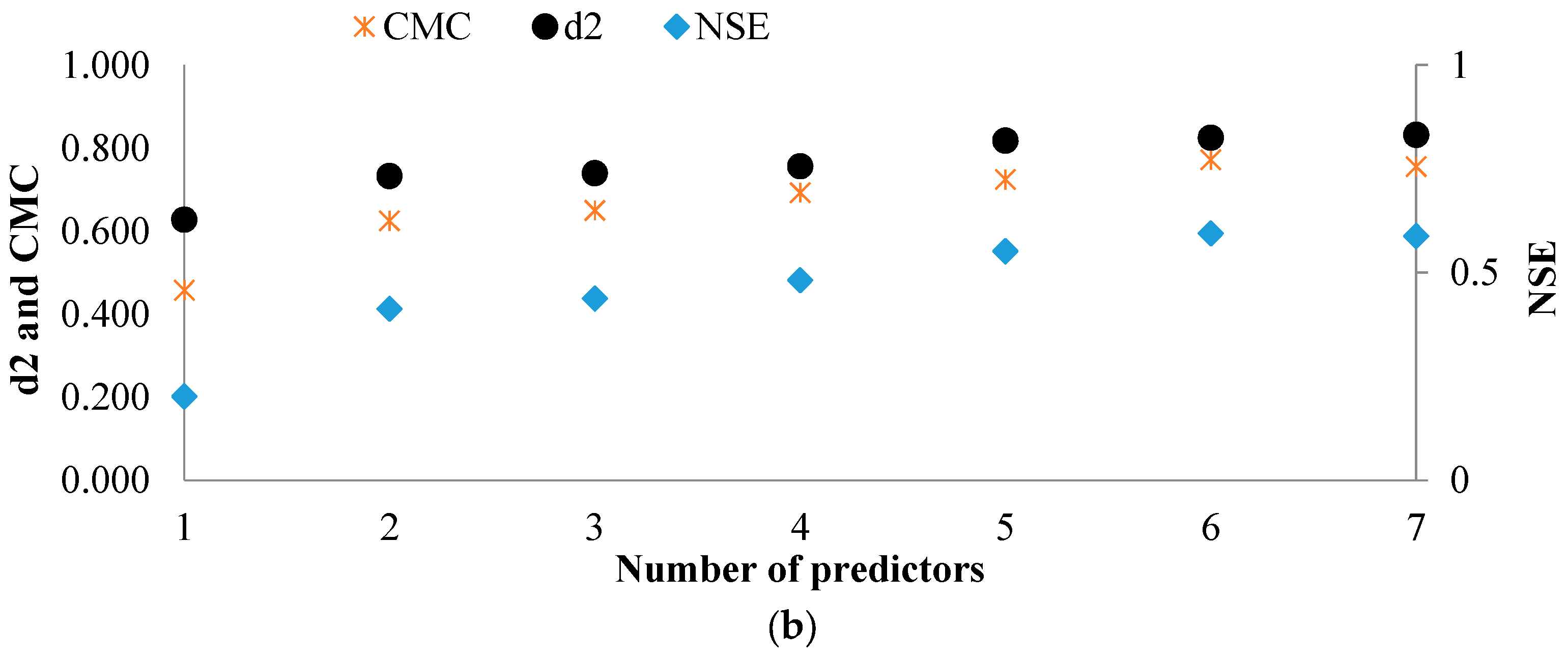
Figure 6.
Comparison of the observed rainfall with the forecasted values by TOPSIS for (a) RCU and (b) RMAX.
Figure 6.
Comparison of the observed rainfall with the forecasted values by TOPSIS for (a) RCU and (b) RMAX.
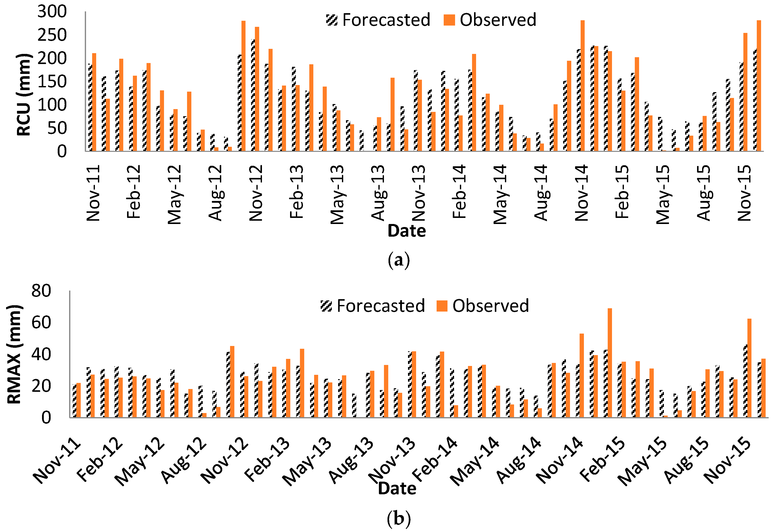
Figure 7.
Forecasted range of variation by TOPSIS for (a) RCU and (b) RMAX.

Table 1.
Characteristics of the rainfall gauge station in the study area.
| Name of the Station | Latitude (°) | Longitude (°) | Elevation (m) | Data Type and Length |
|---|---|---|---|---|
| Vancouver Harbour CS | 49.3 | −123.12 | 2.5 | daily precipitation (1925–present) |
Table 2.
Long term average for RMAX and RCU per mm based on the historical records of the observed data in Vancouver Harbour CS gauge station.
Table 2.
Long term average for RMAX and RCU per mm based on the historical records of the observed data in Vancouver Harbour CS gauge station.
| Month | Long Term Average | ||||||||||||
|---|---|---|---|---|---|---|---|---|---|---|---|---|---|
| Jan. | Feb. | Mar. | Apr. | May | Jun. | Jul. | Aug. | Sep. | Oct. | Nov. | Dec. | ||
| RMAX | 42.2 | 32.4 | 34.2 | 25.6 | 20.7 | 20.6 | 18.3 | 18.3 | 24.0 | 37.6 | 44.0 | 44.0 | 30.2 |
| RCU | 211.9 | 149.2 | 156.1 | 107.2 | 75.6 | 65.6 | 43.6 | 49.9 | 74.2 | 157.8 | 228.4 | 228.4 | 129.0 |
Table 3.
List of the large scale climate and precipitation variables considered to develop the rainfall forecasting model.
Table 3.
List of the large scale climate and precipitation variables considered to develop the rainfall forecasting model.
| ID | Variable |
|---|---|
| L11–L17 | GH, W, AM, SST, RH, SLP, and PR with 1 month lag time |
| L18–L114 | GH, W, AM, SST, RH, SLP, and PR with 2 months lag time |
| L115–L121 | GH, W, AM, SST, RH, SLP, and PR with 3 months lag time |
| L122–L128 | GH, W, AM, SST, RH, SLP, and PR average for the previous 3 months |
| L129–L131 | SST monthly anomalies with 1 month, and 2 and 3 months lag time |
| L132–L134 | SST seasonal anomalies with 1 month, and 2 and 3 months lag time |
| L135–L137 | SLP monthly anomalies with 1 month, and 2 and 3 months lag time |
| L138–L140 | SLP seasonal anomalies with 1 month, and 2 and 3 months lag time |
| L141–L147 | GH, W, AM, SST, RH, SLP, and PR with 12 months lag time |
| L21–L247 | Identified variables for location L2 (as similarly named by L11 to L147 for location L1) |
| L31–L347 | Identified variables for location L3 (as similarly named by L11 to L147 for location L1) |
| L41–L447 | Identified variables for location L4 (as similarly named by L11 to L147 for location L1) |
| RMAX1–RMAX4 | RMAX with 1 month, and 2, 3 and 12 months lag time |
| RCU1–RCU4 | RCU with 1 month, and 2, 3 and 12 months lag time |
| RMAXL | Long term monthly averages of RMAX (from January to December) |
| RCUL | Long term monthly averages of RCU (from January to December) |
Table 4.
Rank and list of the most effective predictors for forecasting RMAX selected based on MRMR method.
Table 4.
Rank and list of the most effective predictors for forecasting RMAX selected based on MRMR method.
| Rank | Predictor ID | Variable Name | Lag Time | Characteristic Location | Rank | Predictor ID | Variable Name | Lag Time | Characteristic Location |
|---|---|---|---|---|---|---|---|---|---|
| 1 | RCU1 | RCU | 1 | Study gauge | 26 | L341 | GH | 12 | L3 |
| 2 | L447 | PR | 12 | L4 | 27 | L38 | GH | 2 | L3 |
| 3 | RCU2 | RCU | 2 | Study gauge | 28 | L315 | GH | 3 | L3 |
| 4 | L415 | GH | 3 | L4 | 29 | L37 | PR | 1 | L3 |
| 5 | L128 | PR average over the previous 3 months | _ | L1 | 30 | L11 | GH | 1 | L1 |
| 6 | RCU3 | RCU | 3 | Study gauge | 31 | RMAX3 | RMAX | 3 | Study gauge |
| 7 | RCU4 | RCU | 12 | Study gauge | 32 | L141 | GH | 12 | L1 |
| 8 | L347 | PR | 12 | L3 | 33 | L12 | UW | 1 | L1 |
| 9 | L48 | GH | 2 | L4 | 34 | L18 | GH | 2 | L1 |
| 10 | L41 | GH | 1 | L4 | 35 | RMAX4 | RMAX | 12 | Study gauge |
| 11 | L329 | SST monthly anomaly | 1 | L3 | 36 | L115 | GH | 3 | L1 |
| 12 | L441 | GH | 12 | L4 | 37 | L147 | PR | 12 | L1 |
| 13 | L123 | UW average over the previous 3 months | _ | L1 | 38 | L322 | GH average over the previous 3 months | _ | L3 |
| 14 | L422 | GH average over the previous 3 months | _ | L4 | 39 | L19 | UW | 2 | L1 |
| 15 | L241 | GH | 12 | L2 | 40 | L122 | GH average over the previous 3 months | _ | L1 |
| 16 | L331 | SST monthly anomaly | 3 | L3 | 41 | L445 | RH | 12 | L4 |
| 17 | L21 | GH | 1 | L2 | 42 | L119 | RH | 3 | L1 |
| 18 | L28 | GH | 2 | L2 | 43 | L44 | SST | 1 | L4 |
| 19 | L215 | GH | 3 | L2 | 44 | L446 | SLP | 12 | L4 |
| 20 | L421 | PR | 3 | L4 | 45 | L45 | RH | 1 | L4 |
| 21 | L222 | GH average over the previous 3 months | _ | L2 | 46 | L218 | SST | 3 | L2 |
| 22 | RMAX1 | RMAX | 1 | Study gauge | 47 | L419 | RH | 3 | L4 |
| 23 | RMAX2 | RMAX | 2 | Study gauge | 48 | L412 | RH | 2 | L4 |
| 24 | L31 | GH | 1 | L3 | 49 | L444 | SST | 12 | L4 |
| 25 | L242 | UW | 12 | L2 | 50 | L129 | SST monthly anomaly | 1 | L1 |
Table 5.
Rank and list of the most effective predictors for forecasting RCU selected based on MRMR method.
Table 5.
Rank and list of the most effective predictors for forecasting RCU selected based on MRMR method.
| Rank | Predictor ID | Variable Name | Lag Time | Characteristic Location | Rank | Predictor ID | Variable Name | Lag Time | Characteristic Location |
|---|---|---|---|---|---|---|---|---|---|
| 1 | RCU1 | RCU | 1 | Study gauge | 26 | L11 | GH | 1 | L1 |
| 2 | L347 | PR | 12 | L3 | 27 | L141 | GH | 12 | L1 |
| 3 | RCU2 | RCU | 2 | Study gauge | 28 | L322 | GH average over the previous 3 months | _ | L3 |
| 4 | L415 | GH | 3 | L4 | 29 | L44 | SST | 1 | L4 |
| 5 | RCU3 | RCU | 3 | Study gauge | 30 | L419 | RH | 3 | L4 |
| 6 | L48 | GH | 2 | L4 | 31 | L122 | GH average over the previous 3 months | _ | L1 |
| 7 | RCU4 | RCU | 12 | Study gauge | 32 | L445 | RH | 12 | L4 |
| 8 | L41 | GH | 1 | L4 | 33 | L412 | RH | 2 | L4 |
| 9 | L422 | GH average over the previous 3 months | _ | L4 | 34 | L45 | RH | 1 | L4 |
| 10 | L441 | GH | 12 | L4 | 35 | L443 | AT | 12 | L4 |
| 11 | RMAX1 | RMAX | 1 | Study gauge | 36 | L418 | SST | 3 | L4 |
| 12 | L28 | GH | 2 | L2 | 37 | L446 | SLP | 12 | L4 |
| 13 | L215 | GH | 3 | L2 | 38 | L410 | AT | 2 | L4 |
| 14 | RMAX2 | RMAX | 2 | Study gauge | 39 | L46 | SLP | 1 | L4 |
| 15 | L241 | GH | 12 | L2 | 40 | L217 | AT | 3 | L2 |
| 16 | L21 | GH | 1 | L2 | 41 | L426 | RH average over the previous 3 months | _ | L4 |
| 17 | L341 | GH | 12 | L3 | 42 | L413 | SLP | 2 | L4 |
| 18 | L222 | GH average over the previous 3 months | _ | L2 | 43 | L243 | AT | 12 | L2 |
| 19 | RMAX3 | RMAX | 3 | Study gauge | 44 | L420 | SLP | 3 | L2 |
| 20 | L38 | GH | 2 | L3 | 45 | L211 | SST | 2 | L4 |
| 21 | L315 | GH | 3 | L3 | 46 | L117 | AT | 3 | L1 |
| 22 | L31 | GH | 1 | L3 | 47 | L23 | AT | 1 | L2 |
| 23 | L18 | GH | 2 | L1 | 48 | L119 | RH | 3 | L1 |
| 24 | RMAX4 | RMAX | 12 | Study gauge | 49 | L444 | SST | 12 | L4 |
| 25 | L115 | GH | 3 | L1 | 50 | L434 | SST monthly anomaly | 3 | L4 |
Table 6.
Performance of the ANN model with the best structure for the simulation of rainfall as target.
Table 6.
Performance of the ANN model with the best structure for the simulation of rainfall as target.
| Target | RCU | RMAX | ||
|---|---|---|---|---|
| Metric | Calibration | Validation | Calibration | Validation |
| NSE | 0.903 | 0.240 | 0.78 | 0.21 |
| MBE (mm) | −0.006 | 0.580 | 0.005 | 0.356 |
| MAE (mm) | 21.235 | 57.623 | 5.160 | 11.765 |
| d2 | 0.974 | 0.755 | 0.877 | 0.65 |
| CMC | 0.950 | 0.579 | 0.876 | 0.495 |
| MSE (mm) | 764.423 | 5926.177 | 131.183 | 1022.52 |
Table 7.
List of the variables as criteria in TOPSIS model with the best simulation performance for forecasting RCU.
Table 7.
List of the variables as criteria in TOPSIS model with the best simulation performance for forecasting RCU.
| Row | Predictor ID | Variable Name | Lag Time (Month) | Characteristic Location |
|---|---|---|---|---|
| 1 | RCU3 | Cumulative precipitation | 3 | Study gauge |
| 2 | L41 | GH | 1 | L4 |
| 3 | RMAX2 | Maximum precipitation | 2 | Study gauge |
| 4 | L21 | GH | 1 | L2 |
| 5 | L341 | GH | 12 | L3 |
| 6 | L141 | GH | 12 | L1 |
| 7 | L44 | SST | 1 | L4 |
Table 8.
List of the variables as criteria in TOPSIS model with the best simulation performance for forecasting RMAX.
Table 8.
List of the variables as criteria in TOPSIS model with the best simulation performance for forecasting RMAX.
| Row | Predictor ID | Variable Name | Lag time (Month) | Characteristic Location |
|---|---|---|---|---|
| 1 | L422 | GH | Average for the previous 3 months | L4 |
| 2 | L331 | SST monthly anomaly | 3 | L3 |
| 3 | L21 | GH | 1 | L2 |
| 4 | L28 | GH | 2 | L2 |
| 5 | L341 | GH | 12 | L3 |
| 6 | L141 | GH | 12 | L1 |
Table 9.
Values of different performance evaluation metrics for the forecasted RCU by TOPSIS.
| Metric | RCU | RMAX |
|---|---|---|
| NSE | 0.743 | 0.59 |
| MBE (mm) | −1.844 | 1.16 |
| MAE (mm) | 34.742 | 7.17 |
| d2 | 0.913 | 0.83 |
| CMC | 0.870 | 0.77 |
| MSE (mm) | 1666.172 | 88.53 |
© 2018 by the authors. Licensee MDPI, Basel, Switzerland. This article is an open access article distributed under the terms and conditions of the Creative Commons Attribution (CC BY) license (http://creativecommons.org/licenses/by/4.0/).
Share and Cite
MDPI and ACS Style
Zahmatkesh, Z.; Goharian, E. Comparing Machine Learning and Decision Making Approaches to Forecast Long Lead Monthly Rainfall: The City of Vancouver, Canada. Hydrology 2018, 5, 10. https://doi.org/10.3390/hydrology5010010
AMA Style
Zahmatkesh Z, Goharian E. Comparing Machine Learning and Decision Making Approaches to Forecast Long Lead Monthly Rainfall: The City of Vancouver, Canada. Hydrology. 2018; 5(1):10. https://doi.org/10.3390/hydrology5010010
Chicago/Turabian StyleZahmatkesh, Zahra, and Erfan Goharian. 2018. "Comparing Machine Learning and Decision Making Approaches to Forecast Long Lead Monthly Rainfall: The City of Vancouver, Canada" Hydrology 5, no. 1: 10. https://doi.org/10.3390/hydrology5010010
Note that from the first issue of 2016, this journal uses article numbers instead of page numbers. See further details here.