EMD-Based Predictive Deep Belief Network for Time Series Prediction: An Application to Drought Forecasting

Department of Electrical and Computer Engineering, North Carolina A&T State University, Greensboro, NC 27411, USA
*
Author to whom correspondence should be addressed.
Hydrology 2018, 5(1), 18; https://doi.org/10.3390/hydrology5010018
Submission received: 8 January 2018
/
Revised: 10 February 2018
/
Accepted: 20 February 2018
/
Published: 27 February 2018
Abstract
:Drought is a stochastic natural feature that arises due to intense and persistent shortage of precipitation. Its impact is mostly manifested as agricultural and hydrological droughts following an initial meteorological phenomenon. Drought prediction is essential because it can aid in the preparedness and impact-related management of its effects. This study considers the drought forecasting problem by developing a hybrid predictive model using a denoised empirical mode decomposition (EMD) and a deep belief network (DBN). The proposed method first decomposes the data into several intrinsic mode functions (IMFs) using EMD, and a reconstruction of the original data is obtained by considering only relevant IMFs. Detrended fluctuation analysis (DFA) was applied to each IMF to determine the threshold for robust denoising performance. Based on their scaling exponents, irrelevant intrinsic mode functions are identified and suppressed. The proposed method was applied to predict different time scale drought indices across the Colorado River basin using a standardized streamflow index (SSI) as the drought index. The results obtained using the proposed method was compared with standard methods such as multilayer perceptron (MLP) and support vector regression (SVR). The proposed hybrid model showed improvement in prediction accuracy, especially for multi-step ahead predictions.
1. Introduction
Among all extreme climate events, drought is considered the most complex phenomenon [1]. This may be due to its slow development, the difficulty of detection, and the many unique facets that it exhibits in any single region [2]. It differs from other natural hazards because it has a wide spatial coverage, and it is very difficult to determine its onset, duration, and recovery [1]. Drought occurrences cause substantial damages to a wide array of sectors, including agriculture, energy generation, recreation, and ecosystems [3]. For instance, the United States witnessed a significant increase with regard to the number and severity of drought events over the last two decades affecting more people than any other natural phenomenon [1,4]. As reported by the US National Climatic Data Center database (2002), the United States experienced either severe or extreme drought during the last century, with nearly 10% of the total land area affected. Droughts and related heat waves accounted for 10 out of the 58 weather-related disasters recorded within the period [5]. The 2011 Texas drought [6], the 2012 central U.S. drought [7], the 2012–2014 California drought [8], and the 2010–2011 East Africa drought [9] are severe droughts that have occurred over the last decade. These droughts have led to substantial damages in a wide array of sectors, including agriculture, energy generation, recreation, and ecosystems [3]. The success of any drought preparedness and mitigation strategy depends, to a large extent, upon timely information on drought onset, duration, and spatial extent [2]. This information may be obtained through continuous drought monitoring, which also relies on accurate predictions from models.
A plethora of drought prediction methods have been proposed in literature, including time series models, regression models, probabilistic models, machine learning models, physical models such as the Global Integrated Drought Monitoring and Prediction System(GIDMaPS) [10], and a host of hybrid models. Regression or autoregressive models are flexible and are commonly used for drought prediction. However, these traditional methods suffer from their linearity relationship assumption between predictand and predictors and may be insufficient for real application problems. In an effort to improve drought prediction accuracy, different models have been explored recently [11,12]. A seasonal drought prediction model based on a Bayesian framework was proposed in [11] to characterize hydrologic droughts with different severities across the Gunnison River Basin in the upper Colorado River Basin, using a standardized streamflow index (SSI) as the drought variable. A wavelet-linear genetic programming (WLGP) model was explored in [13] for long lead-time drought forecasting in the state of Texas with 3-, 6-, and 12-month lead times. The authors demonstrated that the classical linear genetic programming model is unable to learn the non-linear structure of drought phenomenon in lead times longer than three months [13]. A linear stochastic model (ARIMA), a recursive multistep neural network (RMSNN), and a direct multi-step neural network (DMSNN), as indicated in [12], have also been used for drought forecasting. In another study, three machine learning techniques were explored to forecast long-term drought at the Awash River Basin in Ethiopia. These techniques include artificial neural networks (ANNs), support vector regression (SVR), and coupled wavelet ANNs [14]. Although all of these methods have shown promising results in terms of improving accuracy of drought forecasts, the impact of climate change on droughts and other climate extremes across various regions of the globe, especially in recent decades, has highlighted the need for more advanced methods for predicting these events [15]. Artificial neural network (ANN), a type of machine learning model, which can be used to learn from observations to establish complicated relationship between inputs and outputs has been explored as an alternative to modeling complex systems. Due to its advantage in modeling the complex and nonlinear relationship between variables, it has proven to be effective for drought prediction [16]. The potential disadvantages of the ANN model include, its proneness to over-fitting resulting from poor weights initialization issues [17] and the difficulty in training multiple hidden layers for learning complex problems, among others [18]. Several studies have also used global circulation models (GCM) or regional circulation models (RCM) outputs for assessment of drought characteristics [19,20]. Generally, drought is influenced by several factors, including large scale climate variables and can be estimated using current climate characteristics [20]. The relation between historical drought sequences and the current climate can be used in conjunction with climate projections from global or regional circulation models to simulate future drought conditions.
The present work is interested in exploring the applicability of a deep belief network (DBN), a form of deep learning architecture for prediction of drought indices. The DBN is used as a pretraining step for a supervised back-propagation neural network. The idea of pretraining using DBN is to aid in obtaining better initial weights for the network instead of random initialization. Recent studies using a DBN as a deep learning algorithm have had great successes in applications such as image classification, computer vision, and speech recognition problems [21,22]. However, the use of deep learning in time series prediction problems is relatively new and is gaining much attention. Some applications of DBN for time series modeling can be found in [23,24,25]. Zhang et al. applied deep belief networks to forecast foreign exchange rates and found better performance with the DBN than with other classical approaches [23]. A deep belief network model optimized by particle swarm optimization (PSO) was proposed in [25] to forecast time series. The proposed model was found to outperform conventional neural network models such as multi-layer perceptron (MLP), self-organizing fuzzy neural networks (SOFNN), and the mathematical linear model ARIMA. Chen et al. also used a deep belief network model to predict the short-term drought index of the Huaihe River Basin in China [24]. The performance of the DBN-based model was found to be superior to that of the traditional back propagation neural network in terms of accuracy and efficiency.
In recent years, hybrid models involving signal decomposition have also been shown to be effective in improving prediction accuracy of time series prediction methods, as indicated in [26]. Wavelet analysis is one of the widely used signal decomposition methods for hydrological time series prediction [26]. Wavelet analysis has been employed in several hydrological time series studies, as shown in [13]. Decomposition of time series reduces the difficulty of forecasting, thereby improving forecasting accuracy. Though wavelet analysis is mostly used in hydrological time series, its efficiency is usually affected by certain factors. First, accurate wavelet decomposition of time series is still a problem due to its heavy dependence a priori on the choice of wavelet basis functions [26]. Additionally, some experience is required to determine the level of decomposition needed to extract the original series. Huang et al. proposed a signal decomposition method called empirical mode decomposition (EMD), which is suitable for both nonlinear and nonstationary time series [27]. Hybrid models using EMD as a series decomposition technique have gained great interest among time series prediction researchers. Unlike wavelet decomposition, empirical mode decomposition is an adaptive data-driven method that can extract the oscillatory mode components present in data without the need to specify a priori the basis functions or the level of decomposition [27,28]. These are generated internally by the analyzed signal and therefore overcomes the intrinsic limitations present in wavelet approaches [28]. EMD can be used to decompose any complex signal into finite intrinsic mode functions and a residue, resulting in subtasks with simpler frequency components and stronger correlations that are easier to analyze and forecast. Another important feature of empirical mode decomposition is that it can be used for noise reduction of noisy time series, which can be effective in improving the accuracy of model predictions. This work presents a hybrid method involving a denoised empirical mode decomposition and a deep belief network to improve the accuracy of the single DBN-based time series prediction model. Different EMD-based denoising methods have been proposed and applied in many studies for different purposes [29,30]. A common method for EMD-based denoising algorithms usually eliminates the noise by using one of the intrinsic mode function (IMF) components. However, the decision as to which IMF to eliminate is still an ongoing research problem [31]. Since the nosiest components are usually at the top, most studies also consider the first IMF as noise and eliminate it when reconstructing the original signal. This may not be an optimal way of eliminating noisy IMFs because EMD decomposes a given signal into several IMFs with different frequency levels. As a result, other lower order IMFs may contain noise as well. In this work, a technique based on Hurst exponent thresholding is used to determine noisy IMFs. Instead of using the popular rescale (R/S) analysis to directly estimate the Hurst exponents for the various IMFs, detrended fluctuation analysis (DFA) was used for this purpose. Unlike R/S analysis, DFA can be used for nonstationary time series. Detrended fluctuation analysis is a technique that has proven to be useful in measuring the extent of long-range correlations in time series [32,33]. It can measure the same power law scaling observed through R/S analysis [32].
The rest of the paper is structured as follows. The next section presents the methodology which includes a brief overview of the structure of the deep belief network and the proposed approach. In Section 3, the study area and the dataset used for evaluation of the proposed method is presented. Section 4 presents the results and discussion, and the conclusion is presented in Section 5.
2. Methodology
This section will first give a brief description of the general structure of the restricted Boltzmann machine (RBM), which forms the building blocks of the DBN: a composition of several stacked RBMs. This is followed by an overview of the EMD process and noise reduction based on a detrended fluctuation analysis. Finally, the overall work flow of the proposed hybrid EMD-DBN model with series denoising is presented.
2.1. Restricted Boltzmann Machines
An RBM is a type of neural network model used for unsupervised learning. It can also be used as a feature extraction method for supervised learning algorithms [34]. A typical RBM consists of a single layer of hidden units with undirected and symmetrical connections to a layer of visible units [35]. The visible units represent the data, and the hidden units act as the outputs that are used to increase learning capacity. The configuration simply defines the state of each unit. They only allow connections between a hidden unit and a visible unit—no connections between two visible units or between two hidden units. The restriction is that their units must form a bipartite graph, as depicted in Figure 1. RBMs represent a special type of generative energy-based model that is defined in terms of the energies of configurations between visible and hidden units. The energy of the joint configuration of the visible and hidden units of an RBM is defined as [18,25,36,37]:
where , are the binary states of the visible unit i and the hidden unit j, , are the biases, and is the weight between them.
The configuration energy indicates the state of the network. For instance, a lower energy shows that the network is in a more desirable state and therefore has a higher probability of occurring. The energy function is used to calculate the probability that is assigned to every possible pair of visible and hidden units. The energy of configuration determines the probability of a configuration of a possible pair and is given by:
where Z is a partition function (normalization constant), which is a sum of the energies over all possible configurations of the visible and hidden units:
The RBM is trained using the contrastive divergence algorithm [35] by presenting a training vector to the visible units and alternatively sampling the hidden units, , and visible units, . The hidden unit activations are mutually independent, given the visible units activations and vice versa. The RBM, in this case, is called a conditional restricted Boltzmann machine (CRBM). The conditional probabilities of hidden and visible units with binary values are therefore calculated using the following equations:
where n and m are the numbers of hidden and visible units, respectively.
For a single binary hidden and visible unit, the conditional probabilities are given by
where is the activation transfer function. and are the biases, and are the states of the visible and hidden units, and represents the connection weight between units i and j.
In RBM training, the main objective is to be able to obtain optimal parameters for the network. This can be realized by optimizing the gradient function:
where expresses the distribution of raw data input to the RBM, and is the distribution of data after the model has been reconstructed. The gradient function represents the log probability of a training vector with respect to a weight.
The weights and biases can be updated using contrastive divergence, Figure 2, as follows:
where is a learning rate.
2.2. Deep Belief Network
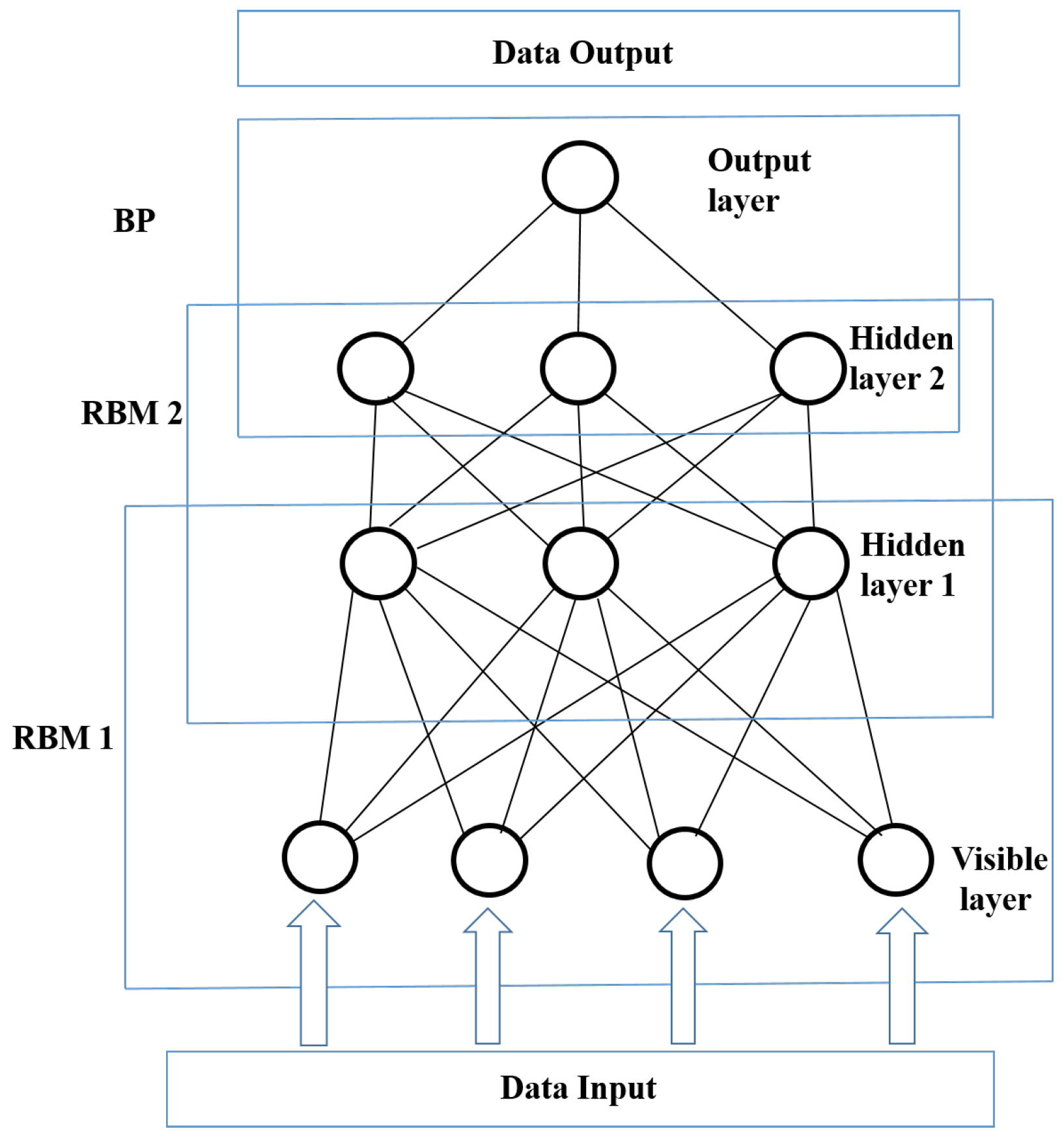
A DBN is a probabilistic generative model that consists of multiple hidden layers. The multiple layers can be used to learn more complex patterns of data in a progressive manner from low-level features to high-level features. One important feature of the learning algorithm for a DBN is that of its greedy layer-wise training, which can be repeated several times to efficiently learn a deep hierarchical model [38]. Other key features of DBN models include their ability to efficiently learn from large amounts of unlabeled data that can be discriminatively fine-tuned for classification and regression problems using the standard backpropagation algorithm [38]. They can also be used to make nonlinear autoencoders that work considerably better than standard feature reduction methods, such as principal component analysis (PCA) and singular value decomposition (SVD) [22,38]. A DBN is constructed by stacking multiple RBMs on top of each other [18,35]. The structure of a DBN with two RBMs is shown in Figure 3. The layers are trained efficiently by using the feature activations of one layer as the training data for the next layer. Better initial values of weights in all layers can be obtained by the layer-wise unsupervised training, compared to random initialization [18]. A DBN is trained using two steps: pre-training and fine-tuning. First, unsupervised pre-training is performed layer by layer, from low-level to high-level RBMs, to obtain reasonable parameter values of the network. Second, the entire network is fine-tuned in a supervised manner according to the target value using back-propagation.
Training a DBN is simply done by training the individually stacked RBMs constituting the network. An RBM is trained using contrastive divergence, which is an algorithmic procedure for the efficient estimation of RBM parameters. A standard way of estimating the RBM’s parameters from a training set with respect to a given weight is carried out by finding the parameters that maximize the average log probability.
where expresses the distribution of raw data input to the RBM, and is the distribution of data after the model has been reconstructed.
This can be summarized in the following few steps:
- set initial states to the training data set (visible units);
- sample in a back-and-forth process
- update all of the hidden units in parallel starting with visible units, reconstruct visible units from the hidden units, and finally update the hidden units again;
- repeat with all training examples and update the weights using Equation (9).
2.3. Empirical Mode Decomposition
EMD is a signal preprocessing algorithm that was introduced by Huang et al. in 1998 [27]. EMD is an adaptive data processing method that can be used for the decomposition of both nonlinear and nonstationary time series and has found applications in various domains. The method was developed based on the assumption that any time series data consists of different simple intrinsic modes of oscillation, i.e., IMFs. The essence of EMD is to empirically identify these intrinsic oscillatory modes by their characteristic time scales in the data and then decompose the data accordingly. It converts an irregular signal into a stationary signal process by continuously eliminating the average envelope of the sequence, thereby making the sequence smooth. It considers oscillations of the signal at a very local level and separates the signal into locally non-overlapping, zero-mean, stationary time scale components through a sifting process. The advantage of EMD over other signal decomposition techniques is that it does not need to be constrained by conditions, which often only apply approximately. Several hybrid models based on the principle of ‘decomposition and ensemble’ have been proposed. For instance, hybrid forecast approaches have been applied in hydrology research, as shown in [26,39,40,41]. A wavelet transform technique with ANN was employed in [39] and [40] to predict rainfall and streamflow time series respectively. In [41], Sang developed a method for discrete wavelet decomposition of time series and proposed an improved wavelet model for hydrologic time series forecasting. The results of these studies have proven that the ‘decomposition and ensemble’ principle-based forecasting methods can reduce the difficulty of forecasting and can outperform the single models [26]. Unlike wavelet transforms that have been widely used as decomposition techniques, EMD is a heuristic technique that is based on the properties of the data on a local scale. It decomposes the time series without the need of an a-priori-defined basis function in which the signal is expressed [27].
The necessary conditions of the IMFs are symmetry with respect to the local zero mean and the same number of zero crossings and extrema [27]. In order for an EMD to decompose a signal into the different IMFs, the following two properties must be met:
- an IMF has only one extremum between two subsequent zero crossings—i.e., the number of local extrema and zero crossings differs at most by one;
- the local average of the upper and lower envelopes of an IMF has to be zero.
The sifting process locally filters pure oscillations, starting with the highest frequency oscillation in an iterative procedure [27]. Hence, the sifting algorithm decomposes a data set into IMFs, where and a residue as shown in the following equation [42]. A more detailed procedure on how IMFs are calculated can be found in Wu et al. [42].
where represents the IMF components, and is a residual component. The residual could be a constant, or a function that contains only a single extrema and from which no more oscillatory IMFs can be extracted [42].
2.4. The EMD Algorithm
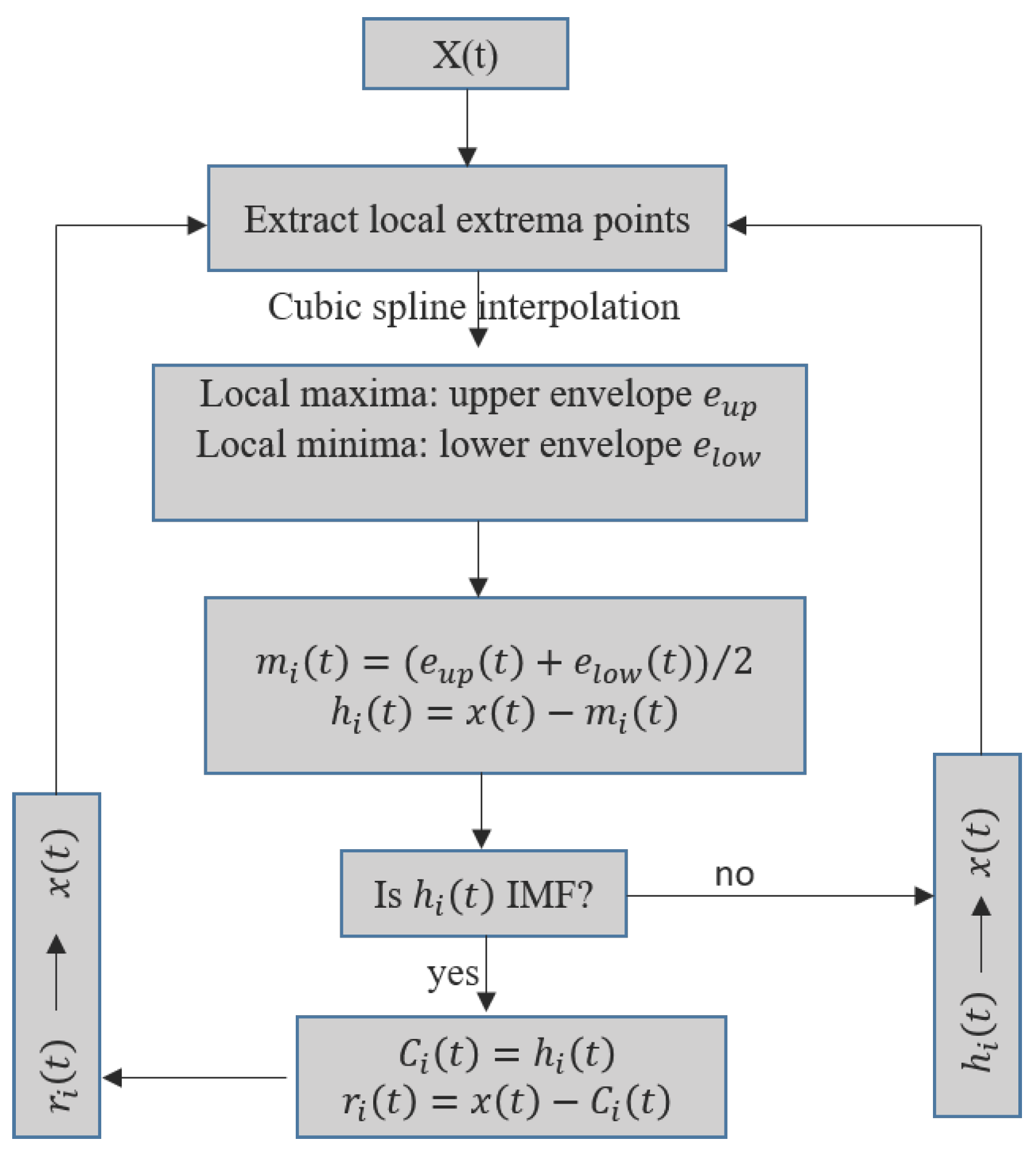
At the beginning of the proposed hybrid model, the EMD-based decomposition is employed to decompose the original signal into the various components. The main steps followed in the time series decomposition using EMD are as follows:
- identify all of the local extrema of ;
- create the upper envelope and the lower envelope by the cubic spline interpolation, respectively;
- compute the mean value of the upper and lower envelopes: ;
- extract the mean envelope from the signal , where the difference is defined as : ;
- check the properties of :
- (a)
- if d(t) satisfies the requirements of IMF Conditions (1) and (2), then is denoted as the ith IMF, and is replaced with the residual ; the ith IMF is denoted as , and i is the order number of the IMF;
- (b)
- if is not an IMF, replace with ;
- repeat Steps 1–5 until the residue becomes a monotonic function or the number of extrema is less than or equal to one, from which no further IMF can be extracted.
2.5. Detrended Fluctuation Analysis
Detrended fluctuation analysis (DFA) is a method proposed by Peng et al. [33] for measuring the intensity of the long-range dependence of a signal. This dependence can be described using three different classes: long-range dependence, mild dependence, and pure randomness. It can be used to estimate the scaling exponent of a signal that describes its self-affinity similarly to the Hurst exponent. The oldest and best-known method for estimation of the Hurst exponent is the so-called R/S analysis method, proposed by Mandelbrot and Wallis [32]. This method was first based on a previous work by Hurst on hydrological analysis that allows for the estimation of the Hurst exponent (self-similarity parameter H). However, the method is not suitable for nonstationary time series, as it can cause spurious scores [43]. In this work, detrended fluctuation analysis, which is a more suitable method for obtaining reliable scaling exponents for nonstationary time series is employed [32,43]. The method can be summarized as follows:
- for a given time series with length L, divide it into d subseries of length n;
- for each subseries ,
- (a)
- Create a cumulative time series for
- (b)
- Fit a least squares line to {}
- (c)
- Calculate the root mean square fluctuation (i.e. standard deviation) of the integrated and detrended time series:
- (d)
- Finally, calculate the mean value of the root mean square fluctuation for all subseries of length n
Similarly to the R/S analysis, a linear relationship on a double-logarithmic of against the interval size n indicates the presence of a power-law scaling behavior [32]. Here, H is the DFA scaling exponent that is identical to the Hurst exponent. The Hurst exponent is related to the power spectrum exponent and the autocorrelation exponent by and [44]. It is considered an indicator of the roughness of the time series. The larger the value, the smoother the time series. Smaller slope values are usually associated with rapid fluctuations. If the process is white noise, then the slope is roughly 0.5. If it is persistent, the slope is >0.5. If it is anti-persistent, the slope is <0.5. In such cases, significant fluctuations are followed by small ones and vice versa. Just like the R/S analysis approach, a drawback of the DFA is that no known asymptotic distribution theory has been derived from the statistics. As such, no explicit hypothesis testing can be performed, as the significance relies on a subjective assessment [32].
2.6. EMD-Based Denoising Using DFA
The EMD algorithm decomposes any complicated dataset into a finite number of IMFs of different dominant frequencies and amplitudes. The decomposed IMFs are usually arranged starting with the highest frequencies at the top and those with the lowest frequencies at the bottom. The original dataset can be reconstructed accurately by using all of the IMFs. However, some of the components, especially those with the highest frequencies, may contain irrelevant information about the original data (noise); therefore, using all the IMFs for reconstruction of the original dataset may affect the performance of any prediction method. A new series of the original dataset can be suitably reconstructed by using only a subset of the IMFs. This can be achieved by properly eliminating those IMFs that contain no relevant information about the original series. Different EMD-based denoising methods have been proposed and applied in various studies for different purposes [29,30]. An important step in EMD-based denoising is how to separate the noisy IMFs from the rest of the IMFs. A common method for EMD-based denoising algorithms is to eliminate the noise by using one of the IMF components. However, the decision as to which IMF to eliminate is still an ongoing research problem [31]. In this work, we propose a denoising approach that eliminates the noisy IMFs by using DFA to estimate the scaling exponents of all the IMFs and comparing them with the Hurst exponent threshold. The proposed method eliminates both Gaussian white noise and anti-persistent processes by using a Hurst exponent threshold of 0.5. A plot of the scaling exponents of the IMFs with a threshold of 0.5 is shown in Figure 6. The original dataset is therefore reconstructed by summing those IMFs with scaling exponents above the threshold. Figure 7 shows a plot of the original and the reconstructed dataset.
3. Study Area and Observed Dataset
3.1. Study Area
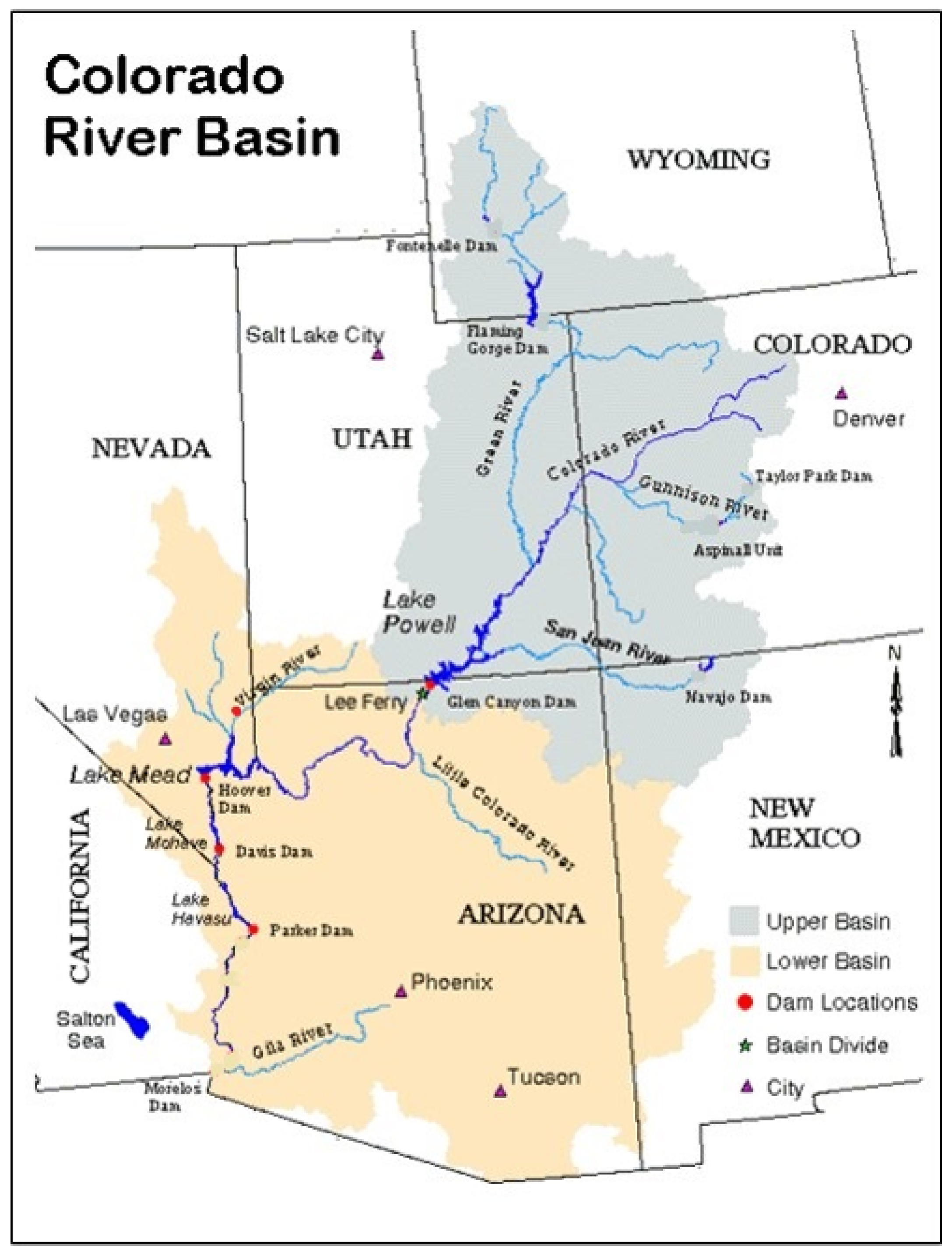
The study area is the Lower Colorado River Basin, shown in Figure 8 (credit: http://web.mit.edu/12.000/www/m2012/finalwebsite/images/col1.jpg). Ten river sites were used in this analysis and include the Colorado River and Paria River at Lee’s Ferry Basin, the Little Colorado River at Cameron, the Virgin River at Littlefield, the Colorado River below the Hoover Dam, the Colorado River below Davies Dam, the Colorado River near Grand Crayon, the Williams River below Alamo, the Colorado River below Parker Dam, and the Colorado River above Imperial Dam. Monthly natural streamflows for the period 1906 to 2014 were used to illustrate the proposed hybrid EMD-based predictive DBN. This monthly data is from the United States Geological Survey (USGS) observed gage data that can be obtained from the website of the Upper Colorado Regional Office of the United States Bureau of Reclamation at Salt Lake City, Utah (http://www.usbr.gov/lc/region/g4000/NaturalFlow/index.html). For long-term drought analysis and prediction, the 12-month and 24-month drought index scales are normally used. As a preliminary experiment, the 12-month scale SSI was used as the drought index.
3.2. Standardized Streamflow Index
We followed the concept employed by McKee et al. for the standardized precipitation index (SPI) [45] to calculate the SSI. Generally, drought indicators that are defined like the SPI are called standardized indices (SIs). McKee et al. used the Gamma distribution for fitting monthly precipitation data series and suggested that the procedure can be applied to variables other than precipitation, provided they are relevant to drought (for instance, streamflow, snowpack, and soil moisture) [45]. The procedure used by Cacciamani et al. [46] was followed in order to calculate the SSI. First, we modeled the distribution frequency of the total streamflow time series cumulated over different time scales (e.g., 3 months, 6 months, and 12 months) using a probability density function. Then, the probability density function was transformed into a normal standardized distribution. The values of the resulting standardized index could then be used to classify the category of drought characterizing each place and time scale [46]. Madadgar et al. [11] used a similar procedure to characterize the hydrological droughts of the Gunnison River Basin. Since the SSIs are calculated over different streamflow accumulation periods and scales, they can be used to estimate various potential impacts of a hydrological drought. For instance, the 12-month SSI shows a comparison of the streamflow for 12 consecutive months against the same 12 consecutive months of all the available data from previous years. A drought event is said to occur when the SSI is continuously negative for a certain period of time. The event is said to end when the index becomes positive. The SSI 12 and SSI 24 monthly scale drought indices are often tied to long-term drought conditions. Longer-term drought forecasts can serve as useful information about drought conditions that affect streamflow, groundwater, or other hydrological systems within the Colorado River basin.
3.3. Feature Extraction
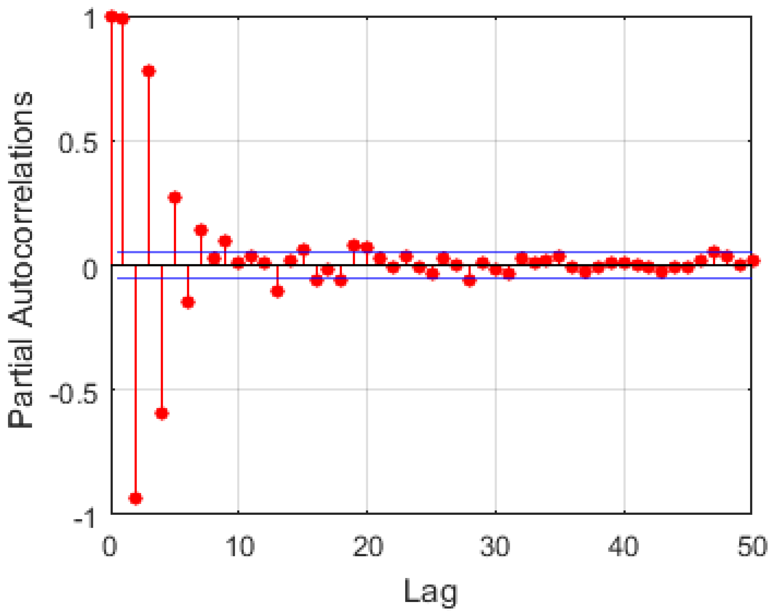
For time series prediction, the prediction is usually carried out using previous values of the series as features for the training model. The selection is based on their correlation with the output variable. In this work, the number of input neurons was selected using autocorrelation analysis. An example is illustrated in Figure 9 with lags of 1–7,9,13 showing different high levels of significance to the output. Based on the significance levels of the individual lags and experimentation, a lag of 6 was chosen. Hence, the past five observations and the current value () were used as inputs to predict the next observation (), as illustrated in Figure 10. These were somehow different for the various stations. For long-term targets, a recursive procedure was employed. The models were used to predict one step ahead, and the outputs from these models were used as inputs for subsequent predictions.
3.4. Evaluation of Model Performances
Although the Pearson correlation coefficient (r) and the coefficient of determination () have been widely used for model evaluation, they have been identified as inappropriate performance metrics for hydrological models [47,48]. They are oversensitive to extreme values and insensitive to additive and proportional differences between model predictions and observed data [48,49]. In order to have a complete assessment of model performance, Legates et al. [49] suggested that at least one absolute error measure, such as root mean square error (RMSE), mean absolute error (MAE) or mean absolute percentage error (MAPE), be included as performance metrics. Additionally, the Nash Sutcliffe model efficiency coefficient (NSE) [50] is a good alternative to r or [47]. Hence, the following three metrics were used for model comparison:
where is the observed data, represents the predicted values, is the mean of the observed data, and T is the length of the data.
3.5. Summary of the Proposed EMD based Predictive Deep Belief Network
The proposed EMD-based Predictive DBN consists of four main steps: (1) EMD decomposition of data into a finite number of IMFs; (2) noise reduction based on partial reconstruction using only the relevant IMFs; (3) DBN modeling and training; and (4) prediction using the trained model. A flowchart of the proposed approach is shown in Figure 11. Two RBMs were used to construct the DBN. The DBN model is therefore made of one visible (input) layer, two hidden layers, and a final layer (output) for fine-tuning the entire network as shown in Figure 3. Only two hidden layers (two stacked RBMs) were used to construct the DBN model because of the small data sample size. Higher hidden layer sizes were experimented but they were found to be over-fitting. The use of other meteorological variables as features in addition to the SSI may increase data size, and this may also necessitate the use of larger network sizes. The following few steps summarize the procedure of the proposed method:
- obtain the different time-scale SSI (SSI 12 in this case);
- decompose the time series data into several IMFs and a residue (Rn) using EMD;
- reconstruct the original data using only relevant IMF components;
- divide the data into training and testing sets (80% for training and 20% for testing);
- construct one training matrix as the input for the DBN;
- select the appropriate model structure and initialize the parameters of the DBN (two hidden layers are used);
- using the training data, pre-train the DBN through unsupervised learning;
- fine-tune the parameters of the entire network using the back-propagation algorithm;
- perform predictions with the trained model using the test data.
Because a typical RBM uses binary logistic units for visible nodes, we modified the binary nodes to the continuous case in order to handle the SSI continuous-valued input data using the technique presented in [18]. We rescaled the continuous-valued input data to the (0,1) interval and considered each continuous input value as the probability for a binary random variable to take the value 1. The transformation is given by:
where .
4. Results
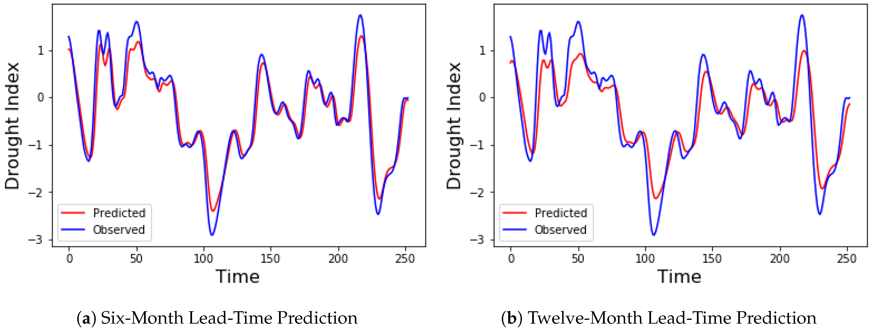
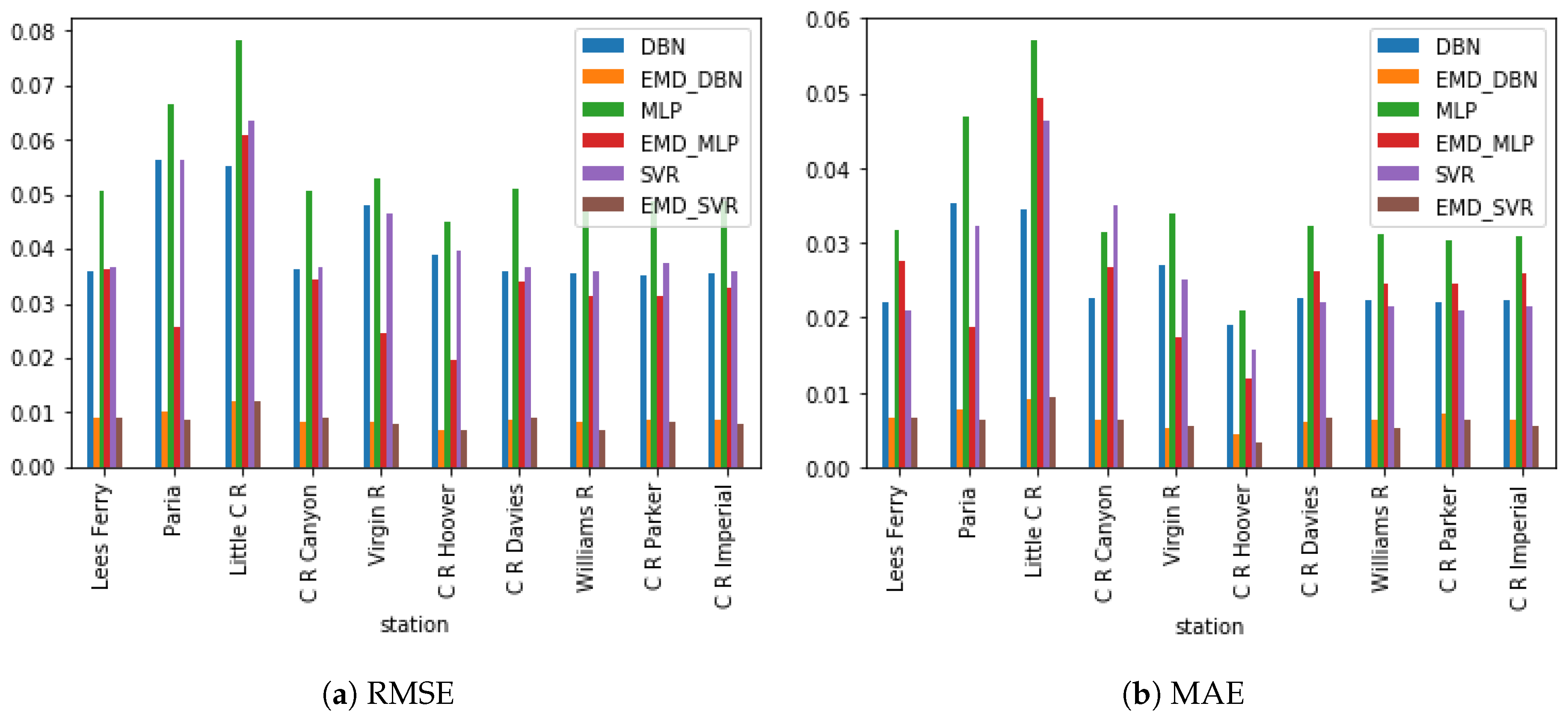
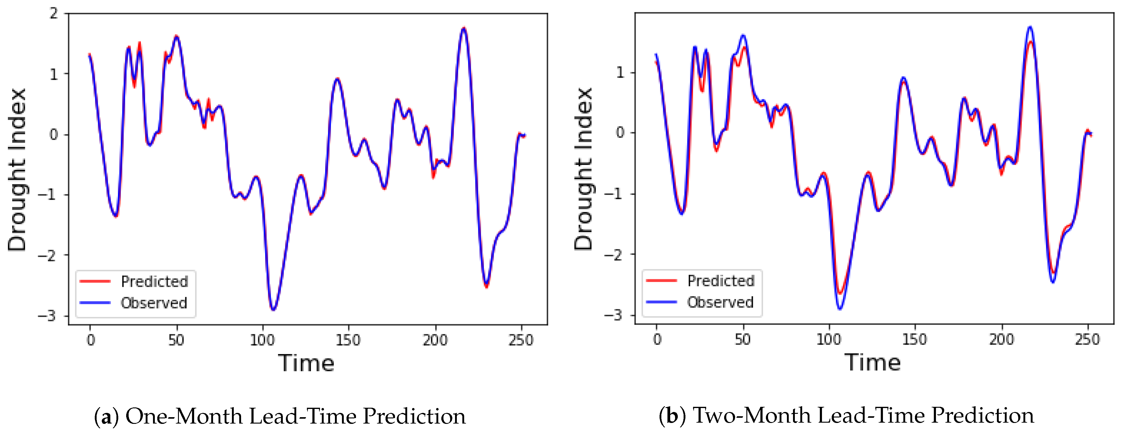
The proposed denoising EMD-based predictive DBN was evaluated by applying it to predict drought indices of different lead times across the Colorado River Basin. Standardized streamflow index (SSI) was used as the drought index. The forecast errors for predicting SSI 12 one-step-ahead (one-month lead time) and two-step-ahead (two-month lead time) for the chosen ten stations are presented in Table 1 and Table 2. Six models were compared. They include the MLP, SVR, the DBN, and the hybrid versions of these three models using EMD-DFA decomposition. Decomposition and denoising significantly improved the performance of the three models, with both DBN and SVR showing a performance far superior to that of MLP. Optimal parameters for both MLP and SVR were obtained using grid search on the training part of the dataset. Three performance metrics were used to compare the various models: the RMSE, the MAE, and the NSE. A histogram showing the RMSE and MAE for the one-step-ahead predictions are shown in Figure 12. The accuracies of both DBN and SVR are similar for most of the stations in the one-step-ahead prediction. However, in the two-step-ahead prediction, EMD-DBN outperforms the other models, as it recorded the least prediction errors in all stations as shown in Table 2. These results emphasize the importance of the unsupervised pretraining of neural networks using DBN over traditional neural networks. Figure 13 shows the one-month and two-month lead times forecasts for Lee’s Ferry station. Results of six-month and twelve-month lead times forecasts are also shown in Figure 14, where it can clearly be observed that the accuracy of prediction decreases as the prediction horizon increases.
5. Conclusions
Drought modeling and prediction has been a topic of interest over the last two decades, generating interest among researchers around the globe. In order to understand future drought event behavior, modeling of drought indices is very important. This study explored a DBN for drought prediction. We proposed a hybrid model (EMD-DBN) for long-term drought prediction. The results were compared with DBN, MLP, and SVR alone and with EMD-MLP and EMD-SVR. Overall, both DBN and SVR and their hybrid versions, showed comparatively similar prediction errors for the one-step ahead predictions as shown in Table 1 . However, DBN and the proposed EMD-DBN outperformed all other models for the two-step predictions for almost all stations, as shown in Table 2. Though the performance of MLP improved with the decomposition and denoising of drought indices, its performance, relative to both DBN and SVR was poor. In all, the improvement in the performance of the hybrid models over the single models suggests that errors encountered in time series predictions can be improved significantly by series decomposition using EMD. Pre-processing the original input dataset with EMD decreases the complexities in the data, allowing the removal of noisy components and therefore improving prediction accuracy. For long-term predictions, it was observed that, as the prediction horizon increases, the accuracy of predictions decreases. This was not unexpected because a recursive approach was employed for higher prediction lead times, where previous predictions were used as inputs for lead times greater than one. The results obtained from this work are very promising and pave the way for further works where hybrid models involving empirical mode decomposition techniques with future selection and other temporal models such as recurrent neural networks or variants can be explored. Additionally, due to the good performance of the SVR model, future work may try to employ the SVR as the last layer of the DBN pretrained model. Optimal parameter search for SVR can be improved by considering evolutionary optimization algorithms such as genetic algorithms (GAs) or PSO. This is necessary because the grid search method used in this work may be sensitive to the selected SVR parameters and might have influenced the results.
Future work will also consider the use of other meteorological variables such as precipitation, temperature, and large climate variables such as El Nino southern oscillation (ENSO) and North Atlantic oscillation (NAO) [51]. Drought is a very complex natural phenomenon, as it is known to be influenced by several meteorological variables. Hence, the use of only one variable may not be adequate enough to provide reliable forecasts. Additionally, climate change effects are very diverse. They vary both locally and regionally, in their intensity, duration, and areal extent. Hence, in order to understand the impact of climate change on drought, GCM outputs are downscaled to model drought variables on a large scale [17]. Therefore, we will try to adopt this current work to GCM or RCM outputs to assess drought characteristics.
Acknowledgments
This work was partially supported by the Expeditions in Computing by the National Science Foundation under Award Number CCF-1029731, and by the Air Force Research Laboratory and OSD under agreement number FA8750-15-2-0116. The U.S. Government is authorized to reproduce and distribute reprints for governmental purposes notwithstanding any copyright notation thereon. The views and conclusions contained herein are those of the authors and should not be interpreted as necessarily representing the official policies or endorsements, either expressed or implied, of NSF, Air Force Research Laboratory, OSD, or the U.S. Government.
Author Contributions
Both authors, Norbert A. Agana and Abdollah Homaifar contributed equally to the successful completion of this work.
Conflicts of Interest
The authors declare no conflict of interest.
References
- Wilhite, D.A.; Hayes, M.J. Drought planning in the united states: Status and future directions. In The Arid Frontier; Springer: Dordrecht, The Netherlands, 1998; pp. 33–54. [Google Scholar]
- Morid, S.; Smakhtin, V.; Bagherzadeh, K. Drought forecasting using artificial neural networks and time series of drought indices. Int. J. Climatol. 2007, 27, 2103–2111. [Google Scholar] [CrossRef]
- Smith, A.B.; Katz, R.W. Us billion-dollar weather and climate disasters: Data sources, trends, accuracy and biases. Nat. Hazards 2013, 67, 387–410. [Google Scholar] [CrossRef]
- Changnon, S.A.; Pielke, R.A., Jr.; Changnon, D.; Sylves, R.T.; Pulwarty, R. Human factors explain the increased losses from weather and climate extremes. Bull. Am. Meteorol. Soc. 2000, 81, 437. [Google Scholar] [CrossRef]
- Ross, T.; Lott, N. A Climatology of 1980–2003 Extreme Weather and Climate Events; US Department of Commerece, National Ocanic and Atmospheric Administration, National Environmental Satellite Data and Information Service, National Climatic Data Center: Asheville, NC, USA, 2003.
- Nielsen-Gammon, J.W. The 2011 texas drought. Texas Water J. 2012, 3, 59–95. [Google Scholar]
- Hoerling, M.; Eischeid, J.; Kumar, A.; Leung, R.; Mariotti, A.; Mo, K.; Schubert, S.; Seager, R. Causes and predictability of the 2012 great plains drought. Bull. Am. Meteorol. Soc. 2014, 95, 269–282. [Google Scholar] [CrossRef]
- Griffin, D.; Anchukaitis, K.J. How unusual is the 2012–2014 california drought? Geophys. Res. Lett. 2014, 41, 9017–9023. [Google Scholar] [CrossRef]
- Dutra, E.; Magnusson, L.; Wetterhall, F.; Cloke, H.L.; Balsamo, G.; Boussetta, S.; Pappenberger, F. The 2010–2011 drought in the horn of africa in ecmwf reanalysis and seasonal forecast products. Int. J. Climatol. 2013, 33, 1720–1729. [Google Scholar] [CrossRef]
- Hao, Z.; AghaKouchak, A.; Nakhjiri, N.; Farahmand, A. Global integrated drought monitoring and prediction system. Sci. Data 2014, 1, 140001. [Google Scholar] [CrossRef] [PubMed]
- Madadgar, S.; Moradkhani, H. A bayesian framework for probabilistic seasonal drought forecasting. J. Hydrometeorol. 2013, 14, 1685–1705. [Google Scholar] [CrossRef]
- Mishra, A.K.; Desai, V.R. Drought forecasting using feed-forward recursive neural network. Ecol. Model. 2006, 198, 127–138. [Google Scholar] [CrossRef]
- Mehr, A.D.; Kahya, E.; Özger, M. A gene–wavelet model for long lead time drought forecasting. J. Hydrol. 2014, 517, 691–699. [Google Scholar] [CrossRef]
- Belayneh, A.; Adamowski, J.; Khalil, B.; Ozga-Zielinski, B. Long-term spi drought forecasting in the awash river basin in ethiopia using wavelet neural network and wavelet support vector regression models. J. Hydrol. 2014, 508, 418–429. [Google Scholar] [CrossRef]
- Mishra, A.K.; Singh, V.P. A review of drought concepts. J. Hydrol. 2010, 391, 202–216. [Google Scholar] [CrossRef]
- Mishra, A.K.; Desai, V.R.; Singh, V.P. Drought forecasting using a hybrid stochastic and neural network model. J. Hydrol. Eng. 2007, 12, 626–638. [Google Scholar] [CrossRef]
- Mishra, A.K.; Singh, V.P. Drought modeling—A review. J. Hydrol. 2011, 403, 157–175. [Google Scholar] [CrossRef]
- Bengio, Y.; Lamblin, P.; Popovici, D.; Larochelle, H. Greedy layer-wise training of deep networks. Adv. Neural Inf. Process. Syst. 2007, 19, 153. [Google Scholar]
- Blenkinsop, S.; Fowler, H.J. Changes in drought frequency, severity and duration for the british isles projected by the prudence regional climate models. J. Hydrol. 2007, 342, 50–71. [Google Scholar] [CrossRef]
- Chun, K.P.; Wheater, H.; Onof, C. Prediction of the impact of climate change on drought: an evaluation of six uk catchments using two stochastic approaches. Hydrol. Processes 2013, 27, 1600–1614. [Google Scholar] [CrossRef]
- Liu, T. A novel text classification approach based on deep belief network. In Proceedings of the International Conference on Neural Information Processing, Sydney, Australia, 22–25 November 2010; Springer: Berlin, Germany, 2010; pp. 314–321. [Google Scholar]
- Hinton, G.E.; Salakhutdinov, R.R. Reducing the dimensionality of data with neural networks. Science 2006, 313, 504–507. [Google Scholar] [CrossRef] [PubMed]
- Zhang, R.; Shen, F.; Zhao, J. A model with fuzzy granulation and deep belief networks for exchange rate forecasting. In Proceedings of the 2014 International Joint Conference on Neural Networks (IJCNN), Beijing, China, 6–11 July 2014; pp. 366–373. [Google Scholar]
- Chen, J.; Jin, Q.; Chao, J. Design of deep belief networks for short-term prediction of drought index using data in the huaihe river basin. Math. Probl. Eng. 2012, 2012, 235929. [Google Scholar] [CrossRef]
- Kuremoto, T.; Kimura, S.; Kobayashi, K.; Obayashi, M. Time series forecasting using a deep belief network with restricted boltzmann machines. Neurocomputing 2014, 137, 47–56. [Google Scholar] [CrossRef]
- Di, C.; Yang, X.; Wang, X. A four-stage hybrid model for hydrological time series forecasting. PLoS ONE 2014, 9, e104663. [Google Scholar] [CrossRef] [PubMed]
- Huang, N.E.; Shen, Z.; Long, S.R.; Wu, M.C.; Shih, H.H.; Zheng, Q.; Yen, N.; Tung, C.C.; Liu, H.H. The empirical mode decomposition and the hilbert spectrum for nonlinear and non-stationary time series analysis. In Proceedings of the Royal Society of London A: Mathematical, Physical and Engineering Sciences; The Royal Society: London, UK, 1998; Volume 454, pp. 903–995. [Google Scholar]
- Labate, D.; la Foresta, F.; Occhiuto, G.; Morabito, F.C.; Lay-Ekuakille, A.; Vergallo, P. Empirical mode decomposition vs. wavelet decomposition for the extraction of respiratory signal from single-channel ecg: A comparison. IEEE Sens. J. 2013, 13, 2666–2674. [Google Scholar] [CrossRef]
- Premanode, B.; Vonprasert, J.; Toumazou, C. Prediction of exchange rates using averaging intrinsic mode function and multiclass support vector regression. Artif. Intell. Res. 2013, 2, 47. [Google Scholar] [CrossRef]
- Boudraa, A.O.; Cexus, J.C.; Saidi, Z. Emd-based signal noise reduction. Int. J. Signal Process. 2004, 1, 33–37. [Google Scholar]
- Yaslan, Y.; Bican, B. Empirical mode decomposition based denoising method with support vector regression for time series prediction: A case study for electricity load forecasting. Measurement 2017, 103, 52–61. [Google Scholar] [CrossRef]
- Weron, R. Estimating long-range dependence: Finite sample properties and confidence intervals. Phys. A Stat. Mech. Appl. 2002, 312, 285–299. [Google Scholar] [CrossRef]
- Peng, C.-K.; Buldyrev, S.V.; Havlin, S.; Simons, M.; Stanley, H.E.; Goldberger, A.L. Mosaic organization of dna nucleotides. Phys. Rev. E 1994, 49, 1685. [Google Scholar] [CrossRef]
- Tieleman, T. Training restricted boltzmann machines using approximations to the likelihood gradient. In Proceedings of the 25th International Conference on Machine Learning, Helsinki, Finland, 5–9 July 2008; ACM: New York, NY, USA, 2008; pp. 1064–1071. [Google Scholar]
- Hinton, G.E.; Osindero, S.; Teh, Y.-W. A fast learning algorithm for deep belief nets. Neural Computat. 2006, 18, 1527–1554. [Google Scholar] [CrossRef] [PubMed]
- Agana, N.A.; Homaifar, A. A deep learning based approach for long-term drought prediction. In Proceedings of the SoutheastCon, Charlotte, NC, USA, 30 March–2 April 2017; pp. 1–8. [Google Scholar]
- Agana, N.A.; Homaifar, A. A hybrid deep belief network for long-term drought prediction. In Proceedings of the Workshop on Mining Big Data in Climate and Environment (MBDCE 2017), 17th SIAM International Conference on Data Mining (SDM 2017), Houston, TX, USA, 27–29 April 2017; pp. 1–8. [Google Scholar]
- Salakhutdinov, R. Learning deep generative models. Annu. Rev. Stat. Appl. 2015, 2, 361–385. [Google Scholar] [CrossRef]
- Kisi, O. Wavelet regression model for short-term streamflow forecasting. J. Hydrol. 2010, 389, 344–353. [Google Scholar] [CrossRef]
- Nourani, V.; Komasi, M.; Mano, A. A multivariate ann-wavelet approach for rainfall–runoff modeling. Water Resour. Manag. 2009, 23, 2877. [Google Scholar] [CrossRef]
- Sang, Y.-F. Improved wavelet modeling framework for hydrologic time series forecasting. Water Resour. Manag. 2013, 27, 2807–2821. [Google Scholar] [CrossRef]
- Wu, Z.; Huang, N.E.; Long, S.R.; Peng, C. On the trend, detrending, and variability of nonlinear and nonstationary time series. Proc. Natl. Acad. Sci. USA 2007, 104, 14889–14894. [Google Scholar] [CrossRef] [PubMed]
- Mert, A.; Akan, A. Detrended fluctuation thresholding for empirical mode decomposition based denoising. Dig. Signal Process. 2014, 32, 48–56. [Google Scholar] [CrossRef]
- Qian, X.; Gu, G.; Zhou, W. Modified detrended fluctuation analysis based on empirical mode decomposition for the characterization of anti-persistent processes. Phys. A Stat. Mech. Appl. 2011, 390, 4388–4395. [Google Scholar] [CrossRef]
- McKee, T.B.; Doesken, N.J.; Kleist, J. The relationship of drought frequency and duration to time scales. In Proceedings of the 8th Conference on Applied Climatology, Boston, MA, USA, 17–22 January 1993; American Meteorological Society Boston: Boston, MA, USA, 1993; Volume 17, pp. 179–183. [Google Scholar]
- Cacciamani, C.; Morgillo, A.; Marchesi, S.; Pavan, V. Monitoring and forecasting drought on a regional scale: Emilia-romagna region. In Methods and Tools for Drought Analysis and Management; Springer: Dordrecht, The Netherlands, 2007; pp. 29–48. [Google Scholar]
- Wu, C.L.; Chau, K.W.; Fan, C. Prediction of rainfall time series using modular artificial neural networks coupled with data-preprocessing techniques. J. Hydrol. 2010, 389, 146–167. [Google Scholar] [CrossRef]
- Moriasi, D.N.; Arnold, J.G.; van Liew, M.W.; Bingner, R.L.; Harmel, R.D.; Veith, T.L. Model evaluation guidelines for systematic quantification of accuracy in watershed simulations. Trans. ASABE 2007, 50, 885–900. [Google Scholar] [CrossRef]
- Legates, D.R.; McCabe, G.J. Evaluating the use of “goodness-of-fit” measures in hydrologic and hydroclimatic model validation. Water Resour. Res. 1999, 35, 233–241. [Google Scholar] [CrossRef]
- Nash, J.E.; Sutcliffe, J.V. River flow forecasting through conceptual models part i—A discussion of principles. J. Hydrol. 1970, 10, 282–290. [Google Scholar] [CrossRef]
- Moreira, E.E.; Pires, C.L.; Pereira, L.S. Spi drought class predictions driven by the north atlantic oscillation index using log-linear modeling. Water 2016, 8, 43. [Google Scholar] [CrossRef]
Figure 1.
An example of a restricted Boltzmann machine (RBM).
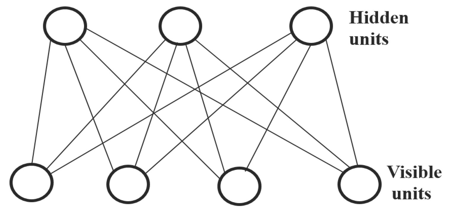
Figure 2.
A single step of contrastive divergence.
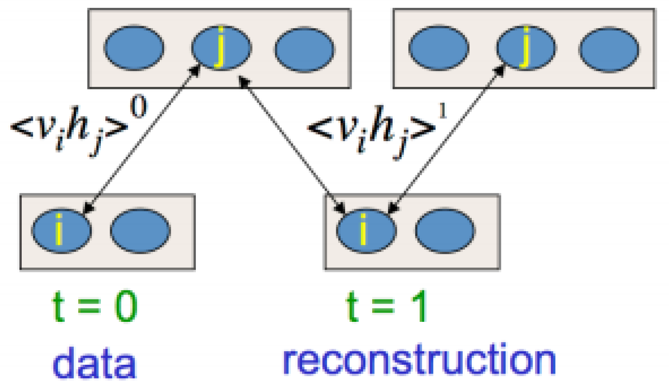
Figure 3.
Architecture of a deep belief network (DBN) with two RBMs [37].
Figure 3.
Architecture of a deep belief network (DBN) with two RBMs [37].

Figure 4.
Flowchart of the sifting process for the empirical mode decomposition (EMD) algorithm.

Figure 5.
Decomposition using EMD.
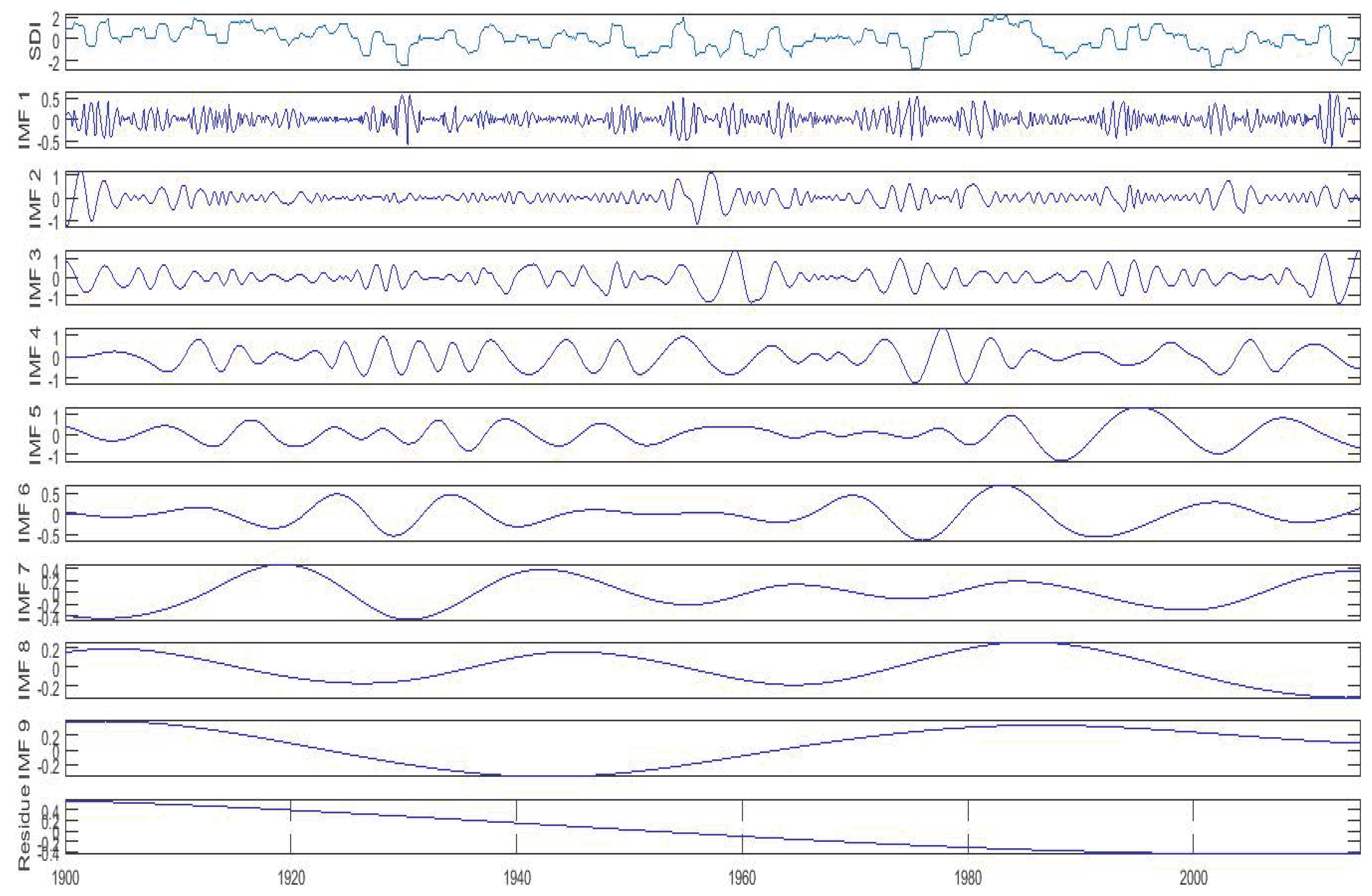
Figure 6.
Scaling exponents of all intrinsic mode functions (IMFs) with a threshold of 0.5.
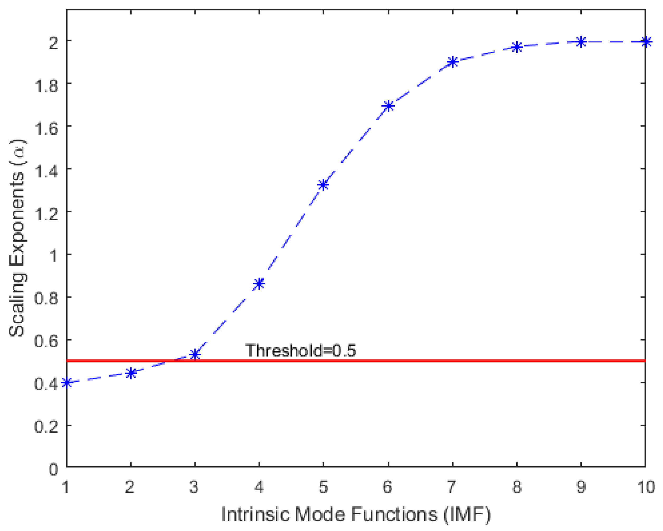
Figure 7.
A plot of the original and reconstructed dataset.
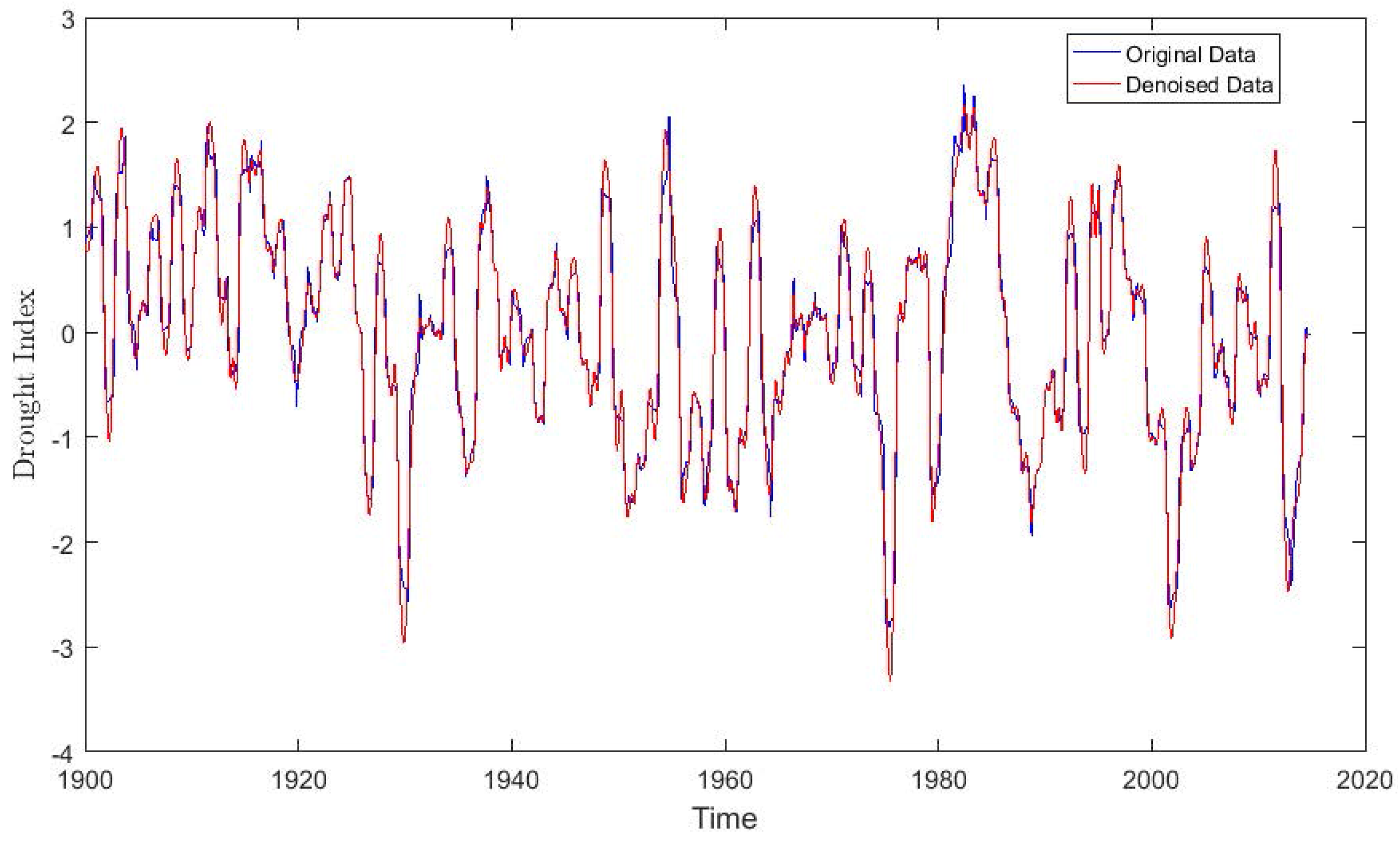
Figure 8.
Location of gages at the Colorado River near Lee’s Ferry, Paria River near Lee’s Ferry, Little Colorado River near Cameron, Virgin River near Littlefield, the Colorado River below the Hoover Dam, the Colorado River below Davies Dam, and the Colorado below Parker Dam (red dots).
Figure 8.
Location of gages at the Colorado River near Lee’s Ferry, Paria River near Lee’s Ferry, Little Colorado River near Cameron, Virgin River near Littlefield, the Colorado River below the Hoover Dam, the Colorado River below Davies Dam, and the Colorado below Parker Dam (red dots).

Figure 9.
Partial autocorrelation of features.

Figure 10.
An example of a recursive network.
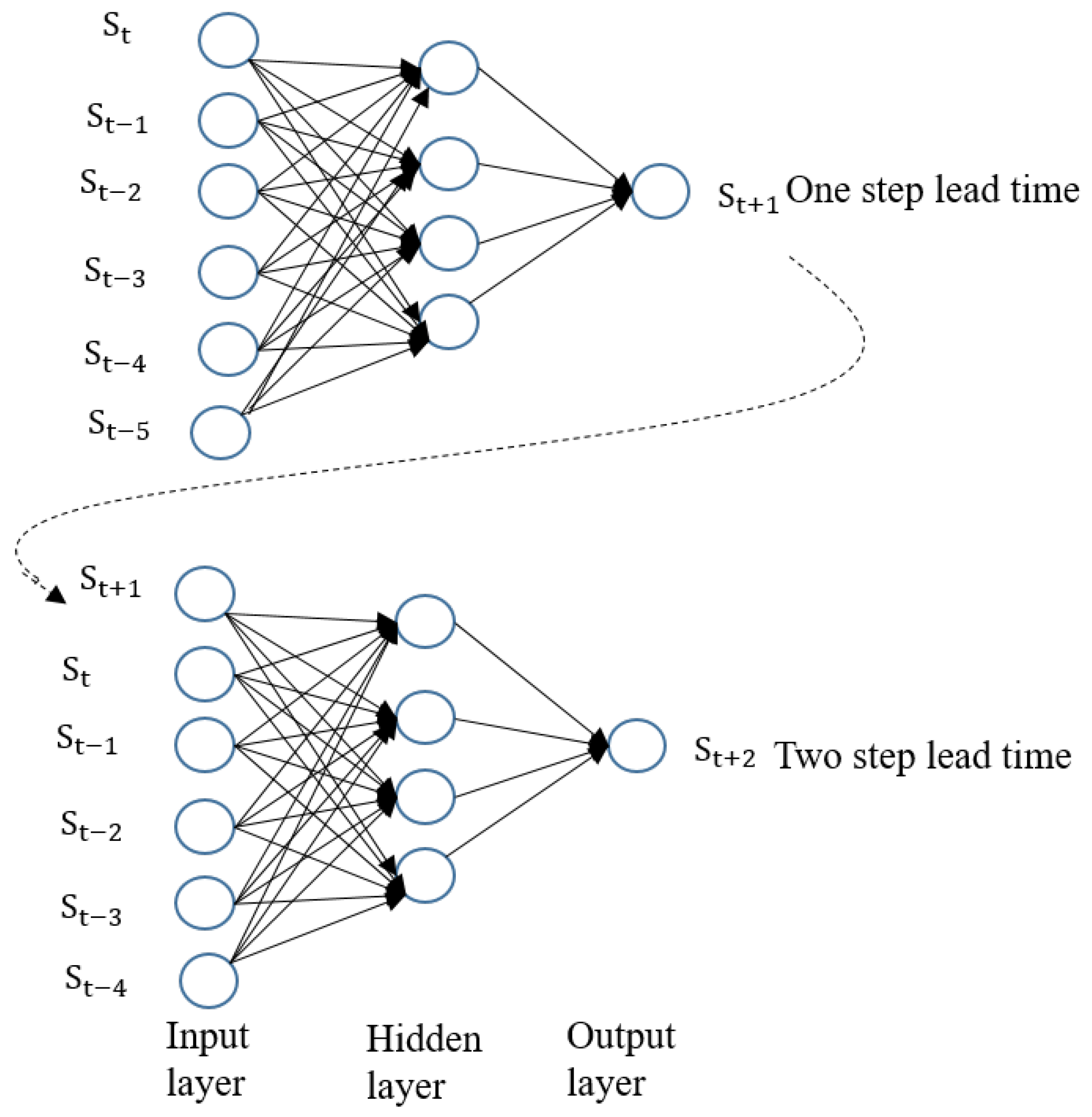
Figure 11.
Flowchart of the hybrid EMD-DBN model.

Figure 12.
Comparative plots of root mean square error (RMSE) and mean absolute error (MAE) for the various methods: one step ahead.
Figure 12.
Comparative plots of root mean square error (RMSE) and mean absolute error (MAE) for the various methods: one step ahead.

Figure 13.
Observed and predicted drought Index using the EMD-DBN model for Lee’s Ferry Station.

Figure 14.
Observed and predicted drought index using the EMD-DBN model for Lee’s Ferry Station.

Table 1.
Model results: one-step-ahead prediction.
| Station | Metric | DBN | EMD-DBN | MLP | EMD-MLP | SVR | EMD-SVR |
|---|---|---|---|---|---|---|---|
| Lee’s Ferry | RMSE | 0.03609 | 0.00892 | 0.05063 | 0.03638 | 0.03673 | 0.00918 |
| MAE | 0.022118 | 0.00647 | 0.03157 | 0.02745 | 0.02104 | 0.00667 | |
| NSE | 0.96323 | 0.99686 | 0.93207 | 0.96323 | 0.96504 | 0.99766 | |
| Paria | RMSE | 0.056349 | 0.0103 | 0.066744 | 0.025649 | 0.056196 | 0.008668 |
| MAE | 0.035205 | 0.007753 | 0.046733 | 0.018784 | 0.032271 | 0.006369 | |
| NSE | 0.89618 | 0.99655 | 0.84850 | 0.97231 | 0.89359 | 0.99683 | |
| Little C R | RMSE | 0.055215 | 0.0119 | 0.078347 | 0.060729 | 0.063625 | 0.012007 |
| MAE | 0.034330 | 0.00899 | 0.05710 | 0.049367 | 0.046197 | 0.00925 | |
| NSE | 0.87431 | 0.99408 | 0.81794 | 0.95161 | 0.86324 | 0.99403 | |
| C R Canyon | RMSE | 0.036122 | 0.00814 | 0.050631 | 0.034439 | 0.036642 | 0.009173 |
| MAE | 0.022646 | 0.006386 | 0.031531 | 0.026860 | 0.034869 | 0.006455 | |
| NSE | 0.96486 | 0.99853 | 0.93248 | 0.96803 | 0.96463 | 0.99842 | |
| Virgin R | RMSE | 0.048079 | 0.00817 | 0.053033 | 0.024385 | 0.046524 | 0.007942 |
| MAE | 0.027074 | 0.005180 | 0.033781 | 0.017263 | 0.025161 | 0.005616 | |
| NSE | 0.95914 | 0.99852 | 0.95262 | 0.98986 | 0.96421 | 0.99892 | |
| C R Hoover | RMSE | 0.038824 | 0.00686 | 0.045099 | 0.019594 | 0.039546 | 0.006937 |
| MAE | 0.018958 | 0.004499 | 0.021003 | 0.011846 | 0.015699 | 0.003347 | |
| NSE | 0.95193 | 0.99827 | 0.93280 | 0.98445 | 0.94833 | 0.99830 | |
| C R Davies | RMSE | 0.035912 | 0.00865 | 0.051219 | 0.034183 | 0.036535 | 0.008977 |
| MAE | 0.022693 | 0.006081 | 0.032272 | 0.026294 | 0.022015 | 0.006652 | |
| NSE | 0.96658 | 0.99722 | 0.93299 | 0.96613 | 0.96590 | 0.99780 | |
| Williams R | RMSE | 0.035366 | 0.00844 | 0.049666 | 0.03132 | 0.035801 | 0.006914 |
| MAE | 0.022378 | 0.006385 | 0.031253 | 0.024498 | 0.021475 | 0.005218 | |
| NSE | 0.96553 | 0.99748 | 0.93463 | 0.97234 | 0.96603 | 0.99801 | |
| C R Parker | RMSE | 0.035261 | 0.00875 | 0.048665 | 0.031484 | 0.037417 | 0.008185 |
| MAE | 0.022174 | 0.007089 | 0.030343 | 0.024622 | 0.021004 | 0.006305 | |
| NSE | 0.96085 | 0.99757 | 0.93435 | 0.96991 | 0.96451 | 0.99796 | |
| C R Imperial | RMSE | 0.035366 | 0.00844 | 0.049666 | 0.03132 | 0.035801 | 0.006914 |
| MAE | 0.022378 | 0.006385 | 0.031253 | 0.024498 | 0.021475 | 0.005218 | |
| NSE | 0.96245 | 0.99756 | 0.93617 | 0.96832 | 0.96540 | 0.99815 |
Table 2.
Model results: two-step-ahead prediction.
| Station | Metric | DBN | EMD-DBN | MLP | EMD-MLP | SVR | EMD-SVR |
|---|---|---|---|---|---|---|---|
| Lee’s Ferry | RMSE | 0.03760 | 0.01298 | 0.06858 | 0.04391 | 0.03830 | 0.01797 |
| MAE | 0.02314 | 0.01010 | 0.05181 | 0.03321 | 0.02454 | 0.01328 | |
| NSE | 0.95719 | 0.99540 | 0.87426 | 0.94605 | 0.96204 | 0.99118 | |
| Paria | RMSE | 0.05824 | 0.01177 | 0.07267 | 0.05547 | 0.05828 | 0.017298 |
| MAE | 0.04367 | 0.00924 | 0.05958 | 0.04810 | 0.04053 | 0.01344 | |
| NSE | 0.88405 | 0.99423 | 0.81943 | 0.87183 | 0.88386 | 0.98754 | |
| Little C R | RMSE | 0.06628 | 0.01693 | 0.07549 | 0.04769 | 0.07102 | 0.02833 |
| MAE | 0.04955 | 0.01332 | 0.06079 | 0.03727 | 0.04859 | 0.02094 | |
| NSE | 0.77706 | 0.98729 | 0.71083 | 0.89925 | 0.77409 | 0.96444 | |
| C R Canyon | RMSE | 0.03742 | 0.01114 | 0.06501 | 0.03640 | 0.03674 | 0.01447 |
| MAE | 0.02547 | 0.00815 | 0.04493 | 0.02718 | 0.03057 | 0.01067 | |
| NSE | 0.95384 | 0.99668 | 0.89088 | 0.95201 | 0.94519 | 0.99440 | |
| Virgin R | RMSE | 0.04420 | 0.01053 | 0.05337 | 0.03919 | 0.07664 | 0.03023 |
| MAE | 0.02765 | 0.00775 | 0.03703 | 0.03276 | 0.03963 | 0.01838 | |
| NSE | 0.94665 | 0.99810 | 0.92137 | 0.97376 | 0.89972 | 0.98438 | |
| C R Hoover | RMSE | 0.04997 | 0.01049 | 0.06616 | 0.04582 | 0.05298 | 0.02021 |
| MAE | 0.03089 | 0.00654 | 0.03266 | 0.04188 | 0.02707 | 0.01010 | |
| NSE | 0.89898 | 0.99483 | 0.82291 | 0.90135 | 0.88644 | 0.98080 | |
| C R Davies | RMSE | 0.03705 | 0.01395 | 0.05359 | 0.02945 | 0.04048 | 0.01529 |
| MAE | 0.02655 | 0.01060 | 0.03440 | 0.02330 | 0.02898 | 0.01128 | |
| NSE | 0.94084 | 0.99476 | 0.92770 | 0.97102 | 0.93875 | 0.99370 | |
| Williams R | RMSE | 0.033984 | 0.01035 | 0.06008 | 0.02838 | 0.03689 | 0.01502 |
| MAE | 0.02843 | 0.00780 | 0.03661 | 0.02559 | 0.02966 | 0.01119 | |
| NSE | 0.94899 | 0.99501 | 0.91175 | 0.95620 | 0.92468 | 0.99376 | |
| C R Parker | RMSE | 0.03713 | 0.01237 | 0.05935 | 0.02911 | 0.03905 | 0.01311 |
| MAE | 0.02493 | 0.00920 | 0.03715 | 0.02408 | 0.02535 | 0.01010 | |
| NSE | 0.93004 | 0.99538 | 0.90386 | 0.96657 | 0.92454 | 0.99480 | |
| C R Imperial | RMSE | 0.03601 | 0.01230 | 0.05998 | 0.02802 | 0.03729 | 0.01455 |
| MAE | 0.02424 | 0.00832 | 0.03834 | 0.02366 | 0.02590 | 0.01063 | |
| NSE | 0.94935 | 0.99561 | 0.90469 | 0.97006 | 0.95316 | 0.99386 |
© 2018 by the authors. Licensee MDPI, Basel, Switzerland. This article is an open access article distributed under the terms and conditions of the Creative Commons Attribution (CC BY) license (http://creativecommons.org/licenses/by/4.0/).
Share and Cite
MDPI and ACS Style
Agana, N.A.; Homaifar, A. EMD-Based Predictive Deep Belief Network for Time Series Prediction: An Application to Drought Forecasting. Hydrology 2018, 5, 18. https://doi.org/10.3390/hydrology5010018
AMA Style
Agana NA, Homaifar A. EMD-Based Predictive Deep Belief Network for Time Series Prediction: An Application to Drought Forecasting. Hydrology. 2018; 5(1):18. https://doi.org/10.3390/hydrology5010018
Chicago/Turabian StyleAgana, Norbert A., and Abdollah Homaifar. 2018. "EMD-Based Predictive Deep Belief Network for Time Series Prediction: An Application to Drought Forecasting" Hydrology 5, no. 1: 18. https://doi.org/10.3390/hydrology5010018
Note that from the first issue of 2016, this journal uses article numbers instead of page numbers. See further details here.