Generation of Spatially Heterogeneous Flood Events in an Alpine Region—Adaptation and Application of a Multivariate Modelling Procedure


1
alpS—Centre for Climate Change Adaptation, Grabenweg 68, 6020 Innsbruck, Austria
2
PPE Research Centre, Hochschulstrasse 1, 6850 Dornbirn, Austria
*
Author to whom correspondence should be addressed.
Hydrology 2018, 5(1), 5; https://doi.org/10.3390/hydrology5010005
Submission received: 15 November 2017
/
Revised: 21 December 2017
/
Accepted: 21 December 2017
/
Published: 4 January 2018
Abstract
:Flooding often has a negative impact on society. In particular, widespread flood events can cause a lot of damage. These events are often spatially and temporally heterogeneous and should be duly considered for an appropriate analysis of flooding. Therefore, a conditional multivariate approach is adapted and applied in order to (i) contribute to a better understanding of the spatial characteristics of fluvial floods and (ii) to deliver sets of synthetically generated flood events. The present paper focuses on a simulation procedure consisting of careful data preparation and selection and the application of a conditional multivariate approach. The conditional approach is adapted to account for the seasonality of runoff data. Model checks attuned to the model are presented to ensure the consistence of simulated and observed data. The Austrian Province Vorarlberg was chosen as the study area. A thorough data analysis of runoff time series showed that the hydrological behaviour is characterized by a strong seasonality that was considered within the applied modelling procedure. The analysis of the spatial dependence of high river flows identified regions where floods likely occur simultaneously and regions with low spatial dependence. The main result of the modelling procedure, a large set of widespread flood events, was successfully generated.
1. Introduction
Fluvial floods are a natural phenomenon that regularly cause significant losses to property and human life. Through efficient flood risk management, the adverse consequences of flooding can be mitigated or even avoided. Therefore, a thorough flood risk analysis provides the basis for decision making of involved parties, such as flood management agencies, public authorities, and insurance industries.
In this context, flood risk is usually understood as a combination of the probability of events and the potential adverse consequences [1,2,3]. A traditional procedure to derive the probability of flooding is to apply extreme value statistics to observed runoff series at river gauging stations. By means of this flood frequency analysis, the return period (T) of flood events in a year is determined for a single point i.e., gauging station) and being assigned to an entire catchment. In the course of flood risk analyses, these homogenous flood scenarios, assuming constant return periods of discharges within a river reach or an entire region, are frequently used.
As flood events in most cases are heterogeneous in space and time [4,5], the use of homogenous flood scenarios may lead to inaccurate results [6,7]. Therefore, heterogeneous flood scenarios, which take into account the spatial variability of flood events, should be considered in flood risk analysis [6,8,9]. As the number of past observed flood events leading to flood damages is usually low, the corresponding number of heterogeneous flood scenarios is limited and a statistical evaluation of the flood risk is difficult to achieve.
A promising approach to overcome this shortcoming is the simulation of synthetic flood events considering a vast range of possible flooding situations. The flood characteristics within a region of interest is typically represented by several gauging stations, and therefore a multivariate method, which is also capable of reproducing the spatial dependence structure in the investigated region, has to be applied.
In the field of hydrology, a popular approach to combine different marginal distributions and dependence structures is the copula approach. Although, in recent years, copula-based models have been applied in hydrology and related fields, such as multivariate frequency analysis, risk assessment, and multivariate extreme value analysis [8,10,11,12,13,14,15,16,17,18,19], most applications are limited to bivariate and trivariate cases. Jongman et al. [8] used a stepwise conditional copula approach to account for a higher dimensional case in flood risk analysis. Apart from this study, the semi-parametric conditional exceedance model introduced by Heffernan and Tawn [20] (henceforth referred to as the HT model) is able to capture the multivariate nature of widespread flooding and can be used to simulate flood events.
The HT model can be interpreted as a multisite peak-over-threshold approach [21] and is able to model the joint probability of large sets of variables (e.g., river flow or sea-level data). It is an appropriate model to describe the probability that one or multiple variables are extreme. Because of these properties, the HT model is well-suited (i) to show the dependence structure of runoff in a region and (ii) to describe and reproduce the joint occurrence of high river flows at different sites. The HT model, thus, delivers high and extreme runoff peaks at one or multiple sites representing heterogeneous flood situations. A key feature of the HT model is its flexibility in modeling different dependence structures of extreme events. It can be used for both asymptotically dependent and asymptotically independent data. None of these two dependence structures should be excluded by the applied model (as it is done e.g., by a copula model) because it is likely that, for example, two gauges along the same river are asymptotically dependent, whereas it is possible that not-nested sites are asymptotically independent. Furthermore, the HT model is able to describe the changing dependence structure when runoffs become extreme.
The general idea and methodology of this conditional model was introduced by Heffernan and Tawn in 2004. Since that time, the HT model has been applied successfully particularly in hydrology and related fields; for example, in order to analyse the spatial dependence of runoff and precipitation in Great Britain (GB) [22], to simulate various ocean variables for extreme conditions [23,24,25], and in the context of flood risk analysis [21,26,27,28,29,30,31]. These flood risk studies show that the HT model is an appropriate approach to generate widespread flood events and that it is well-suited to consider different physical sources of flooding such as high river flows and sea levels. To the authors’ knowledge, except for one study [27], all previous flood risk studies in which the HT model was applied focused on flooding in GB. The HT model makes the assumption that flooding in different seasons of the year have the same spatial dependence [22]. The seasonal features of the processes were not explicitly considered in the above-mentioned flood related studies, but are taken into account in the present work.
This study introduces a modelling procedure that comprises suitable methods for data review and preprocessing, the application of the HT model with properly preprocessed and deseasonalized input data, and model checks attuned to the conditional model. This approach is therefore suitable to be applied in any setting in which the spatial dependence between seasons differs. The modelling procedure was applied and tested in a mountainous study area in which the seasonal characteristics of runoff in summer are different from the characteristics in winter. The main results were synthetically generated flood events on point scale, or, in other words, a data set of simulated runoff at the spatial extent of river gauges. A comparison of observed and simulated stream flow data shows the plausibility of the simulation.
The Austrian Federal Province of Vorarlberg has been chosen as the study area. In the past decades, Vorarlberg has been affected by serious flood events (e.g., May 1999, August 2002, August 2005 and June 2013) where each event led to severe economic losses [32]. Thus, a probabilistic flood risk analysis model was developed to analyse the risk of flooding. The model consists of three major modules: (i) a hazard module where a data set of synthetic flood scenarios is generated which serves as surrogate to determine the probability of widespread flooding; (ii) an impact module with results being loss-probability-relations on a community level representing the potential flood damages; and (iii) a risk assessment module in which the probability of flood risk in the study area is evaluated statistically [33]. The present paper focuses on the generation of spatially heterogeneous flood events.
The present study is organized as follows. Section 2 consists of a short description of the study area and the data used in this study. The modelling procedure begins with Section 3, where the focus lies on the data selection and preprocessing, which is inevitable to account for the seasonality of runoff. As the second part of the modelling procedure, Section 4 provides a review of the HT model. In Section 5, results about the seasonal characteristics of runoff, the spatial dependence measure, the application of the HT model including model checks, and the simulation results are presented. Finally, in Section 6, conclusions are drawn and future steps are discussed.
2. Study Area and Data Used
The Austrian Federal Province of Vorarlberg has been chosen as the study area (Figure 1). Vorarlberg is located in the eastern Alps and is characterized by its complex mountainous topography where elevation ranges from 395 m (Lake Constance) to 3312 m above sea level (Piz Buin). The region under investigation covers 2601 km2, with 91% of the area belonging to the river Rhine basin and 9% draining into the river Danube.
Vorarlberg is located north of the Alpine divide and experiences a relatively high amount of mean annual precipitation; for example, the region Bregenzerwald (mostly drained by the river Bregenzerach) receives approximately 2000 mm year−1 [34]. A high percentage of the precipitation in winter falls as snow. Therefore, the seasonality of river flow is characterized by low runoff in winter and high runoff in spring and summer, especially in the high mountain regions in the southern part of the study area [35].
Runoff time series from river gauging stations, which are a direct measure for river flooding, were used as the primary data source for driving the HT model. For the present study, 17 representative gauges were chosen where time series of daily maximum runoff from 1 January 1976 to 31 December 2013 with no missing data were available (Table 1).
A preliminary data analysis helps to understand the hydrological characteristics of the investigated region. Firstly, daily maximum and mean runoff data were compared. The advantage of using daily maximum runoff data is that information about peak discharge induced by short rainfall events (e.g., synoptic weather patterns) is included, which can be relevant in small catchments. A comparison of annual maximum series () derived from daily mean data () and from daily maximum data () for coinciding time period shows that the use of daily mean data would lead to an underestimation of the flood situation in Vorarlberg. On average, the medians of are 87% higher than the medians of . The use of daily maximum data is inevitable in the presented study, although, in most previous flooding related studies [21,26,28], daily mean data were used to run the HT model.
Secondly, the flood process typology was reviewed that also gives some indication of the length of flood events. Merz and Blöschl [36] analysed runoff conditions in Austria and classified annual maximum peaks (time series 1971–1997) in categories such as long-rain floods, short-rain floods, flash floods, rain-on-snow floods, and snowmelt floods. According to this classification, the flood events in the 17 watersheds considered in this study were triggered mostly by long-rainfall events (45%), by short-rainfall events (32%), rain-on-snow events (14%), and others (9%) [36].
3. Data Review and Preparation
Severe flood events usually have a low probability of occurrence and thus their investigation is based on a small amount of data. Hawkes et al. [37] emphasized that the data selection and preparation is probably the most important component when analysing extremes. This section introduces and reviews some appropriate approaches and aspects of data preparation and selection attuned to the HT model.
3.1. Event Definition
A key aspect of this study is to analyse widespread flooding i.e., flood events where multiple stations are affected). A flood event is defined as the maximum runoff of each site that occurs in a certain time interval of length simultaneously—in other words, the maximum value within regularly spaced blocks. This block maxima are used for further analyses. The choice of length of the time interval rests on the following statistical and hydrological considerations and finally relies on expert judgment.
- An analysis of runoff time series, where the consecutive days exceeding a specific threshold (defined by the pth quantile ) are counted, provides a first estimation of . Denote the daily maximum runoff at gauge and time t by , and then the probability of peaks of length L is defined as
- The travel- or concentration time provides additional information about the hydrological response of a watershed and therefore contribute to a thorough event definition. In this context, the concentration time (in hours) is a possible measure to indicate the time interval in which a receptor (e.g., flood-prone area) can be affected by simultaneous flooding from two or multiple tributaries. Grimaldi et al. [38] summarized and presented selected formulas for estimating the concentration time, such as, the formulas of (a) ‘Department of Public Works’, (b) ‘Giandotti’, (c) ‘Kirpich’, and (d) ‘Viparelli’, where only few input parameters are necessary. Full details concerning these formulas of the concentration time and their specified restrictions (e.g., regarding the catchment size) can be found in Grimaldi et al. [38]. Although the empirical formulas to estimate the concentration time are associated with large uncertainties [38], they still provide a valuable instrument to calculate the travel time in investigated watersheds.
- The event definition (i.e., selection of ) may also depend on the intended application of the model, such as reconstruction of flood situations in the past lasting a certain number of days or application in a distinct (re)insurance context [21].
3.2. Event Categorization
Besides the definition of flood events, the categorization of their severity can be conducted as follows: a severe flood event (e.g., that causes damage) is defined as the simultaneous occurrence of high runoff at different sites where at least one site exceeds a certain threshold. The severity of events can be determined using the proxy called unit of flood hazard (UoFH) [33,39]. The UoFH is defined as the number of sites that experience runoff that equals or exceeds a certain threshold i.e., a runoff that corresponds to aspecific T). In this study, a return period -year was selected as a threshold to define the UoFH.
3.3. Seasonality of Runoff
The HT model relies on the assumption that fluvial flooding has the same spatial characteristics in winter months and in summer months [22]. Thus, the knowledge about the runoff seasonality may help to analyse if this assumption is fulfilled. Directional statistics [40] are a particularly useful approach to anaylse the seasonality of high flows. Therefore, the occurrence dates of flood peaks (exceeding a certain threshold) are translated into a location on a unit circle, where the start of the year is plotted on the easternmost point and further months are plotted in a counterclockwise sense. Generally, the starting point depends on the hydrological characteristics of the study area i.e., splitting of high flow month has to be avoided). The monthly frequency of flood peaks (above a threshold) can be represented by rose diagrams, which helps to identify high and low flow months [41]. A second measure for analysing the seasonality is the ‘Burn vector’ [42,43], which consists of the pair and . represents the mean occurrence date of flood peaks of a specific site i and indicates the variability of the occurrence date (details can be found in [42]).
3.4. Interpretation of Extremes
When analysing several sites with different properties (e.g., catchment size, mean annual runoff), the use of the probability scale is convenient. In the field of hydrology, the interpretation of probabilities is usually done using return periods of events instead of quantiles of the variables. For a given quantile p, the return period (T) is defined as
where is the average number of events per year. It is calculated as where is the ratio that is required in order to take the type of the data set into account (for an all-year () series , a half-year () series , and a seasonal series ) and is the length (in days) of the time interval, which is used for event definition (cf. Section 3.1).
4. Heffernan and Tawn Model
This section reviews the measures to characterize the spatial dependence of river runoff, the statistical model (HT model) used to generate simulated events, and the estimation and simulation strategy including some details about the simulation procedure for the nonparametric part of the HT model.
For a set of gauges I, let be the variable representing maximum flow within a time interval at gauge (henceforth real scale). Denote the number of gauges by n and an observation at time t by . For either a set of observations or a random variable X, denote its pth quantile by , meaning that has a probability p of not being exceeded.
4.1. Spatial Dependence Measures
The first measure of spatial dependence can be interpreted as an exploratory summary measure of bivariate dependence and is defined as [22]
so is the probability that gauge i exceeds given gauge j is extreme i.e., exceeds ). The second dependence measure describes the proportion of gauges that are extreme given that gauge j is extreme and is defined as
An efficient method for analysing the spatial dependence has to be able to qualitatively describe the behaviour of measured data for moderate and high p-values. The calculation of spatial dependence measures and is based on approx. Forty-five and five values in the present study for moderate i.e., ) and high i.e., ) p-values, respectively. The information about and over a range of p helps to characterize the dependence structure of different sites for various levels of extremeness.
4.2. Statistical Model
The statistical model is built up of a model for the marginal distribution for the runoff series and a conditional dependence model for the joint distribution of these transformed variables given one of them is extreme. The model for the marginal distribution is used to transform all data to the same scale and ensures a relatively simple semiparametric form of the conditional dependence model.
4.2.1. Marginal Model
For the standardisation of the original data, we used a transfomation to Laplace marginal distribution [44] instead of a Gumbel marginal distribution as it is recommended in the primary HT model publication [20].
We use to denote the marginal cumulative distribution function (CDF) of the runoff series of gauge i. Then, the transformation is defined by
The transformed random variable (henceforth transformed scale) has a Laplace distribution with both the parameters of location and scale equal to 1. Before applying this marginal model, an inference on the distribution of has to be done (see Section 4.3.1).
4.2.2. Dependence Model
In order to present the key idea of the conditional dependence model [20], we split the vector of transformed river runoff series to a one-dimensional conditioning component and the vector of dependent components .
In the following, vector algebra is to be interpreted as componentwise and (in)equalities involving vectors should hold for all components. The HT model relies on the assumption that there are normalising functions and such that
for some non-degenerate distribution function G (with no mass at ).
On the one hand, the assumption of the existence of normalising functions is quite common in extreme value modelling, for example when fitting a Generalized Pareto distribution to one- dimensional data. On the other hand, this assumption means that, conditional on , the random variables and converge to independent random variables for .
For a wide range of copula dependence models, the normalising functions and belong to a simple class of functions. When using the transformation to Laplace marginal distribution, this class can be represented as [44]
for and .
When applying the HT model, the asymptotic assumptions are supposed to hold exactly for , for a high threshold (which is defined as the empirical quantile of the data for some high non-exceedance probability ). Then, the dependence of the components in on the conditioning variable X is given by the parametric model
where X and are independent. This represents univariate regression type models , where the dependence of on X is modelled parametrically, but the dependence structure of the random vector is given non-parametrically by the distribution G of .
4.3. Estimation and Simulation
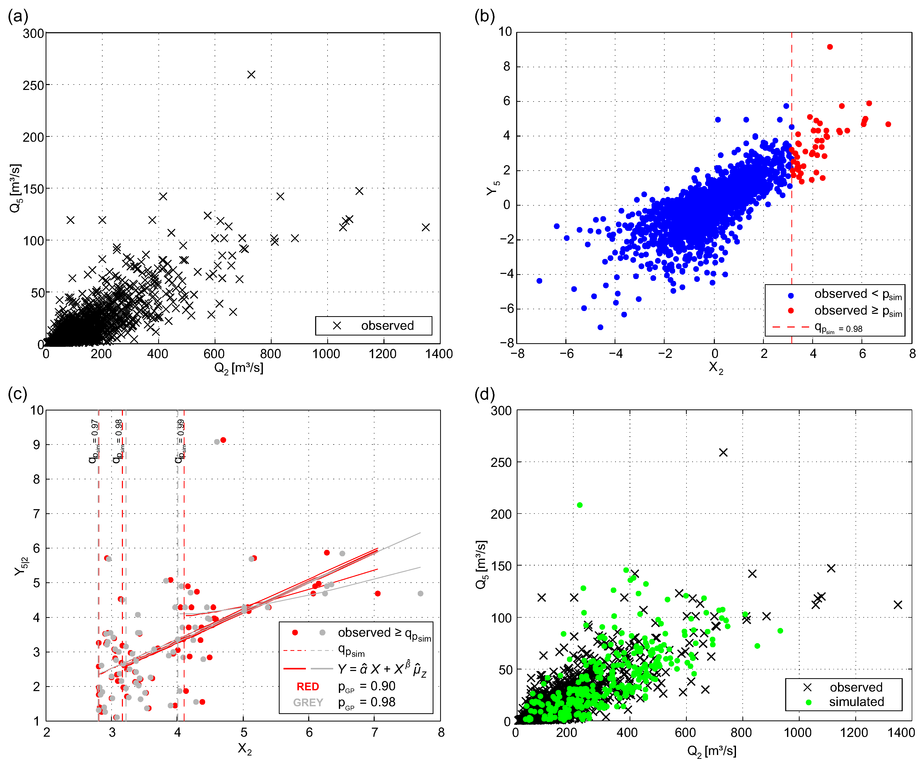
The aim of the simulation is to generate a set of synthetic events S such that at least one of the river flows is extreme—in other words, has an exceedance probability higher than a given . Several steps are involved in fitting the HT model to the data and subsequently to use the fitted model to generate simulated extreme events. These steps are described in some detail below and examples i.e., of sites Kennelbach () and Thal ()) are outlined in Figure 2a–d.
4.3.1. Estimation of Marginal Distribution
As suggested in [20], estimation of the marginal distribution of the runoff variable for is done by using the empirical distribution of the data below some threshold , where is the empirical quantile of the data for some high non-exceedance probability . The Generalized Pareto distribution is fitted to the data above the threshold using a maximum likelihood method. The CDF of this distribution is denoted by . Here, and are the scale and shape parameter of the Generalized Pareto distribution [45]. Hence,
4.3.2. Marginal Transformation
Transformation to Laplace margins is done using the estimated CDF instead of for the marginal transformation using Equation (5). When simulation results are available on a transformed scale, and backwards transformation to real scale is done by
where is the inverse of the empirical distribution for and the inverse of the Generalized Pareto distribution evaluated at for .
4.3.3. Parameter Estimation
To estimate the model parameters and in , we use a quasi maximum likelihood approach [20]. Let be the mean of and its standard deviation, and then and holds. For a pair of transformed observations , where is extreme ( for all t), we set
and estimates of the parameters are given by
The distribution of is not estimated parametrically. Instead, simulation will be based directly on the estimates
This estimation procedure is performed for all possible pairs of data where is extreme.
4.3.4. Simulation of the Conditioning River Flow X
The HT model provides a method to describe the joint conditional distribution of all runoff variables conditional on one being extreme. Before the simulation of the conditional is done, the data to condition on has to be provided, as follows (similar to [28]):
- Number of simulated extreme events per simulation period: The number of extreme events i.e., where at least one site exceeds ) per simulation period (e.g., all-year-, half-year series) is approximated by a negative binominal distribution.
- Selection of conditioning gauge: The set of extreme events S is partitioned to , where is the set of extreme events where gauge i has the highest non-exceedance probability i.e., is the most extreme one). Then, for an event the probability that gauge i is the most extreme if at least one gauge is extreme has to be estimated using given data. The gauge that is selected as conditioning variable X is drawn from a multinomial distribution with these probabilities. Denote the index of the selected gauge by .
- Drawing the conditioning : According to the transformation to standard Laplace margins and since is close to one and hence set , where e is drawn from an exponential distribution with mean one.
4.3.5. Simulation of
Since no parametric model for the distribution of is known, we apply the data based random vector generation method of Taylor and Thompson [46] to the set of vector valued estimates . This method uses m nearest neighbours of a randomly chosen element in , where m is a smoothing parameter. A simulated vector is generated by the following steps:
- Randomly choose one from .
- Find the m nearest neighbours of denoted by and compute the vector of componentwise means of .
- Draw a random sample from a uniform distribution with lower bound and upper bound .
- Deliver .
The smoothing parameter m is chosen and the limits of the uniform distribution from which the weights are drawn from are calculated such that the variance and covariance structure of the data is unchanged, at least approximately.
4.3.6. Simulation of the Dependent Event
When the conditioning value and a sample of are drawn, it is straightforward to compute a sample of the dependent gauges by
If all components of are smaller than , a valid synthetic event is generated. Otherwise, the simulation of and computing has to be repeated.
4.4. HT Model and Seasonal Characteristics of Runoff
The HT model relies on the assumption that river flooding in the winter half-year has the same spatial characteristics as flooding in the summer half-year (cf. Section 3.3 and [22]). The spatial dependence measure is an appropriate tool to investigate whether the spatial characteristics of different series (all-year (), May to October (), and November to April () series) differs significantly. If the assumption does not hold, then the data has to be split into periods that reveal the same spatial characteristics and the HT model has to be applied to both data sets independently.
5. Results and Discussion
Runoff data from selected river gauging stations of the study area Vorarlberg were used (i) for event definition and seasonality analysis, (ii) to conduct a spatial dependence analysis of river flows, (iii) to apply the present multivariate conditional model, and thereby (iv) to generate synthetic (extreme) flood events. The results are based on daily maximum runoff data from 17 representative river gauges in the study area.
As a preliminary remark, note that the number of years simulated with the HT model can be arbitrarily high. This property is essential for the generation of synthetic flood events and for the subsequent evaluation of flood risk. Nevertheless, in this paper, a relatively small simulated data set i.e., year) was used to make the comparison with the observed data (38-year series) reasonable.
5.1. Event Definition and Seasonality of Runoff
Daily maximum runoff data () were analysed using the methods introduced in Section 3.1 in order to identify the most appropriate . Firstly, the results of the measure are summarized in Table 2. For all investigated quantile values p, the probability that an event lasts longer than three days is less than 5%. Secondly, the concentration time (cf. Section 3.1 (ii)) of the selected catchments is displayed in Table 3. Apart from the Rhine catchment at Lustenau (E) (ca. 6000 km2), all sites react relatively quickly ( less than half a day). Thirdly, the flood process typology of annual peaks [36] (cf. Section 2) reveals different relevant flood controls, which hints that the time interval with length of three days is a good compromise. Fourthly, (cf. Section 3.1 (iii)), it should be noted that the presented work is embedded in a flood risk project with a (re)insurance background. In this industry, a time span of 72 h (‘hours clause’) is often used for event definition [47,48]. Based on the three criteria, a time interval with length days was chosen. This time interval guarantees in most cases that consecutive independent flood peaks induced by short rainfall events were considered. On the other hand, days is long enough to ensure that flood peaks in neighboring catchments induced by a single weather pattern will be interpreted as one event. Besides the aspects mentioned above, the idea of the spatial dependence measure can be applied to investigate the temporal dependence in individual series. Therefore, Equation (3) has to be adapted to account for daily maximum data . The dependence measure is then given by [22]. For analysing the temporal dependence of all individual series, was calculated for different p-values. Thus, shows averaged values of the dependence measure over all sites. For a lag of days , , and . For high thresholds (corresponding to or higher), the temporal dependence is less than 5%. Only for low thresholds (corresponding to ) is the temporal independence is not fulfilled; however, this small level of extremeness is not relevant when applying the HT model. Generally, a time interval with a length days ensures temporal independence of events for high thresholds (corresponding to pth quantile). As regularly spaced blocks (i.e., block maxima) were used in this step, it might happen that a block limit falls within a runoff peak at an individual site that can cause the same event to be selected twice. However, as extreme peaks that are relevant in terms of model estimation (above u) are very short (cf. Table 2), a splitting of high peak is extremely rare and thus these cases are negligible.
So far, daily maximum runoff data () were used for data analyses and event definition. The following results are based on maximum runoff in a time interval days i.e., values). Note a quantile value applied to daily data () equals 0.82-year and therefore roughly corresponds to a quantile value applied to values ( 0.91-year).
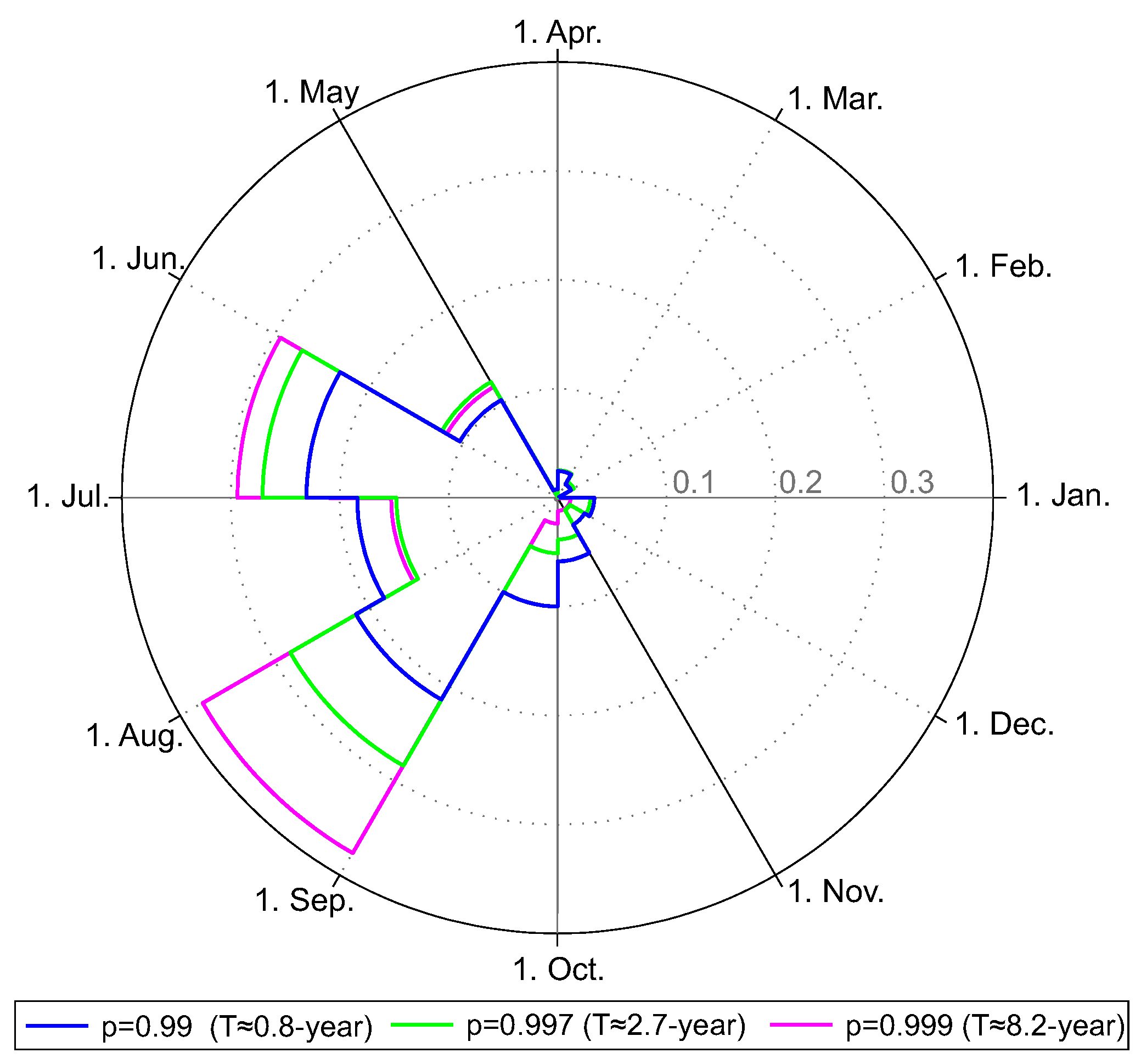
The runoff in the investigated catchment is characterised by strong seasonality, meaning that high flow conditions mainly occur in summer. The mean occurrence date (represented by ) of of all sites is from July to mid of August (Table 3). Following Merz and Blöschl [36], 94% of the catchments experience medium to strong and only 6% weak seasonality, which indicates that in most catchments annual peaks are concentrated around the mean occurrence date. Figure 3 shows monthly frequency of flood peaks above certain threshold values . The results of all sites were combined and plotted in the rose diagram (Figure 3). The figure indicates that flood peaks mainly occur between June and August. Furthermore, Figure 3 shows that from a hydrological perspective a separation of the year into a summer half-year ranging from May to October (), which is dominated by high flow, and in a winter half-year (: November to April), which is characterized by low flow, is reasonable. High flow events above do not usually occur in the winter half-year (events above T ≈ 16-lyear solely occur from May to September, not shown in Figure 3), which reveals that only the summer half-year is relevant for flood risk considerations.
The pronounced seasonality suggests that there is a different spatial characteristic in - and - as well as in the all-year series. Figure 4 shows scatter plots of the spatial dependence measure of 17 sites and for three different p-values for half-year and all-year series. The threshold used in Equation (4) to calculate was derived from the all-year series. To make the results comparable i.e., data from half-year- and all-year series), the pth quantile of half-year series was calculated using where is the pth quantile of all-year series. In Figure 4a, the dependence measure of the all-year series versus the (summer month) is plotted, whereby a strong correlation can be especially observed for high p-values. For and 0.997, the dependence measure for series is systematically lower than for series. Figure 4b shows that the spatial dependence between - and series differs and that the dependence measure for all-year series is systematically higher than for the winter half-year. The distribution-free Wilcoxon test [49] was applied to assess whether and differ significantly. The null hypothesis that the spatial dependence of winter and summer half-year do not differ was rejected for a significance level of 1%. However, the HT model relies on the assumption that flooding in the winter half-year has the same spatial characteristics as flooding in summer half-year [22]. Thus, half-year series were used for further analyses.
5.2. Spatial Dependence in River Flows
The analysis of the spatial dependence of river flows can help to understand the characteristics of widespread flooding. The spatial dependence measures and were calculated for and series, respectively.
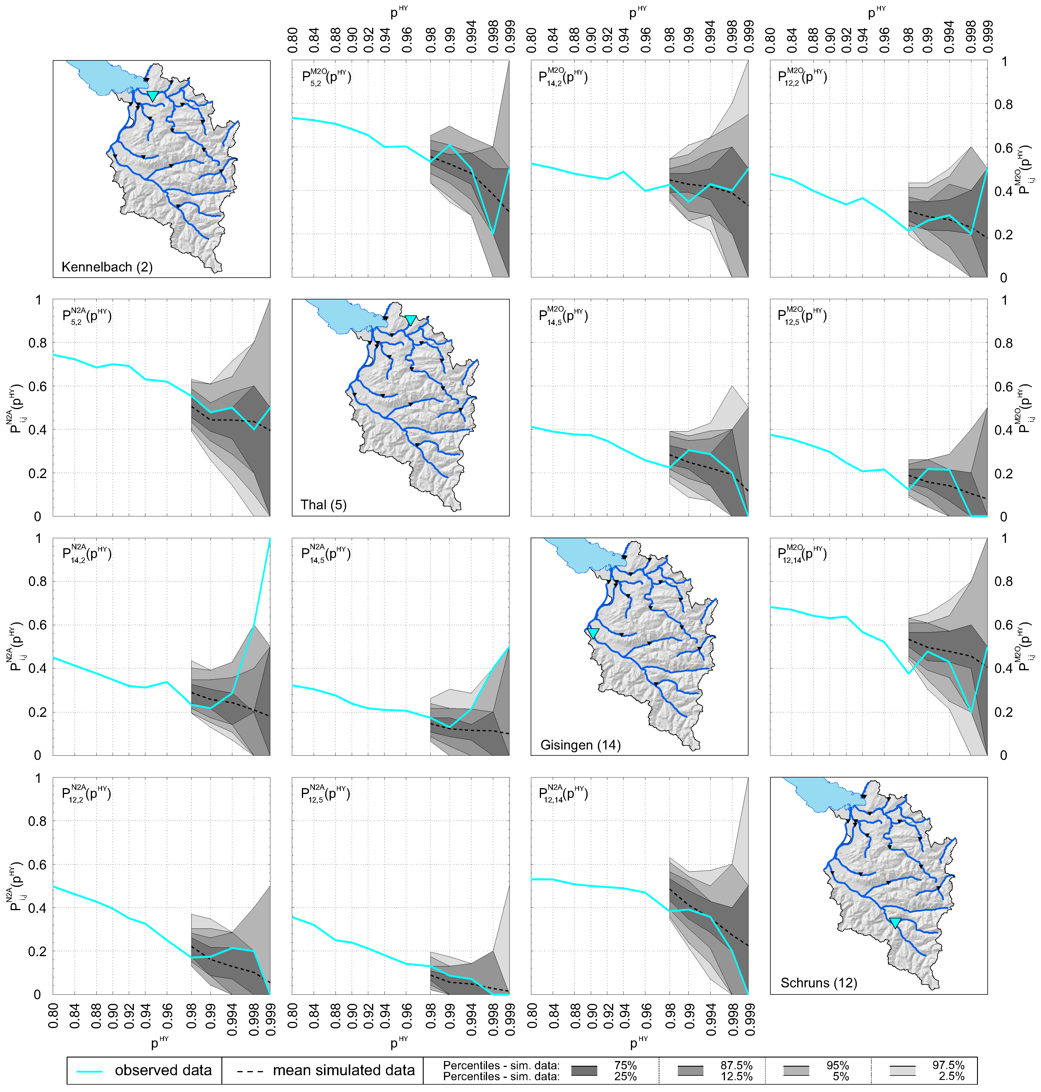
explains the dependence of a pair of variables for a certain threshold , where = 0.4 means that there is a 40% probability of being large i.e., above ) if is above the pth quantile. The spatial dependence measures of four selected stations (Kennelbach, Thal, Gisingen, Schruns) over a range of p are depicted in Figure 5, where (summer half-year) is shown in the upper triangle and (winter half-year) is shown in the lower triangle. of observed data (solid cyan lines) shows the range of dependence between the stations. There is a relatively strong spatial dependence for low p-values between nested catchments where the downward propagation of flood wave plays an important role (e.g., Kennelbach and Thal as well as Gisingen and Schruns), whereas varies markedly for high p-values. The dependence of summer half-years between the stations Kennelbach and Gisingen is fairly equally spread over the entire range of p. These watersheds are relatively large and therefore more vulnerable to long-rainfall events triggered by advective storm systems that affect the entire study area. In Figure 5, the lowest dependence can be found between the stations Thal and Schruns. This is because the watersheds are relatively small and their hydrological characteristics differ significantly [35]. Generally, the spatial dependence between stations in the summer half-year is stronger than in the winter half-year; in 65% of all possible combinations, i.e., 272 cases), is higher than (averaged over p). The most obvious differences between and appear between station Kennelbach and Gisingen as well as Thal and Gisingen, where is high for large p.
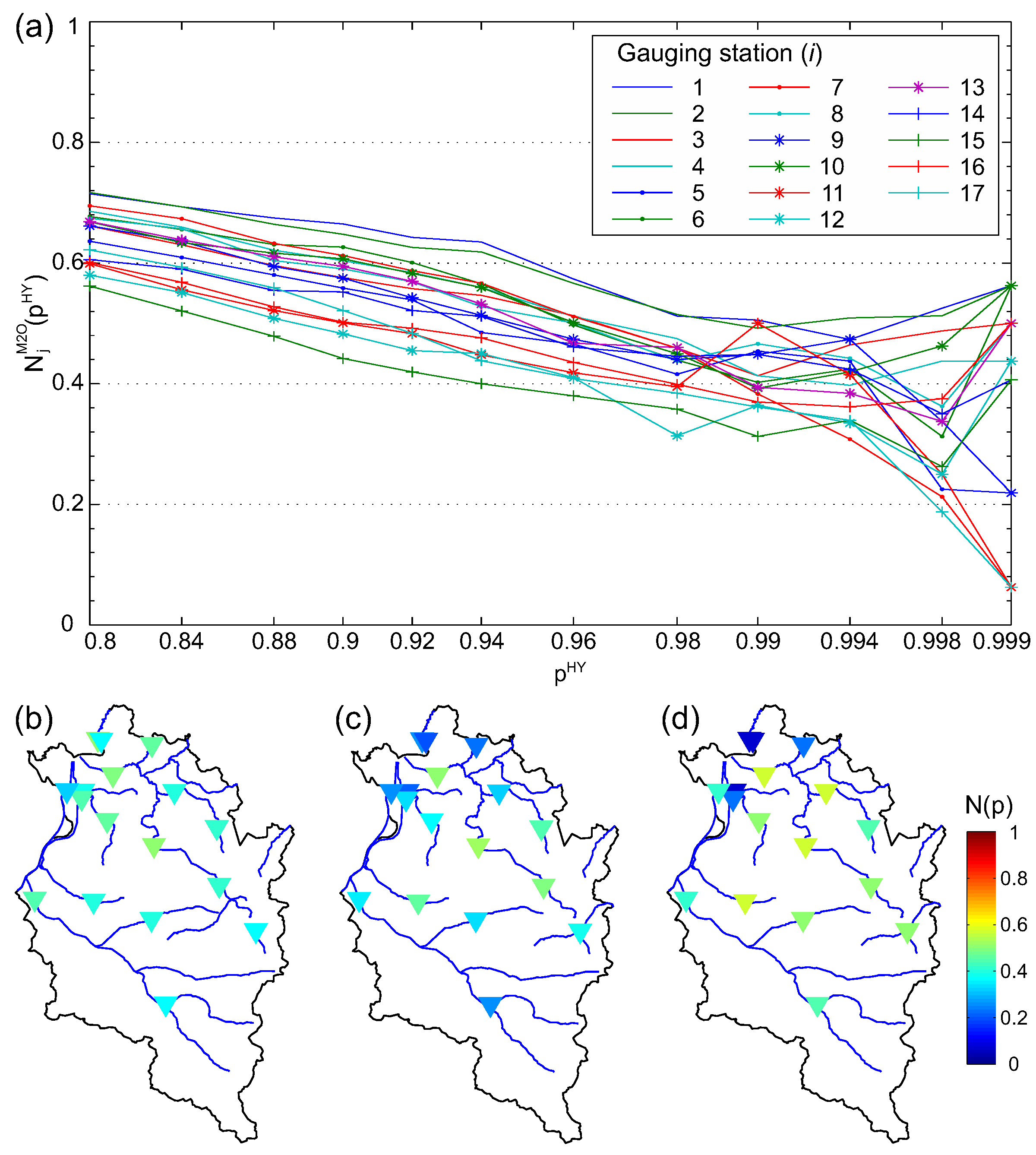
The second spatial dependence measure can be interpreted, as synopsis of over a range of i. In contrast to Keef et al. [22], who investigated the spatial dependence of river flow and precipitation across GB by analysing of stations within a defined radius (30 and 60 km), we analysed the spatial dependence over the entire study area i.e., consideration of all stations). This is reasonable since the entire study area is relatively small and widespread flooding across the study area is relevant for the Province of Vorarlberg.
Figure 6 shows the spatial dependence measure for the summer half-year. Similar to the first dependence measure, a comparison of and reveals that the dependence in summer is higher than in winter i.e., in 77% of possible combinations, is higher than ). Figure 6a illustrates over a range of . Overall, the plot indicates that the estimated dependence between the sites decreases with increasing . In general, the stations located at the same river (nested catchments) show high dependence (e.g., Kennelbach, Mellau, Hopfreben). Data from small headwater catchments and catchments that are situated on the edge of the study area often show low dependence (e.g., Thal, Unterhochsteg, Lochau). In particular, for these stations, increases with higher i.e., fewer data involved in the analysis), because these small catchments seem to be particularly vulnerable to synoptic weather patterns, which in turn are often responsible for the most extreme events in small catchments. Furthermore, the above-mentioned stations with low dependence lie within a radius of 5 km, which indicates that spatial proximity does not guarantee similar behaviour.
As the entire study has ,a distinct flood risk background, spatial dependence of rare events was studied in detail. Therefore, we illustrate for equal to 0.99, 0.998, and 0.999, which correspond to 1.6, 8.2, and 16.4-year in maps of Vorarlberg (Figure 6b–d). The gauges are coloured according to . Figure 6c is particularly suitable for detailed discussion as is based on a reasonable number of events and is high enough to analyse the dependence of severe flood events. Overall, the stations can be divided into three groups according to their spatial dependence: (i) low dependence (stations: Thal, Hoher Steg, Unterhochsteg, Schruns, Lustenau (E), Lochau); (ii) moderate dependence (stations: Lingenau, Enz, Lustenau (H), Garsella, Gisingen, Lech); and (iii) high dependence (stations: Mellau, Kennelbach, Hopfreben, Schönenbach, Laterns). The sites with high dependence are all located in the region Bregenzerwald, which experiences a high amount of annual precipitation.
5.3. Estimation Results and Model Checks
The estimation and simulation procedures outlined in Section 4.3, which were implemented in Matlab (The Mathworks, Natick, MA, USA), were carried out using the data from summer and winter half-year. The interim results of the bivariate case are illustrated in Figure 2 for data of stations Kennelbach () and Thal () for data of . Figure 2a shows the observed data (, ) on a real scale. The same data are depicted in Figure 2b in a transformed scale, whereas the distribution was applied for data above the threshold . Figure 2c illustrates and in a transformed scale above the threshold . This figure includes data where the marginal distribution was applied above the threshold of (red) and above (grey), respectively. Furthermore, the fitted model () was applied for values with an exceedance probability higher than , 0.98, and 0.99. Figure 2c indicates the influence of the choice of the model parameter on the regression model. The red bold line illustrates the fitted model for the selected model parameters and . The corresponding quantile values of an all-year series would be and . Figure 7 shows data and fitted regression models for periods and for exemplarily chosen stations. Thus, the difference of the models for and periods are apparent, which confirms the necessity of using half-year series.
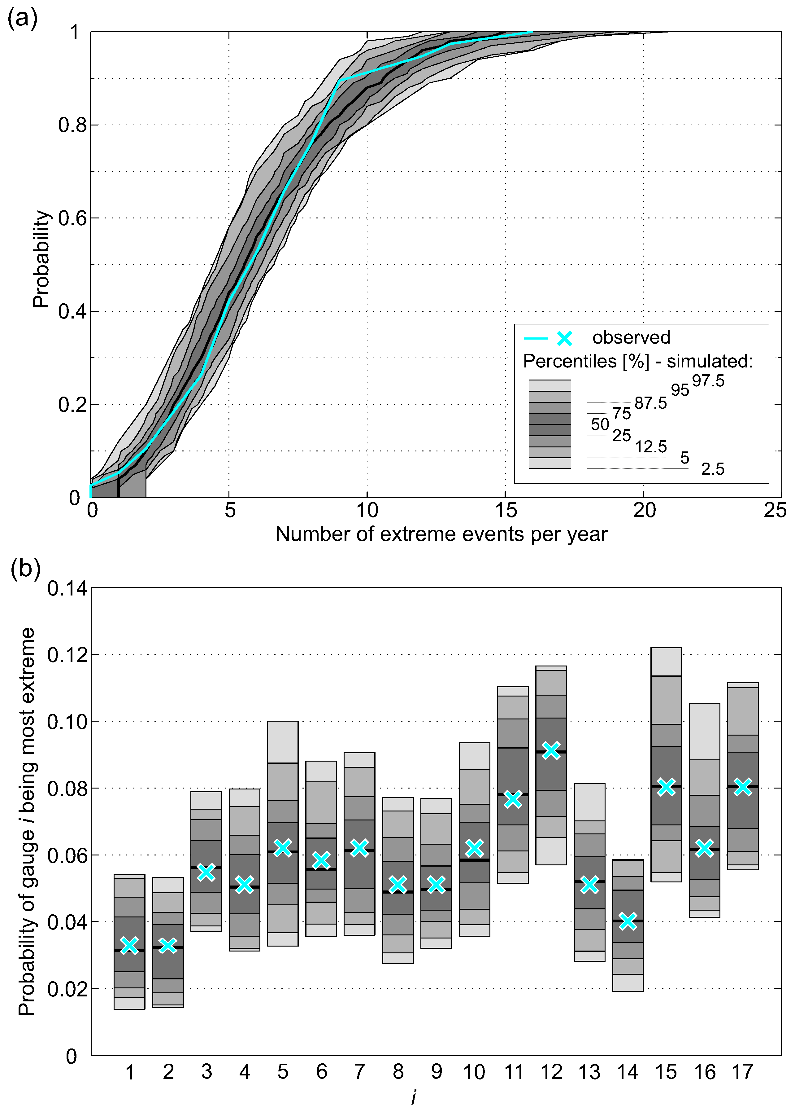
After parameter estimation was done, the simulation procedure starts with the selection of the conditioning river flow. Therefore, the number of extreme events per year was simulated with a negative binomial distribution. Figure 8a shows that the distribution of simulated data is compatible with the empirical distribution of the observed data. The next step was the selection of the conditioning station i i.e., the station with the highest non-exceedance probability. The distribution of the conditioning station is shown in Figure 8b. The cyan crosses represent the probability that one of the 17 gauges is the most extreme based on observed data, and the percentile ranges result from drawing from the multinomial distribution (100 replications). The distribution of the sites with the largest probability of being extreme (Figure 8b) may appear counter-intuitive, as one could expect a uniform distribution. However, the results are in accordance with the findings of Keef et al. [28], who find similar properties of investigated runoff data in GB. Sites that lie on the same river exhibiting high dependences have low probability of being used as conditioning gauge (e.g., sites and 2). Sites with low dependence are expected to have higher probability of being used as conditioning gauges; the four sites with the highest probability ( and 17) are categorized as stations with low spatial dependence (see Section 5.2). After the conditioning site i was selected, its value was drawn.
Before simulating the dependent component (i.e., ), has to be drawn as outlined in Section 4.3.5. The smoothing parameter was chosen with . Finally, a set of spatial dependent extreme events S was simulated. Figure 9d shows a scatterplot (Kennelbach and Thal) in real scale, where green triangles represent simulated events representing years of the simulation period. Note that, although the simulated events can be assigned to a selected time stamp (i.e., year), no continuous time series of river flow was made available.
As no general Goodness-of-Fit test of the HT model exists, several aspects were tested to ensure that the model assumptions were not violated. The first assumption that needs to be checked is that the tails of the marginals are Generalized Pareto distributed. Asymptotically, this assumption is supported by the Pickands–Balkema–de Haan theorem [45]. To assess whether the threshold was high enough, we used the Goodness-of-Fit test for distribution [50]. For thresholds corresponding to , the Generalized Pareto distribution of the tails was never rejected for the 17 investigated river gauges on the 5% significance level; on the 10% significance level, very few rejections appeared. Furthermore, stability of the estimated parameters (see e.g., chap. 4.3.4 in Coles [51]) was checked by visual inspection of parameter estimate plots. This shows that a value of of at least 0.9 is reasonable for all gauges.
Secondly, the assumption of independence of the conditioning variable X and the vector of normalized dependent variables , given that X is above some high threshold, is checked by a series of independence tests for all possible combinations (17 × 16 = 272 combinations) of data with . A statistical test based on Spearman’s was used since no assumptions on the distribution of were made. For , less than 5% of these tests rejected independence on a significance level of 5%. Hence, independence can be considered to hold for values of at least .
The third assumption that the distribution G of is non-degenerated with no mass at is of theoretical interest and automatically fulfilled when G is inferred from data.
A key aspect of all model applications is the compatibility of observed and simulated data. This was checked by comparing several components such as scatterplots of selected gauges, the spatial dependence measures and , and the medians of yearly maximum runoff of the half-year series derived from observed and simulated data. These model checks were used to determine the most suitable model parameters to be and . In the context of model checks, it is important to emphasize that the HT model is valid above a threshold . This implies that a comprehensive set of simulated data was only available for high runoff values. As a consequence, the comparison of observed and simulated data has to be done on the basis of relative ‘extreme’ values.
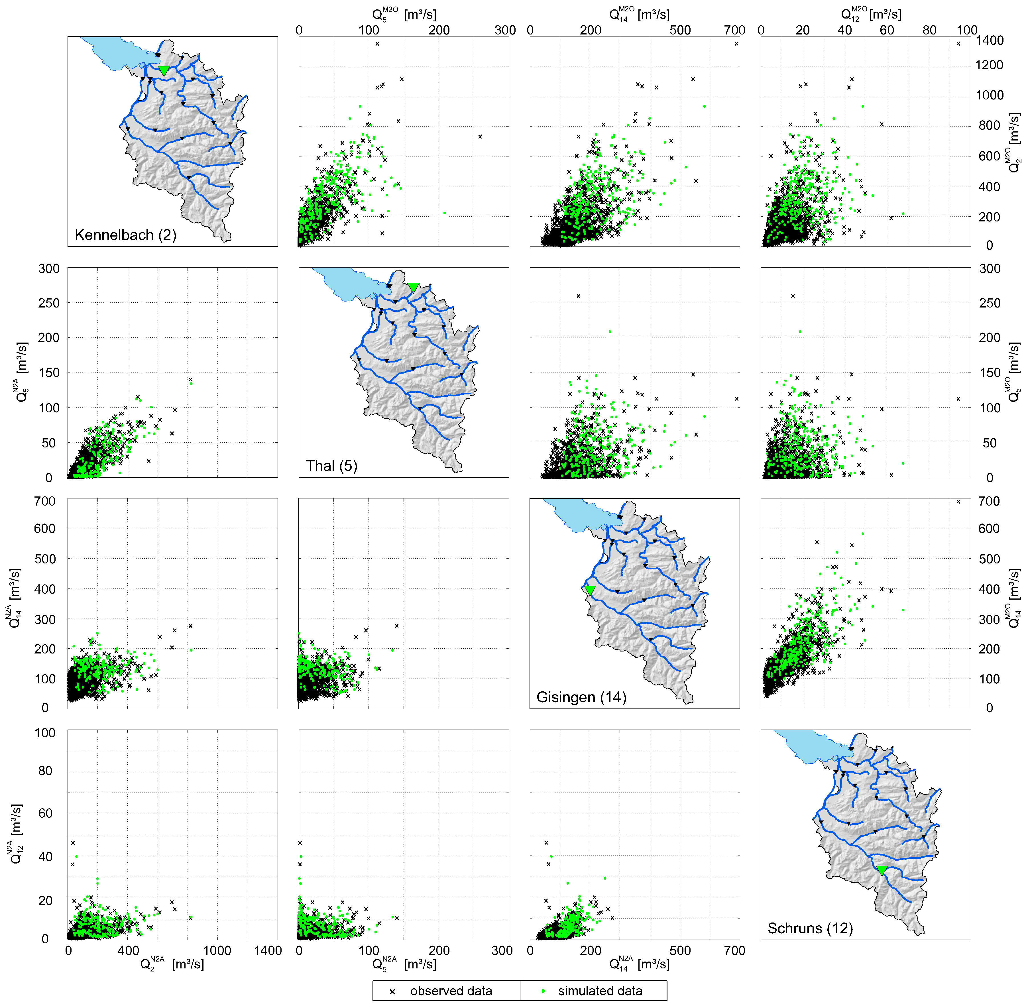
Figure 9 illustrates scatterplots of four representative gauges (Kennelbach, Thal, Gisingen, Schruns) of observed and simulated data (simulation period of 38 years). A visual check shows the range of dependence in the data and indicates that the HT model is flexible enough to reproduce the structure of the data. When the correlation between observed data of two stations is strong, simulated data also reveal strong correlations (e.g., Kennelbach and Gisingen). On the other hand, simulated data are almost arbitrarily distributed when observed data show hardly any correlation (e.g., Thal and Schruns). Figure 9 also illustrates the difference between runoff data of (upper triangle) and (lower triangle). The runoff intensity of the former is considerably higher than the runoff in , which again indicates that a separation of the data into winter and summer half-year is necessary.
Furthermore, the spatial dependence measure of observed and simulated data was compared and depicted in Figure 5. Because of the validity of the HT model above a certain threshold u i.e., ), of simulated data is illustrated for , 0.99, 0.994, 0.998, and 0.999. As illustrated in Figure 5, the dependence measure of observed and simulated data is in the same range. Table 4 shows the systematic comparison for all possible combinations i.e., 272 combinations). (column 3) means that 95% of the observed lies within the specified range (5–95% of simulated data). The results for are slightly higher and show that the model is even better suited to reproduce the spatial dependence of river flow for the winter half-year than for the summer half-year. The systematic analysis of the spatial dependence measure (Table 4) confirms the accordance of simulated and observed data.
The most important model check is probably a systematic comparison of observed and simulated runoff series of each station. Therefore, the use of yearly maximum runoff () of the half-year series seems to be appropriate because this type of series contains only relatively high values. Consequently, of observed data ( and ) and simulated data ( and ) were derived and the medians of each series were compared (Figure 10). Instead of runoff (m3 s−1), the use of specific discharge q (l s−1 km−2) allows for easy comparisons of stations with different catchment size. For the comparison of simulated and observed data, 100 replications with a simulation period of 38 years were generated and percentile ranges were depicted for all stations (Figure 10). The required number of replications has been determined by applying a procedure to obtain a specified precision of confidence intervals [52]. For 100 replications, the 90% confidence interval of the medians of has a relative length of less than 5% for all 17 sites. Figure 10 indicates that observed and simulated values are in accordance for most sites. The systematic comparison of the maximum runoff (cf. the last two lines of Table 4) shows that the HT model is able to reproduce the runoff adequately and that the selected parameters are appropriate.
5.4. Simulated Extreme Events
The main output of the HT model is a set of spatially distributed flood events S on defined locations i.e., river gauges). As the runoff intensity of the summer half-year (see also Figure 3) is considerably higher than the intensity of the winter half-year, only events from were considered here. In a first step, the information about the intensity of these events was made available in real scale i.e., m3 s−1) for each individual event and every station. To enable a further usage of the synthetic events, it was necessary to define the so-called level of extremeness [21] for all events and every single station on a probability scale. This probability scale corresponds to the concept of return period of hydraulic loads.
The link between physical scale (m3 s−1) and ‘return period’ scale, which corresponds to ‘probability’ scale, was constructed by applying the Generalized Extreme Value () distribution. The method of L-moments [53] was used to fit the distribution to the of observed data of all stations and a Goodness-of-Fit test was carried out to check the suitability of this distribution. The distribution was never rejected at a 5% significance level for the 17 investigated stations. Furthermore, previous studies pointed out that the distribution is an appropriate distribution function within the region [35,54,55].
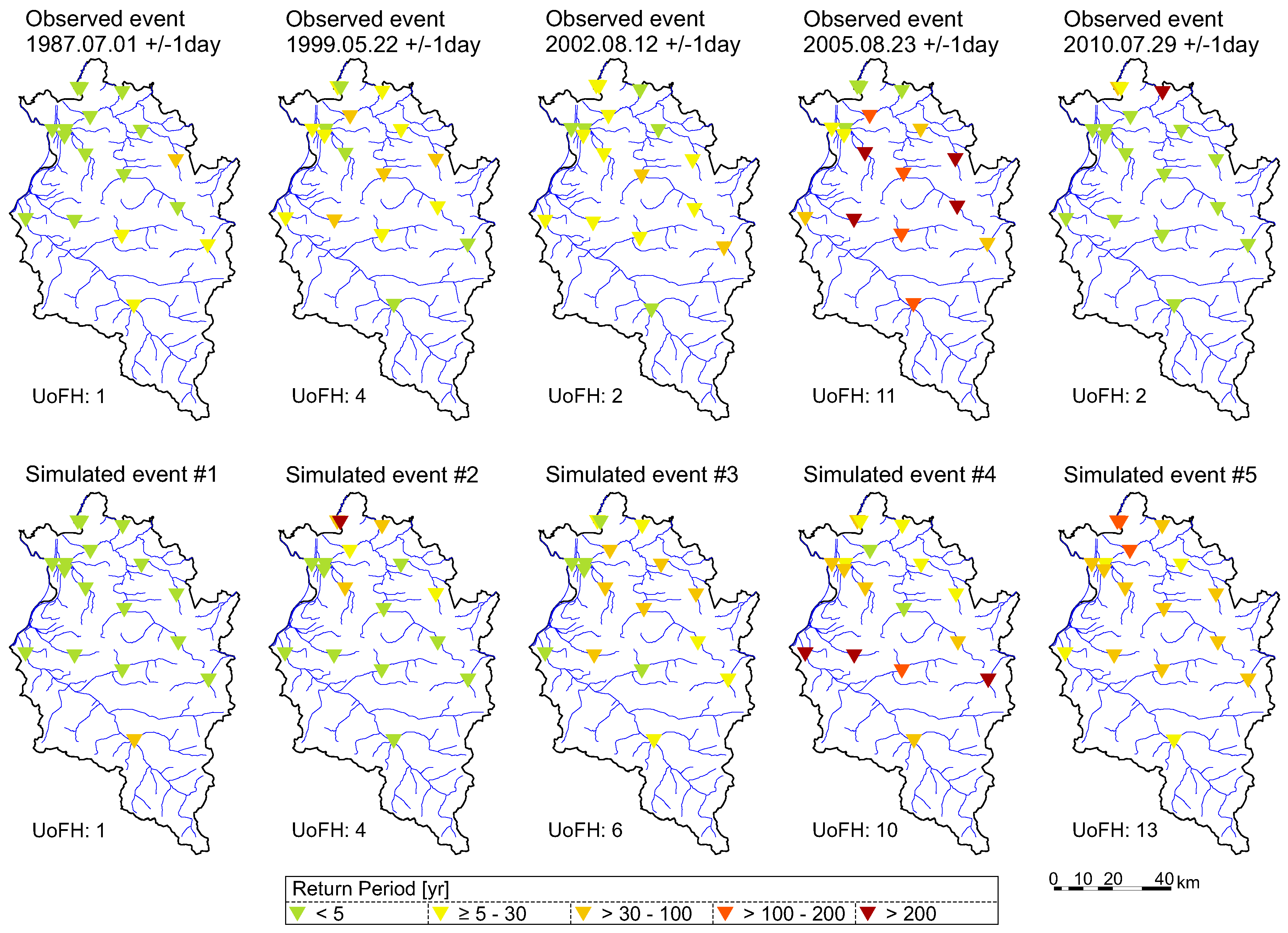
Figure 11 shows five observed and five simulated flood events where the color of the triangles represents the return period that occurs on each station. The synthetic events reveal a reasonable spatial dependence structure that can also be found in observed flood events. For further analyses, only severe flood events are of interest, where one or multiple stations exceed a T ≥ 30-year. The severity of the illustrated flood events was categorized by the measure unit of flood hazard (see Section 3.2), which is indicated on the bottom of each map. For comparison, following the categorization of the UoFH, nine events were identified in the period 1976–2013, and the most severe observed flood event (August 2005) was categorized as a 12 UoFH-event i.e., the runoff was equal to or exceeded a threshold that corresponded to a return period 30-year at 12 river gauges).
6. Conclusions
In this paper, we have demonstrated that the HT model [20] can be successfully applied in a complex mountain topography with high runoff seasonality. However, before applying the conditional dependence model, a priori data review and preparation is essential in order to avoid violation of the model assumptions. A thorough data analysis of daily maximum data of 17 river gauging stations in the study area Vorarlberg shows that a time interval of three days is most suitable for event definition. Because of the pronounced seasonality of runoff and the different spatial characteristics in the half-year series, a separation of the all-year series was necessary. Thus, the conditional model was driven with time series from and .
The spatial characteristics of widespread and often spatially heterogeneous flood events were analysed. Therefore, the spatial dependence measures and were calculated in order to improve the understanding of the spatial characteristics of widespread river flood events. River gauging stations were identified where high runoff likely occurs simultaneously with other stations and, on the other hand, stations were found that show hardly any spatial dependence with other stations.
By applying the HT model, a set of synthetic flood events were generated. These extreme events represent a large range of possible flooding situations as they could occur in the investigated region. The set of synthetic flood events serves as a surrogate for probabilistic flood risk analysis. The severity of individual flood events was categorized by a simplistic hydrological proxy (units of flood hazard). The present modeling procedure can be applied wherever a dense network of river gauging measurements exist that capture the spatial characteristics of flood events in a specific region.
The analysis that is shown here does not include considerations about the potential adverse consequences of flooding. However, for a comprehensive analysis of flood risk, the following aspects are indispensable. Besides the generation of synthetic flood events, the adverse consequences of flooding have to be quantified (e.g., the monetary damage of buildings) and the overall flood risk within a region has to be assessed. Schneeberger et al. [33] introduces a probabilistic framework for risk analysis, which takes into account all relevant aspects and requires a set of spatially distributed flood events.
Acknowledgments
This work results from the research project InsuRE funded by the Austrian Research Promotion Agency (FFG) within the scope of the programme COMET, the Tyrolean Insurance Company (Tiroler Versicherung), and the Vorarlberger Insurance Company (Vorarlberger Landesversicherung). We would like to thank all the institutions that provided data, particularly the Hydrographic Service of Vorarlberg. K.S. acknowledges the financial support provided through the scholarship Nachwuchsförderung der Universität Innsbruck. We are grateful to all reviewers for the insightful and helpful comments to previous versions of the manuscript.
Author Contributions
K.S. and T.S. conceived and designed the experiments; K.S. and T.S. analyzed the data; T.S. and K.S. developed and implemented the applied method; K.S. and T.S. wrote the paper.
Conflicts of Interest
The authors declare no conflict of interest.
Abbreviations
The following abbreviations are used in this manuscript:
| HT model | Multivariate semi-parametric conditional model introduced by Heffernan and Tawn (2004) [20] |
| T | Return period in year |
| Annual maximum series | |
| AMS derived from daily mean data | |
| AMS derived from daily maximum data | |
| UoFH | Unit of flood hazard |
| All-year (series) | |
| General extreme value (distribution) | |
| Yearly maximum runoff (of half-year series) | |
| May to October (series) | |
| November to April (series) |
References
- National Research Council (NRC). Flood Risk Management and the American River Basin: An Evaluation; National Academies Press: Washington, DC, USA, 1995. [Google Scholar]
- European Union. On the assessment and management of flood risks: Directive 2007/60/EC of the European Parliament and the Council. Off. J. Eur. Community 2007, 288, 27–34. [Google Scholar]
- FLOODsite. Lanugauge of Risk: Project Definitions, 2nd ed.; HR Wallingford: Wallingford, UK, 2009. [Google Scholar]
- Uhlemann, S.; Thieken, A.H.; Merz, B. A consistent set of trans-basin floods in Germany between 1952–2002. Hydrol. Earth Syst. Sci. 2010, 14, 1277–1295. [Google Scholar] [CrossRef]
- Leonard, M.; Westra, S.; Phatak, A.; Lambert, M.; van den Hurk, B.; McInnes, K.; Risbey, J.; Schuster, S.; Jakob, D.; Stafford-Smith, M. A compound event framework for understanding extreme impacts. Wiley Interdiscip. Rev. Clim. Chang. 2014, 5, 113–128. [Google Scholar] [CrossRef]
- Thieken, A.H.; Apel, H.; Merz, B. Assessing the probability of large-scale flood loss events: A case study for the river Rhine, Germany. J. Flood Risk Manag. 2015, 8, 247–262. [Google Scholar] [CrossRef]
- Falter, D.; Dung, N.V.; Vorogushyn, S.; Schröter, K.; Hundecha, Y.; Kreibich, H.; Apel, H.; Theisselmann, F.; Merz, B. Continuous, large-scale simulation model for flood risk assessments: Proof-of-concept. J. Flood Risk Manag. 2016, 9, 9–21. [Google Scholar] [CrossRef]
- Jongman, B.; Hochrainer-Stigler, S.; Feyen, L.; Aerts, J.C.J.H.; Mechler, R.; Botzen, W.J.W.; Bouwer, L.M.; Pflug, G.; Rojas, R.; Ward, P.J. Increasing stress on disaster-risk finance due to large floods. Nat. Clim. Chang. 2014, 4, 264–268. [Google Scholar] [CrossRef]
- Falter, D.; Schröter, K.; Nguyen, V.D.; Vorogushyn, S.; Kreibich, H.; Hundecha, Y.; Apel, H.; Merz, B. Spatially coherent flood risk assessment based on long-term continuous simulation with a coupled model chain. J. Hydrol. 2015, 524, 182–193. [Google Scholar] [CrossRef]
- Renard, B.; Lang, M. Use of a Gaussian copula for multivariate extreme value analysis: Some case studies in hydrology. Adv. Water Res. 2007, 30, 897–912. [Google Scholar] [CrossRef]
- Genest, C.; Favre, A.C.; Béliveau, J.; Jacques, C. Metaelliptical copulas and their use in frequency analysis of multivariate hydrological data. Water Resour. Res. 2007, 43, 1–12. [Google Scholar] [CrossRef]
- Schölzel, C.; Friederichs, P. Multivariate non-normally distributed random variables in climate research— Introduction to the copula approach. Nonlinear Process. Geophys. 2008, 15, 761–772. [Google Scholar] [CrossRef]
- Klein, B.; Pahlow, M.; Hundecha, Y.; Schumann, A. Probability Analysis of Hydrological Loads for the Design of Flood Control Systems Using Copulas. J. Hydrol. Eng. 2010, 15, 360–369. [Google Scholar] [CrossRef]
- Kilgore, R.; Thompson, D.B.; Ford, D.T. Estimating the Joint Probability of Coincident Flows at Stream Confluences. In World Environmental and Water Resources Congress 2011; Beighley, R.E., Killgore, M.W., Eds.; American Society of Civil Engineers: Reston, VA, USA, 2011. [Google Scholar]
- Chen, L.; Singh, V.P.; Shenglian, G.; Hao, Z.; Li, T. Flood Coincidence Risk Analysis Using Multivariate Copula Functions. J. Hydrol. Eng. 2012, 17, 742–755. [Google Scholar] [CrossRef]
- Requena, A.I.; Mediero, L.; Garrote, L. A bivariate return period based on copulas for hydrologic dam design: accounting for reservoir routing in risk estimation. Hydrol. Earth Syst. Sci. 2013, 17, 3023–3038. [Google Scholar] [CrossRef]
- Sraj, M.; Bezak, N.; Brilly, M. Bivariate flood frequency analysis using the copula function: A case study of the Litija station on the Sava River. Hydrol. Process. 2015, 29, 225–238. [Google Scholar] [CrossRef]
- Durocher, M.; Chebana, F.; Ouarda, T.B. On the prediction of extreme flood quantiles at ungauged locations with spatial copula. J. Hydrol. 2016, 533, 523–532. [Google Scholar] [CrossRef]
- Requena, A.I.; Chebana, F.; Mediero, L. A complete procedure for multivariate index-flood model application. J. Hydrol. 2016, 535, 559–580. [Google Scholar] [CrossRef]
- Heffernan, J.E.; Tawn, J.A. A conditional approach for multivariate extreme values (with discussion). J. R. Stat. Soc. B 2004, 66, 497–546. [Google Scholar] [CrossRef]
- Lamb, R.; Keef, C.; Tawn, J.A.; Laeger, S.; Meadowcroft, I.; Surendran, S.; Dunning, P.; Batstone, C. A new method to assess the risk of local and widespread flooding on rivers and coasts. J. Flood Risk Manag. 2010, 3, 323–336. [Google Scholar] [CrossRef]
- Keef, C.; Svensson, C.; Tawn, J.A. Spatial dependence in extreme river flows and precipitation for Great Britain. J. Hydrol. 2009, 378, 240–252. [Google Scholar] [Green Version]
- Jonathan, P.; Flynn, J.; Ewans, K. Joint modelling of wave spectral parameters for extreme sea states. Ocean Eng. 2010, 37, 1070–1080. [Google Scholar] [CrossRef]
- Ewans, K.; Jonathan, P. Evaluating environmental joint extremes for the offshore industry using the conditional extremes model. J. Mar. Syst. 2014, 130, 124–130. [Google Scholar] [CrossRef]
- Gouldby, B.; Mendez, F.; Guanche, Y.; Rueda, A.; Minguez, R. A methodology for deriving extreme nearshore sea conditions for structural design and flood risk analysis. Coast. Eng. 2014, 88, 15–26. [Google Scholar] [CrossRef]
- Keef, C.; Tawn, J.A.; Svensson, C. Spatial risk assessment for extreme river flows. Appl. Stat. 2009, 58, 601–618. [Google Scholar] [CrossRef]
- Mendes, B.V.D.M.; Pericchi, L.R. Assessing conditional extremal risk of flooding in Puerto Rico. Stoch. Environ. Res. Risk Assess. 2009, 23, 399–410. [Google Scholar] [CrossRef]
- Keef, C.; Tawn, J.A.; Lamb, R. Estimating the probability of widespread flood events. Environmetrics 2013, 24, 13–21. [Google Scholar] [CrossRef]
- Neal, J.; Keef, C.; Bates, P.D.; Beven, K.; Leedal, D. Probabilistic flood risk mapping including spatial dependence. Hydrol. Process. 2013, 27, 1349–1363. [Google Scholar] [CrossRef]
- Wyncoll, D.; Gouldby, B. Integrating a multivariate extreme value method within a system flood risk analysis model. J. Flood Risk Manag. 2015, 8, 145–160. [Google Scholar] [CrossRef]
- Speight, L.; Hall, J.; Kilsby, C. A multi-scale framework for flood risk analysis at spatially distributed locations. J. Flood Risk Manag. 2017, 10, 124–137. [Google Scholar] [CrossRef]
- Habersack, H.; Krapesch, G. Hochwasser 2005—Ereignisdokumentation: Der Bundeswasserbauverwaltung, des Forsttechnischen Dienstes für Wildbach- und Lawinenverbauung und des Hydrographischen Dienstes; Bundesministerium für Land- und Forstwirtschaft, Umwelt- und Wasserwirtschaft: Vienna, Austria, 2006. [Google Scholar]
- Schneeberger, K.; Huttenlau, M.; Winter, B.; Steinberger, T.; Achleitner, S.; Stötter, J. A probabilistic framework for risk analysis of widespread flood events: A proof-of-concept study. Risk Anal. 2017. [Google Scholar] [CrossRef] [PubMed]
- Gaál, L.; Szolgay, J.; Kohnová, S.; Parajka, J.; Merz, R.; Viglione, A.; Blöschl, G. Flood timescales: Understanding the interplay of climate and catchment processes through comparative hydrology. Water Resour. Res. 2012, 48. [Google Scholar] [CrossRef]
- Schneeberger, K.; Huttenlau, M.; Stötter, J. A Seasonality Analysis of Flood Peaks as Basis for Flood Risk Analyses in two Alpine Regions. In Proceedings of the 3rd STAHY International Workshop on Statistical Methods for Hydrology and Water Resources Management, Tunis, Tunisia, 1–2 October 2012. [Google Scholar]
- Merz, R.; Blöschl, G. A process typology of regional floods. Water Resour. Res. 2003, 39, 1340–1359. [Google Scholar] [CrossRef]
- Hawkes, P.J.; Gonzalez-Marco, D.; Sánchez-Arcilla, A.; Prinos, P. Best practice for the estimation of extremes: A review. J. Hydraul. Res. 2008, 46, 324–332. [Google Scholar] [CrossRef]
- Grimaldi, S.; Petroselli, A.; Tauro, F.; Porfiri, M. Time of concentration: a paradox in modern hydrology. Hydrol. Sci. J. 2012, 57, 217–228. [Google Scholar] [CrossRef]
- Keef, C.; Lamb, R.; Tawn, J.A.; Laeger, S. A multivariate model for the broad scale spatial assessment of flood risk. In Proceedings of the BHS Third International Symposium, Managing Consequences of a Changing Global Environment, Newcastle, UK, 19–23 July 2010. [Google Scholar]
- Mardia, K.V.; Jupp, P.E. Statistics of Directional Data, 2nd ed.; Wiley Series in Probability and Statistics; Wiley: New York, NY, USA, 1999. [Google Scholar]
- Schneeberger, K.; Dobler, C.; Huttenlau, M.; Stötter, J. Assessing potential climate change impacts on the seasonality of runoff in an Alpine watershed. J. Water Clim. Chang. 2015. [Google Scholar] [CrossRef]
- Burn, D.H. Catchment similarity for regional flood frequency analysis using seasonality measures. J. Hydrol. 1997, 202, 212–230. [Google Scholar] [CrossRef]
- De Michele, C.; Rosso, R. A multi-level approach to flood frequency regionalisation. Hydrol. Earth Syst. Sci. 2002, 6, 185–194. [Google Scholar] [CrossRef]
- Keef, C.; Papastathopoulos, I.; Tawn, J.A. Estimation of the conditional distribution of a multivariate variable given that one of its components is large: Additional constraints for the Heffernan and Tawn model. J. Multivar. Anal. 2013, 115, 396–404. [Google Scholar] [CrossRef]
- Embrechts, P.; Klüppelberg, C.; Mikosch, T. Modelling Extremal Events: For Insurance and Finance; Stochastic Modelling and Applied Probability; Springer: Berlin/Heidelberg, Germany, 1997; Volume 33. [Google Scholar]
- Taylor, M.S.; Thompson, J.R. A data based algorithm for the generation of random vectors. Comput. Stat. Data Anal. 1986, 4, 93–101. [Google Scholar] [CrossRef]
- Holub, M.; Gruber, H.; Fuchs, S. Risks from natural hazards in the insurance business. In Studienreise 2010—Risiko im Bereich Schutz vor Naturgefahren; Skolaut, C., Ed.; Wildbach- und Lawinenverbau; Verein der Diplomingenieure der Wildbach-und Lawinenverbauung Österreichs: Villach, Austria, 2011; Volume 167. [Google Scholar]
- Serinaldi, F.; Kilsby, C.G. A Blueprint for Full Collective Flood Risk Estimation: Demonstration for European River Flooding. Risk Anal. 2017, 37, 1958–1976. [Google Scholar] [CrossRef] [PubMed]
- Bortz, J.; Schuster, C. Statistik für Human- und Sozialwissenschaftler, 7th ed.; Springer-Lehrbuch; Springer: Berlin, Germany, 2010. [Google Scholar]
- Choulakian, V.; Stephens, M.A. Goodness-of-Fit Tests for the Generalized Pareto Distribution. Technometrics 2001, 43, 478–484. [Google Scholar] [CrossRef]
- Coles, S. An Introduction to Statistical Modeling of Extreme Values; Springer Series in Statistics; Springer: London, UK; New York, NY, USA, 2001. [Google Scholar]
- Law, A.; Kelton, W. Simulation Modelling and Analysis; McGraw-Hill Series in Industrial Engineering and Management Science; McGraw-Hill: New York, NY, USA, 2000. [Google Scholar]
- Hosking, J.R.M.; Wallis, J.R. Regional Frequency Analysis: An Approach Based on L-Moments; Cambridge University Press: Cambridge, UK; New York, NY, USA, 1997. [Google Scholar]
- Merz, R.; Blöschl, G. Flood frequency regionalisation—Spatial proximity vs. catchment attributes. J. Hydrol. 2005, 302, 283–306. [Google Scholar] [CrossRef]
- Petrow, T.; Merz, B.; Lindenschmidt, K.E.; Thieken, A.H. Aspects of seasonality and flood generating circulation patterns in a mountainous catchment in south-eastern Germany. Hydrol. Earth Syst. Sci. 2007, 11, 1455–1468. [Google Scholar] [CrossRef]
Figure 1.
Study area Vorarlberg and the location of river runoff gauges.
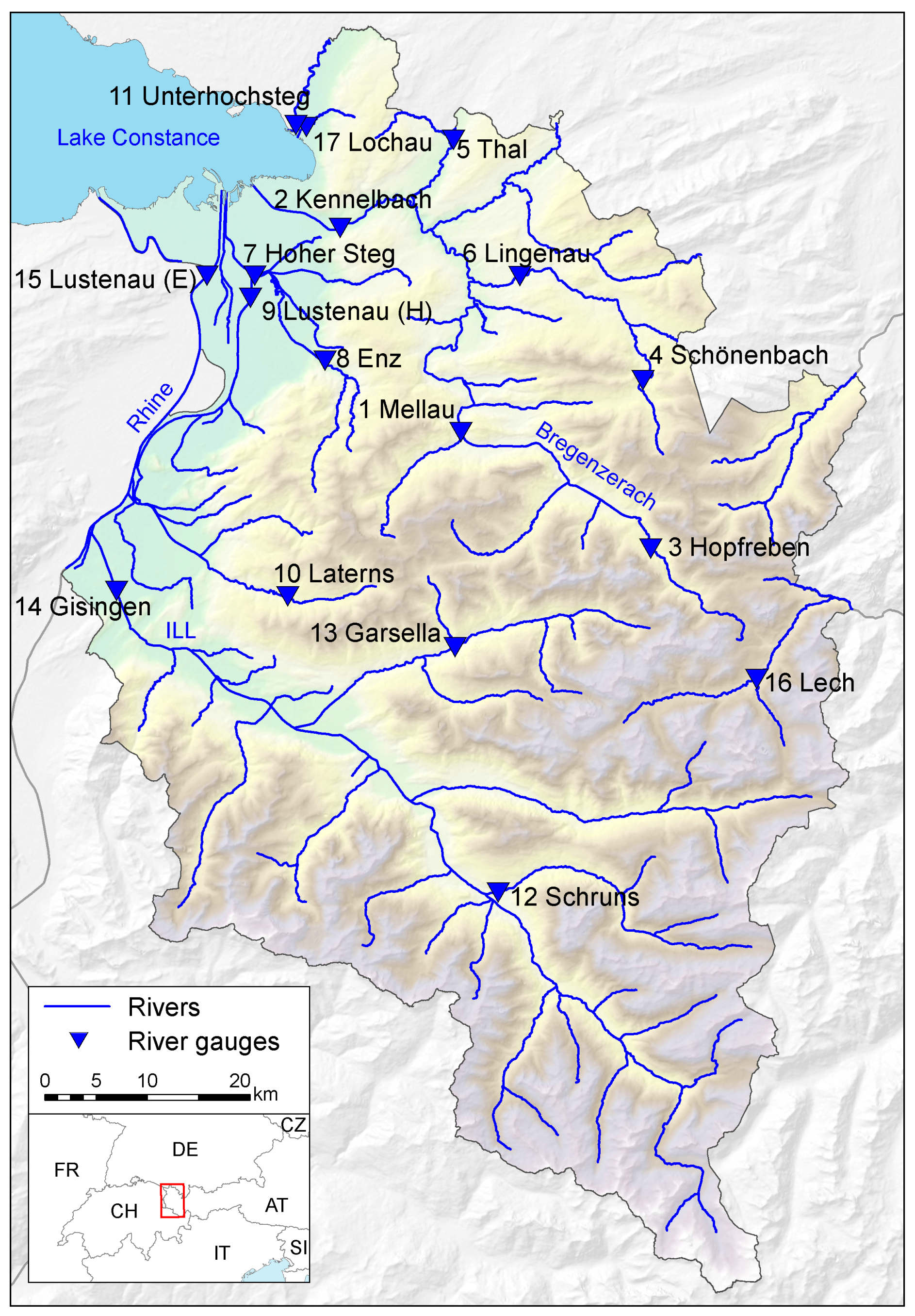
Figure 2.
Scatterplot of observed and simulated data from half-year series (May to October) of gauges Kennelbach () and Thal (), statistical model, and model thresholds: (a) observed data in real scale; (b) observed data (threshold for marginal distribution ) in transformed scale, incl. ; (c) observed data in transformed scale (values above ), incl. fitted model (red color indicates that the distribution was applied above the threshold ; grey color indicates ); and (d) observed and simulated data ( year) on a real scale.

Figure 3.
Rose diagram of runoff (for all ) above threshold values ().

Figure 4.
Comparison of spatial dependence measure derived from all-year and half-year series: (a) versus and (b) versus .
Figure 4.
Comparison of spatial dependence measure derived from all-year and half-year series: (a) versus and (b) versus .
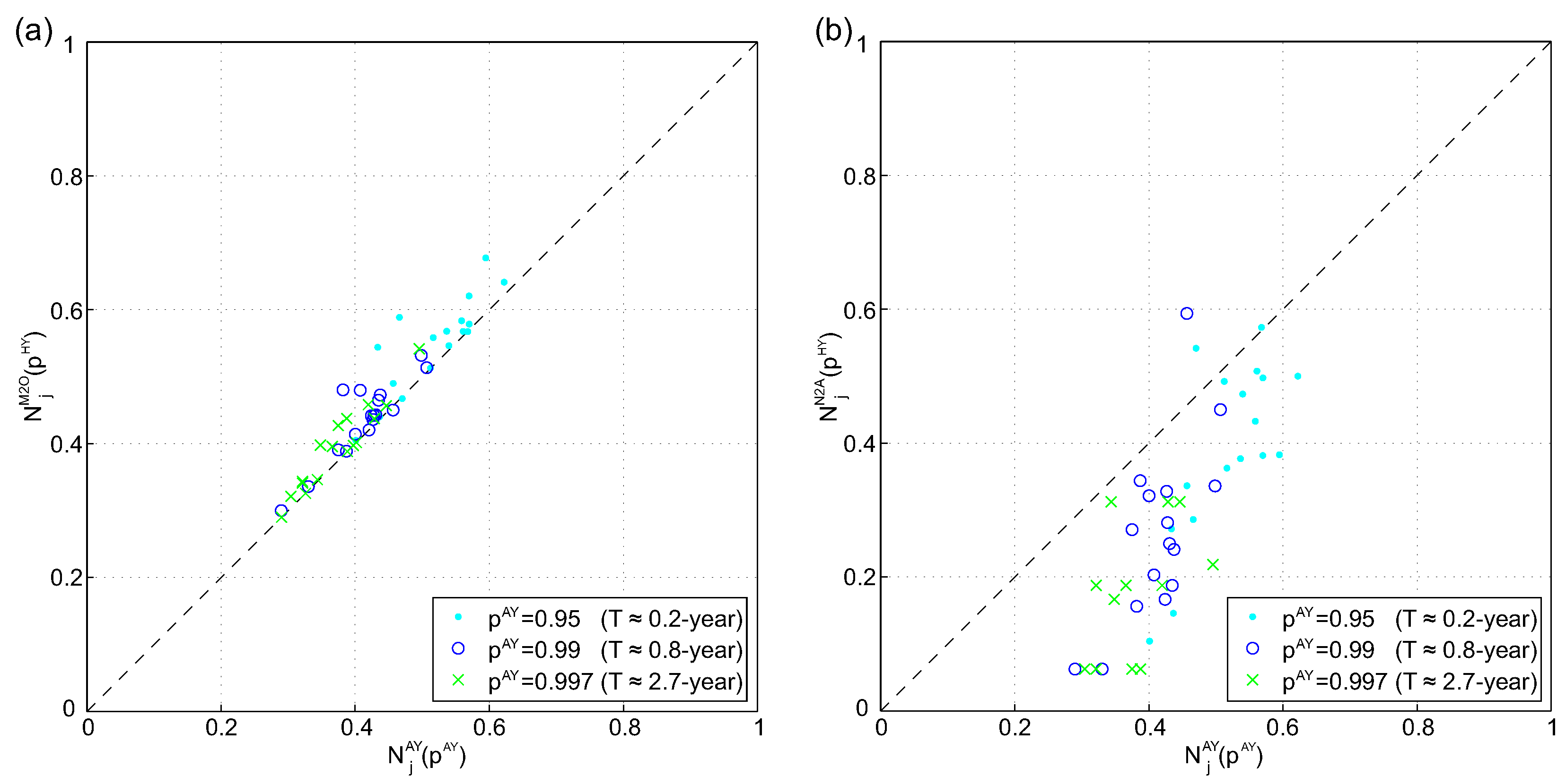
Figure 5.
Spatial dependence measure against non-exceedance probability of observed and simulated (100 × 38 year) runoff data of station Kennelbach (), Thal (), Gisingen (), and Schruns (). Upper triangle: . Lower triangle: .
Figure 5.
Spatial dependence measure against non-exceedance probability of observed and simulated (100 × 38 year) runoff data of station Kennelbach (), Thal (), Gisingen (), and Schruns (). Upper triangle: . Lower triangle: .

Figure 6.
(a) spatial dependence measure against non-exceedance probability ; (b–d) dependence measure depicted in a map of Vorarlberg with colored gauging stations representing , corresponding to (b) ( 1.6-year); (c) ( 8.2-year), and (d) ( 16.4-year).
Figure 6.
(a) spatial dependence measure against non-exceedance probability ; (b–d) dependence measure depicted in a map of Vorarlberg with colored gauging stations representing , corresponding to (b) ( 1.6-year); (c) ( 8.2-year), and (d) ( 16.4-year).

Figure 7.
Observed data from and in transformed scale (values above ) incl. fitted model conditioned on (Gisingen) and dependend: (a) (Kennelbach); (b) (Thal); and (c) (Schruns).
Figure 7.
Observed data from and in transformed scale (values above ) incl. fitted model conditioned on (Gisingen) and dependend: (a) (Kennelbach); (b) (Thal); and (c) (Schruns).
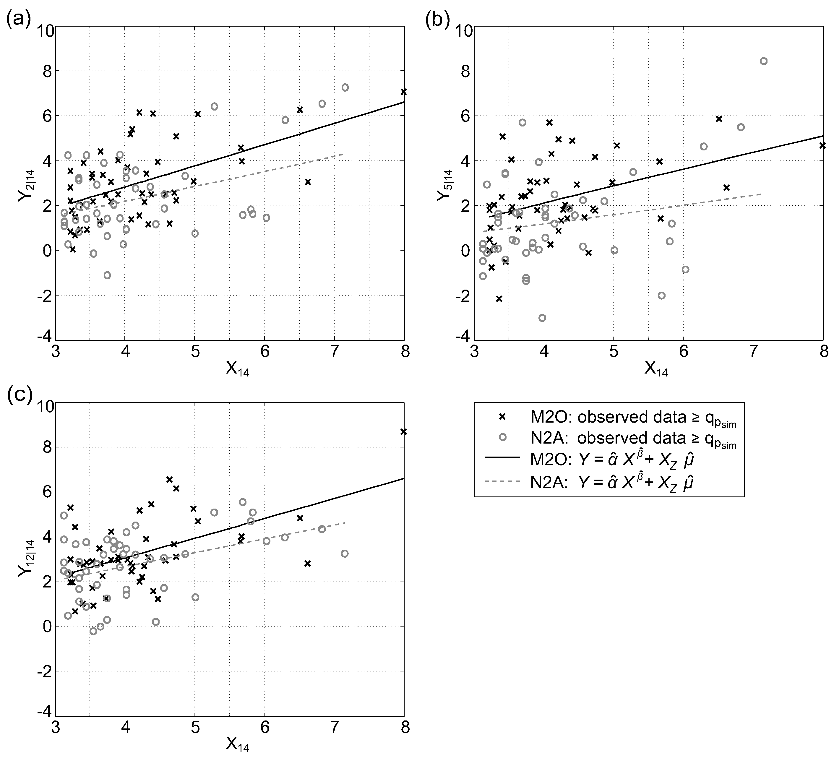
Figure 8.
Model application: (a) empirical CDF of number of extreme events i.e., at least one site exceeds ) per year and (b) probability that gauge i is most extreme.
Figure 8.
Model application: (a) empirical CDF of number of extreme events i.e., at least one site exceeds ) per year and (b) probability that gauge i is most extreme.

Figure 9.
Pairwise comparison of observed and simulated (-year) data of station Kennelbach (), Thal (), Gisingen (), and Schruns (). Upper triangle: . Lower triangle: .
Figure 9.
Pairwise comparison of observed and simulated (-year) data of station Kennelbach (), Thal (), Gisingen (), and Schruns (). Upper triangle: . Lower triangle: .

Figure 10.
Comparison of observed and simulated data of period for selected 17 sites. Medians of observed time series are depicted by blue crosses and medians of simulated data (100 × 38 year) are shown by selected percentiles.
Figure 10.
Comparison of observed and simulated data of period for selected 17 sites. Medians of observed time series are depicted by blue crosses and medians of simulated data (100 × 38 year) are shown by selected percentiles.
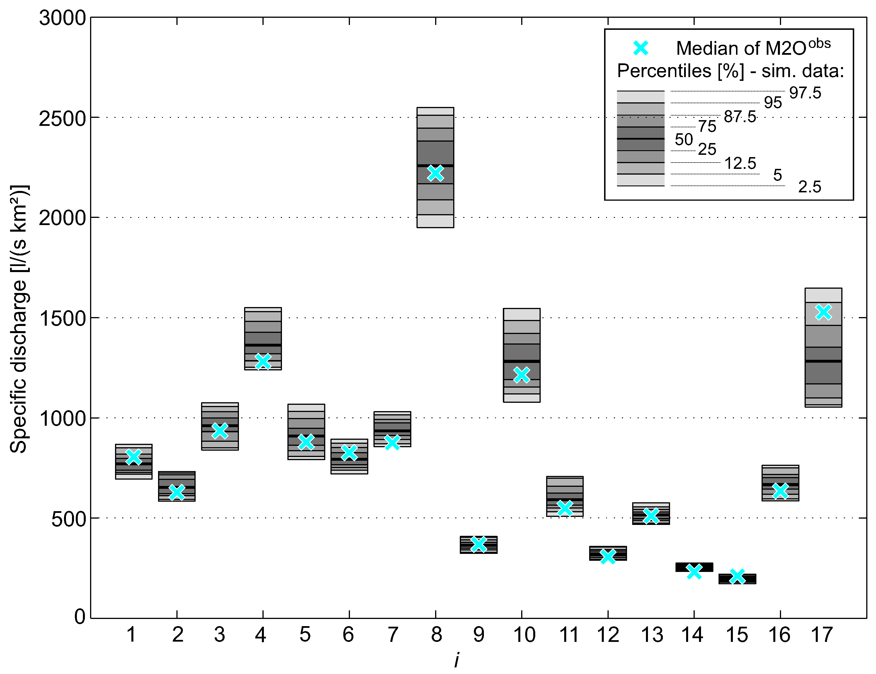
Figure 11.
Observed and examples of simulated flood events (T in year) including a categorization of the events severity by means of unit of flood hazard (UoFH).
Figure 11.
Observed and examples of simulated flood events (T in year) including a categorization of the events severity by means of unit of flood hazard (UoFH).


Table 1.
Selected River gauging stations, including the ID (station ID) according to the Austrian Hydrographic Service, and the catchment area (km2).
Table 1.
Selected River gauging stations, including the ID (station ID) according to the Austrian Hydrographic Service, and the catchment area (km2).
| i | Name of Gauges | River | ID | Area |
|---|---|---|---|---|
| 1 | Mellau | Bregenzerach | 200261 | 228.6 |
| 2 | Kennelbach | Bregenzerach | 200329 | 826.3 |
| 3 | Hopfreben | Bregenzerach | 200246 | 41.7 |
| 4 | Schönenbach | Subersach | 200287 | 31.1 |
| 5 | Thal | Rotach | 200311 | 90.1 |
| 6 | Lingenau | Subersach | 200295 | 111.6 |
| 7 | Hoher Steg | Dornbirnerach | 200212 | 112.9 |
| 8 | Enz | Dornbirnerach | 200204 | 51.1 |
| 9 | Lustenau (H) | Rheintalbinne | 200220 | 77.5 |
| 10 | Laterns | Frutz | 200154 | 33.4 |
| 11 | Unterhochsteg | Leiblach | 200394 | 102.4 |
| 12 | Schruns | Litz | 200048 | 102 |
| 13 | Garsella | Lutz | 200105 | 95.5 |
| 14 | Gisingen | Ill | 200147 | 1281 |
| 15 | Lustenau (E) | Rhein | 200196 | 6110 |
| 16 | Lech | Lech | 200378 | 84.3 |
| 17 | Lochau | Ruggbach | 200345 | 7.2 |
Table 2.
Probability that peaks (exceeding a threshold ) last L days.
| p | T (Year) | L (Days) | |||||
|---|---|---|---|---|---|---|---|
| 0 | 1 | 2 | 3 | 4 | |||
| R (p,L) | 0.99 | 0.3 | 1 | 0.32 | 0.21 | 0.03 | 0 |
| 0.997 | 0.9 | 1 | 0.39 | 0.25 | 0.02 | 0 | |
| 0.999 | 2.7 | 1 | 0.34 | 0.32 | 0.01 | 0 | |
| 0.9997 | 9.1 | 1 | 0.44 | 0.28 | 0 | 0 | |
Table 3.
Concentration time () and components and of ‘Burn vector’ based on for all sites.
| i | Name of Gauges | (h) | (°) | |
|---|---|---|---|---|
| 1 | Mellau | 1.9–4.8 | 204 | 0.56 |
| 2 | Kennelbach | 3.3–8.8 | 216 | 0.40 |
| 3 | Hopfreben | 0.7–2.3 | 205 | 0.52 |
| 4 | Schönenbach | 0.5–2.0 | 208 | 0.61 |
| 5 | Thal | 1.3–4.6 | 224 | 0.29 |
| 6 | Lingenau | 1.4–3.8 | 207 | 0.57 |
| 7 | Hoher Steg | 1.4–4.3 | 196 | 0.70 |
| 8 | Enz | 0.8–2.8 | 209 | 0.64 |
| 9 | Lustenau (H) | 1.4–8.7 | 190 | 0.73 |
| 10 | Laterns | 0.7–2.1 | 208 | 0.68 |
| 11 | Unterhochsteg | 1.0–6.3 | 188 | 0.45 |
| 12 | Schruns | 1.5–3.5 | 188 | 0.80 |
| 13 | Garsella | 1.2–3.0 | 200 | 0.69 |
| 14 | Gisingen | 5.3–12 | 192 | 0.76 |
| 15 | Lustenau (E) | 10–30 | 199 | 0.77 |
| 16 | Lech | 1.2–3.4 | 191 | 0.63 |
| 17 | Lochau | 0.4–1.3 | 205 | 0.58 |
Table 4.
Comparison of observed and simulated data for selected criteria ( and , and medians of yearly maximum runoff for summer and winter half-year). The results exhibit the proportion of possible combinations (, ) and sites (median()), respectively, where the observed data lies within the percentile range of simulated data.
| Test Criteria | Percentiles (%) | ||
|---|---|---|---|
| 12.5–87.5 | 5–95 | 2.5–97.5 | |
| 0.87 | 0.95 | 0.98 | |
| 0.91 | 0.97 | 0.99 | |
| 0.83 | 0.96 | 0.98 | |
| 0.87 | 0.98 | 0.99 | |
| median () | 0.71 | 0.94 | 0.94 |
| median () | 0.65 | 0.82 | 0.94 |
© 2018 by the authors. Licensee MDPI, Basel, Switzerland. This article is an open access article distributed under the terms and conditions of the Creative Commons Attribution (CC BY) license (http://creativecommons.org/licenses/by/4.0/).
Share and Cite
MDPI and ACS Style
Schneeberger, K.; Steinberger, T. Generation of Spatially Heterogeneous Flood Events in an Alpine Region—Adaptation and Application of a Multivariate Modelling Procedure. Hydrology 2018, 5, 5. https://doi.org/10.3390/hydrology5010005
AMA Style
Schneeberger K, Steinberger T. Generation of Spatially Heterogeneous Flood Events in an Alpine Region—Adaptation and Application of a Multivariate Modelling Procedure. Hydrology. 2018; 5(1):5. https://doi.org/10.3390/hydrology5010005
Chicago/Turabian StyleSchneeberger, Klaus, and Thomas Steinberger. 2018. "Generation of Spatially Heterogeneous Flood Events in an Alpine Region—Adaptation and Application of a Multivariate Modelling Procedure" Hydrology 5, no. 1: 5. https://doi.org/10.3390/hydrology5010005
Note that from the first issue of 2016, this journal uses article numbers instead of page numbers. See further details here.