Impact of Land Use Change on Flow and Sediment Yields in the Khokana Outlet of the Bagmati River, Kathmandu, Nepal

Texas Institute for Applied Environmental Research, 201 St. Felix St., BOX T-0410, Stephenville, TX 76402, USA
Hydrology 2018, 5(2), 22; https://doi.org/10.3390/hydrology5020022
Submission received: 25 January 2018
/
Revised: 23 March 2018
/
Accepted: 24 March 2018
/
Published: 28 March 2018
Abstract
:Land use changes are a key factor for altering hydrological response, and understanding its impacts can help to develop a sustainable and pragmatic strategy in order to preserve a watershed. The objective of this research is to estimate the impact of land use changes on Bagmati river discharge and sediment yield at the Khokana gauging station of the Kathmandu valley outlet. This study analyzes the impact of land use changes from the year 2000 to 2010 using a semi-distributed hydrological, Soil Water Assessment Tool (SWAT) model. The Load Estimator (LOADEST) simulates sediment loads on limited available sediment data. Sensitivity analysis is performed using the ParaSole (Parameter Solution) method within SWAT Calibration and Uncertainty Procedure (SWAT-CUP), which shows that Linear parameters for calculating the maximum amount of sediment that can be re-entrained during channel sediment routing is a most sensitive parameter that affect the hydrological response of the watershed. Monthly discharge and sediment data from 1995 to 2002 are used for calibration and remaining monthly discharge and sediment data from 2003 to 2010 are used for validation. Four statistical parameters including the Coefficient of Determination (R2), Nash–Sutcliffe Efficiency (NSE), RMSE-observations’ standard deviation ratio (RSR), and Percentage Bias (PBIAS) are estimated in order to evaluate the model performance. The results show a very good agreement between monthly measured and simulated discharge data as indicated by R2 = 0.88, NSE = 0.90, RSR = 0.34, and PBIAS = 0.03. The model shows nearly the same performance also with sediment data. The land use change data shows about a 6% increase in built-up areas from the years 2000 to 2010, whereas the remaining areas such as Forest, Shrub, Grass, Agriculture, Open Field, and Rivers/Lakes are decreased. The surface runoff contribution to stream flow and sediment yields are increased by 27% and 5% respectively. In the contrary, lateral flow contribution to stream flow and groundwater contribution to stream flow are decreased by 25% and 21%, respectively.
1. Introduction
Overexploiting natural resources for livelihood and economic activities is a common problem in developing countries Water resources are facing serious stress because of the rapid urbanization and soaring population growth rate, which has altered the hydrological response. Various hydrological indicators such as altering discharge, sediment, and nutrient yields can be used to investigate the impact of land use change. These indicators can be obtained either through on-site monitoring or using simulation models. On-site monitoring is generally unfeasible because it is labor intensive, time consuming, and expensive; therefore, the hydrological simulation model is gaining popularity to solve these problems. Selecting a proper model in the specific watershed has always been challenging, while field verification of the models’ parameters is useful to researchers in selecting the model for their purposes.
Land use change impacts various areas including hydrology, socio-economics, ecological, and environmental [1]. This is a triggering factor that leads to a change in the flow pattern due to the temporal variation of the discharge distribution [2]. Land use changes are a common problem in developing countries whose economies are generally based on agriculture [3]. Land use changes from agriculture to settlement alter the hydrological regime by increasing peak flow and decrease infiltration [4]. It accelerates soil erosion, which leads to various negative consequences such as increasing sedimentation, turbidity, and nutrients. Land use changes can lead to undesirable effects in the ecosystem, which cause water, soil, and air pollution [5].
The analysis of the land use change, which has an impact on the discharge, sediment, and nutrient yields, is enhanced by implementing modeling tools that incorporate both spatial and temporal dynamics. It is widely accepted that land use changes in the basin result in flooding, which is a major carrier of sediment [6]. The anthropogenic activities are mainly responsible for land use change in the river basin, and have been widely studied [7]. The hydrological model has become a useful tool in understanding the natural process in the river basin and its response of anthropogenic activities [8]. Geographic Information System (GIS)-based hydrological models are gaining popularity because of their capacity to easily incorporate spatial variability and estimate the land use change impact on the discharge. The GIS-based SWAT model is being used extensively in such conditions. SWAT has been widely used for simulating discharge, nutrient, and sediment from the basin [9,10]. This model has also shown to be an effective tool for assessing land use changes, water resources, and non-point pollution problems [11].
This paper is trying to evaluate the impact of land use change on the discharge, and sediment yields from the highly dense Kathmandu mountainous valley where approximately three million residents rely on the Bagmati river for their livelihoods and socioeconomic activities.
The influential factors of land use change are an increasing population, the expansion of urban areas, and climatic change, which is happening at alarming rates in Kathmandu. The expansion of built-up areas and overexploitation of natural resources to meet the demands of a soaring population will likely accelerate over the coming years. Therefore, scientific research is essential to estimate the impact of land use change on discharge. The finding of this research will disseminate knowledge to the policy makers to undertake effective measures for minimizing the undesirable impact of future land use change.
2. Methodology
2.1. Study Area
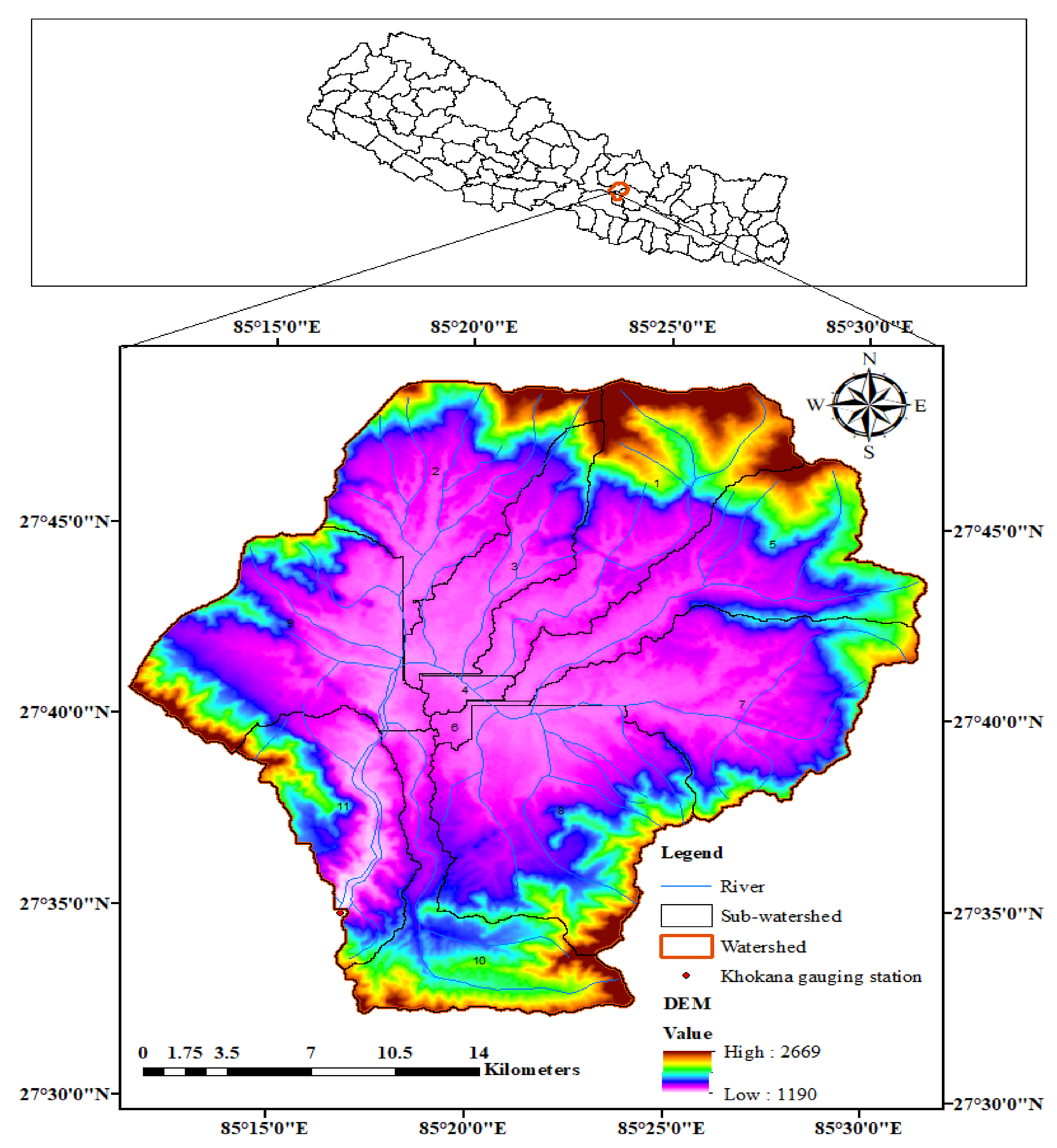
Bagmati is a medium-sized spring and monsoon rain-fed river flowing through the heart of the capital city, Kathmandu; it consists of many tributaries such as Bishnumati, Manohara, and Tukuchha (Figure 1).
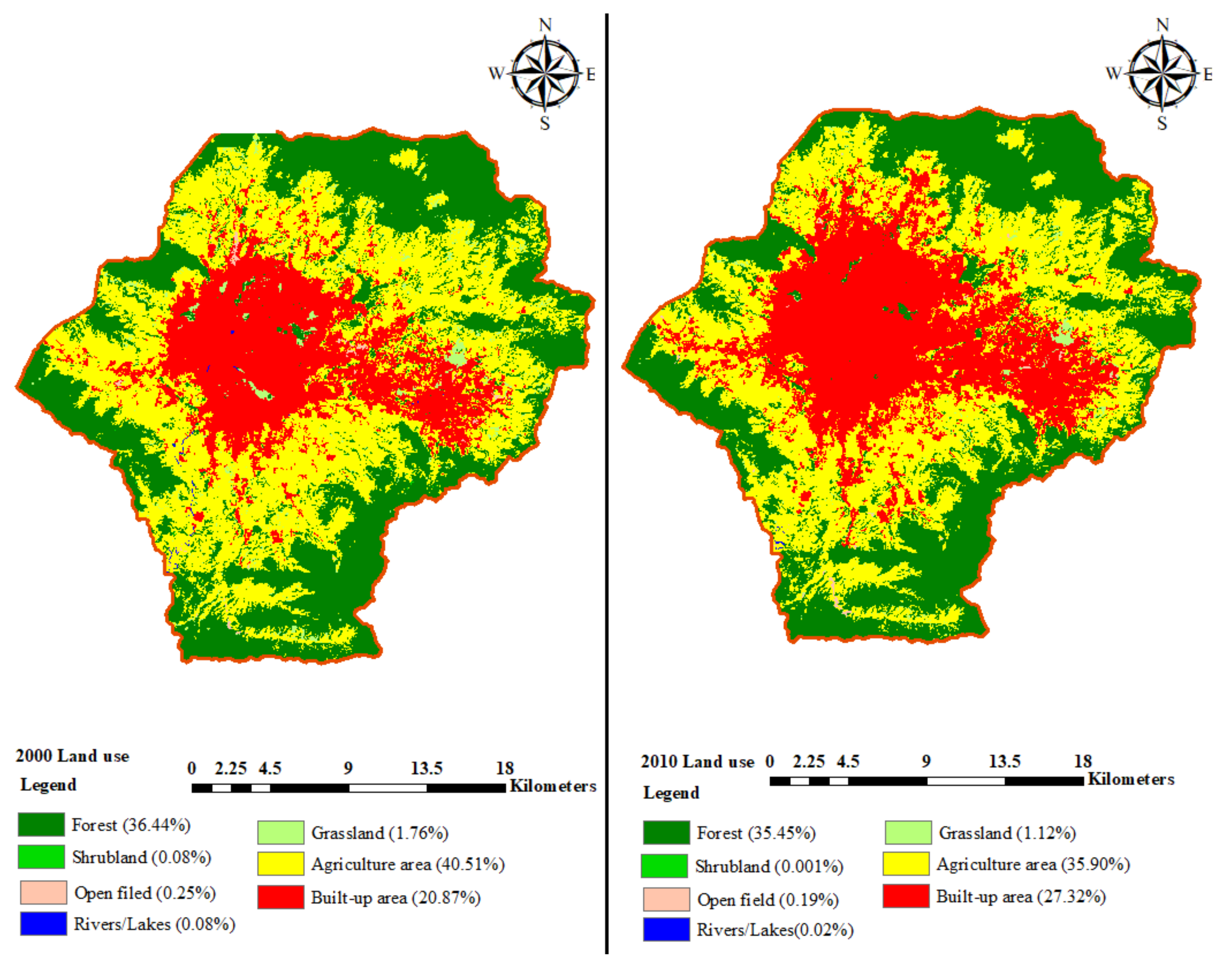
The Bagmati River originates at the Mahabharat Range of Shivapuri at an altitude 2669 m a.s.l. and has a catchment area at the Khokana gauging station that is 629 km2, which is situated at Latitude 27°37′44″, Longitude 85°17′41″, and 1190 m a.s.l. elevation. The mean monthly maximum air temperature reaches up to 29.3 °C and mean monthly minimum temperature reaches up to 0.9 °C. Likewise, the average annual rainfall is around 1300 mm [12]. In this research, the 2000 and 2010 years’ land use data are used in order to investigate its impact on the discharge and sediment yield. Comparing land use data of years 2000 and 2010, it shows that all classes of land use areas are decreased except the built-up areas, which have significantly increased from 131.26 km2 (20.87%) to 171.88 km2 (27.32%) (Table 1 and Figure 2). The study area is divided into 11 sub-watersheds, which vary from 3.12 km2 to 95.22 km2, followed by 49.49 km2 sub-watershed number 11, which is situated at the outlet and 118 Hydrologic Response Unit (HRU) based on soil and land use data.
2.2. SWAT Model
The SWAT model is used in this research in order to estimate the impact of land use change on discharge and sediment yield in the Bagmati river at the Khokana Gauging Station. SWAT is a conceptual, physically-based, semi-distributed hydrological model. This was developed in order to estimate the impact of land management practices on hydrology and water quality yields in large and complex watersheds having heterogeneous soil and land use conditions [13].
Runoff generation is an important part of the model that uses the Natural Resources Conservation Service (NRCS), and the formal Soil Conservation Service curve number (SCS-CN) method to calculate surface runoff and infiltration [14]. The CN depends on soil type, land use, and management practice, which distinguishes the amount of infiltration and surface runoff in a particular rain event. Higher CN value infers higher runoff and less infiltration [15]. The total discharge at the outlet is the discharge accumulated from each HRU, sub-surface flow, lateral flow, and return flow. The flow in SWAT is either routed through Muskingum or a variable storage coefficient method. Similarly, sediment yield from each HRU and erosion is estimated from the Modified Universal Soil Loss Equation (MUSLE), which uses a modification of Bagnold’s sediment transport equation for routing through the channel.
The GIS-based SWAT model has given researchers freedom to incorporate spatial variation and predict the hydrological process such as surface discharge, percolation, deep aquifer flow, evapotranspiration (ET), and channel routing [16]. The model strength for studying the long-term impact of land use change on discharge has given preference to select the SWAT model in this research. This is also a robust model for simulating sediment load and has been widely implemented in different parts of the world. The model performed well in monthly sediment loads rather than daily in the North Bosque River Watershed in North Texas [17]. The model divides the watershed into a number of sub-watersheds, which are connected by surface flow [18]. These sub-watersheds are further divided into number of hydrological response units (HRU) based on topography, land use, and soil input data. The model lumps the parameters into HRUs. Traditionally, HRUs are defined by the coincidence of soil type [19] and land use.
2.3. Model Setup
Data
The Digital Elevation Model (DEM), soils, land use, and weather are essential inputs data for the SWAT model. A Digital Elevation Map (DEM) of 30 m × 30 m resolution of the watershed was downloaded from NASA’s web site (https://reverb.echo.nasa.gov/reverb/). This is one of the critical input data required by the SWAT model to delineate the watershed and sub-watershed, and analyze the drainage pattern, slope, stream length, and width of the stream [20]. Land use maps of the years 2000 and 2010 are used to estimate the effect of land use change during these periods and were obtained from the International Centre for Integrated Mountain Development (ICIMOD, http://rds.icimod.org/). The soil data that defines the physical properties of the soil layers are obtained from the United State Department of Agriculture (https://www.nrcs.usda.gov/wps/portal/nrcs/detail/soils/survey/?cid=nrcs142p2_053627).
Discharge data of the Khokana Gauging Station and meteorological data such as daily rainfall, minimum and maximum temperature, solar radiation, wind speed, and relative humidity of the Kathmandu Airport and Khumaltar stations were obtained from the Department of Hydrology and Meteorology (DHM). Only 2003 to 2006 sediment concentration data are obtained from DHM, which are simulated to the calibration and validation period using LOADEST. The source and description of the data used in the SWAT model are highlighted in the Table 2.
2.4. Sensitivity Analysis
ParaSole (Parameter Solution) optimization method within the SWAT Calibration and Uncertainty Procedure (SWAT-CUP) is used for sensitivity analysis with 1000 trials. Sensitivity analysis is an important part of the model that reduces the number of parameters for calibration. This approach determines the most significant and sensitive parameters altering the water quantity and quality yields. The calibrated parameter range is used as a default parameter values in the Parasole. All parameters are selected for the sensitivity analysis. The results show that the SPCON is a most sensitive parameter (Rank 1) followed by EPCO, ESCO, GW_REVAP, SPEXP, REVAPMN, SOL_AWC, SURLAG, ALPHA_BF, RCHRG_DP, GW_DELAY, and CANMX. The remaining parameters have no significant effect on the stream flow and sediment simulation (Table 3).
SPCON is a linear parameter that estimates the maximum amount of sediment transports from the reach segment during the channel sediment routing, and an exponential parameter (SPEXP) is for calculating sediment re-entrained. These parameters affect the movement and separation of the sediment fraction in the reach and are adjusted within their acceptable limit to match the measured sediment yield. Baseflow recession coefficient (ALPHA_BF) is a direct index of the groundwater flow response to change in recharge [21]. This factor determines the ratio corresponding to the base and surface flow contribution to the total flow. GW_DELAY is a lag time between water exiting from the soil profile and entering the shallow aquifer. Deep aquifer percolation fraction (RCHRG_DP) is a fraction from the root zone that recharges the deep aquifer. Plant uptake compensation factor (EPCO) shows the relation between water uptake by the plant to meet its transpiration demand and the amount of water available in the soil.
ESCO adjusts the evaporation depth distribution of the soil in order to show the effect of capillary action, crusting, and cracking [18]. GW_REVAP explains that the fraction of water that can be moved from a shallow aquifer into the overlaying unsaturated soil layer is a function of evapotranspiration. REVAPMN is a threshold water depth in the aquifer for “revap” or percolation to a deep aquifer. SOL_AWC is a key soil parameter associated with generating runoff and evaporation [22]. A higher value of it infers a higher water holding capacity of soil, which means less water available for the surface runoff and percolation. SURLAG is a sub-watershed level parameter and controls the fraction of the total water available that is allowed to enter the stream in a specific time period. CANMX is the maximum canopy storage that significantly affects infiltration, runoff, and evapotranspiration because of reduction in the erosive energy of droplets and traps a portion of the rainfall within the canopy.
2.5. Model Calibration and Validation
The model performance is generally evaluated with the data collected at the outlet of the watershed. Bagmati River in Khokana is only an outlet of Kathmandu Valley and is a sampling site. Daily discharge and few years sediment concentration data are obtained from DHM. Sediment data are simulated to the entire calibration and validation period using the LOADEST regression model [23]. This regression model simulates nutrients and sediment load in the discharge using time series discharge and constituent concentration data as inputs. This model is widely accepted for simulating load from a limited amount of nutrient and sediment data. Monthly time step discharge and sediment data are used for calibration and validation.
In order to understand the uncertainty characters of the basin, three years (1992 to 1994) of data are used for the warm up period. Monthly data from 1995 to 2002 are used for calibration and remaining data of from 2003 to 2010 are used for validation. Calibrated parameters of the model are shown in Table 3. Manual calibration and validation techniques are adopted by varying parameters within their acceptable ranges, assuming that the optimal set of parameters exists for the model for describing hydrology of the study area that is shown by the good agreement between measured and simulated data both in calibration and validation period with discharge and sediment data. This is accomplished by comparing the measured data with the SWAT output of the same duration [24]. Model robustness and performance are evaluated both in the calibration and validation graphically and quantified using statistical parameters [25]. These statistical parameters are: Coefficient of determination (R2), Nash–Sutcliffe simulation efficiency (NSE), RMSE-observations standard deviation ratio (RSR), and Percentage of Bias (PBIAS) [26]. The coefficient of determination (R2) explains the degree of collinearity between the measured and simulated data [27]. Typically, R2 greater than 0.5 is considered an acceptable limit for model performance [28,29]. The model performance is classified as very good, good, satisfactory, and unsatisfactory if the NSE value is larger than 0.75, between 0.65 and 0.75, between 0.5 and 0.65, and less than 0.5, respectively [27]. The zero RMSE value indicates perfect agreement between measured and simulated data. RMSE less than 0.5 of standard deviation of the measured data indicates good model performance [30,31]. PBIAS indicates the average tendency of the simulated data to be larger or smaller than the observed data. Its zero value indicates perfect matching of measured and simulated data. Positive values indicate underestimation bias and negative value indicates overestimation bias [32].
3. Results and Discussion
In the calibration period, the model was unable to capture the peak of measured discharge. In contrast, the model over-forecasts the peak discharge in the validation period. This problem may be increasing in built up area creates impervious layers which reduces infiltration and percolation that cause increases in surface runoff. This is probably a shortcoming of the SWAT model for forecasting the hydrograph of the present watershed. However, results indicate the good agreement between the measured and simulated discharge for both calibration and validation periods. The statistical parameters R2, NSE, RSR, and PBIAS are estimated as 0.88, 0.90, 0.34, and 0.03 in calibration, and 0.86, 0.72, 0.53, and −0.25 in the validation period, respectively (Table 4). These values indicate a very good level of model performance with the discharge data. The graphical comparison of measured and simulated discharge data during calibration and validation period, regression analysis for finding R2, and comparison of the yearly discharge data are shown in Figure 3, Figure 4 and Figure 5, respectively.
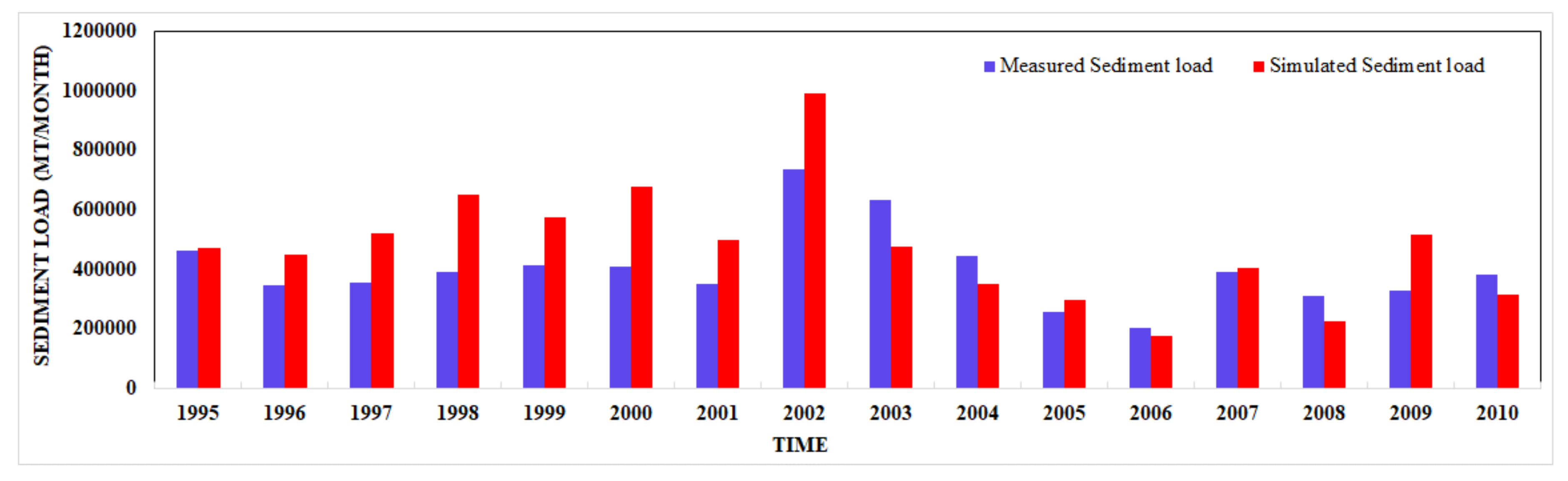
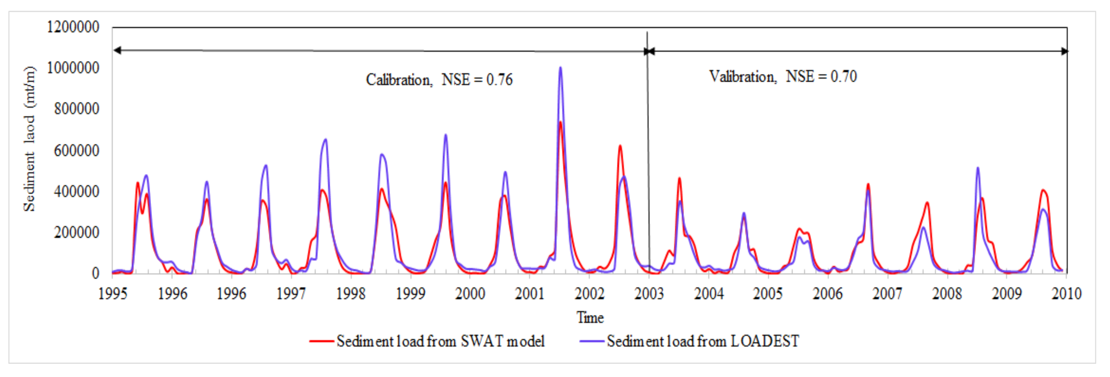
Similarly to the discharge, the performance of SWAT model is also evaluated graphically and statistically with the monthly sediment data. The graphical comparison of monthly sediment data during calibration and validation period, regression analysis for finding R2, and comparison of the yearly sediment data are shown in Figure 6, Figure 7 and Figure 8, respectively. Table 5 shows statistical parameters estimated in order to evaluate the SWAT performance with the sediment data, which shows 0.84, 0.76, 0.49, and 0.30 in calibration and 0.73, 0.70, 0.55, and −0.21 in validation, respectively. The statistical parameters indicate that the SWAT model shows a very good level of performance also with sediment data. Four parameters such as CH_EROD, SPCON, SPEXP, and CH-COV are mainly adjusted to their default limit in order to match the LOADEST simulated sediment load with the SWAT simulated (Table 3).
Table 3 indicates the list of parameters adjusted during calibration with discharge and sediment data. Land use data of 2000 and 2010 show some noteworthy changes in the land use classes. The results show that, during these periods, all land use classes (Forest, Shrub, Grass, Agriculture, Open Field, and Rivers/Lakes) are reduced by 40.62 km2 (6.46%), which are converted to Built-Up Areas. The impact of land use change is estimated by running the model using 2000 land use along with climate data from 1992 to 2002 and using 2010 land use along with climate data from 2000 to 2010 keeping the parameters, DEM, and Soil data constant.
The research has found the greatest impact on the surface runoff contribution to stream flow, which is increased from 172 mm/year to 219 mm/year, representing 27% (Table 6). The built-up areas increase by 40.62 km2 (6.46%) is attributed to the increasing surface runoff contribution to stream flow. The increase in built-up areas creates impervious layers, which reduces infiltration and percolation that cause increases in surface runoff. This finding supports the statement that an increase in built-up areas increases impervious surfaces, which accelerates surface runoff [33,34].
Lateral flow contribution to stream flow is decreased from 455 mm/year to 340 mm/year, representing 25%. Sediment yield is increased from 2.99 mt/ha to 3.15 mt/ha, representing 5%, which is supported by the Wolman statement as the urban landscape is built out, the sediment yield increase [35]. In the contrast, groundwater contribution to stream flow is decreased from 391 mm/year to 309 mm/year (21%). This is attributed to less soil infiltration and more surface runoff, and an increasing rate of groundwater abstraction from the shallow and deep aquifer for water supply and irrigation. These scenarios are happening in the research area and are expected to accelerate in the future.
4. Conclusions
In this research, a GIS-based SWAT model is used to estimate the impact of land use changes on the discharge and sediment yield of the Bagmati river at the Khokana Gauging Station in Nepal. Online data sources are used to download DEM, Soil, and Land use data, whereas discharge and meteorological data are obtained from the Department of Hydrology and Meteorology (DHM). Data from 1992 to 1994 are used for the warm up period, whereas 1995 to 2002 data are used for calibration and the remaining 2003 to 2010 data are used for validation. Four statistical parameters (R2, NSE, RSR, and PBIAS) are used to evaluate the level of agreement between measured and simulated discharge and sediment data, which are estimated as 0.88, 0.90, 0.34, and 0.03 in the calibration period and 0.86, 0.72, 0.53, and −0.25 in the validation period, respectively, with the discharge date. Nearly similar model performances are also achieved with the sediment data. These values indicate that the model performs very well both with the discharge and sediment data. Comparison of land use data between 2000 and 2010 shows the noteworthy land use changes where all the land use classes are decreased except built-up areas, which are increased by 40.62 km2 (6.46%). Therefore, surface water contribution to stream flow and sediment yields is increased by 27% and 5%, respectively. It is believed that expansion of the urban attributes increases surface water contribution to stream flow, which carries more sediment. In the contrast, groundwater contribution to stream flow is decreased by 25% because of decreasing infiltration due to the expansion of urban areas.
The continuation of land use change is a serious threat in the Bagmati Watershed. Due to continuous sediment accumulation, the river bed has been risen. Therefore, small flood is more likely to topple the river and are become a too serious threats to the residents particularly in the low land, and impact on their economic activities. Contamination of the river due to the direct disposal of effluent and sewerage results in extinction of aquatic life and leads to a serious threat for those downstream who are dependent on the river for their livelihood. Therefore, a sustainable and pragmatic strategy should be developed in order to preserve the watershed. A well-calibrated SWAT model can simulate discharge and sediment related to the impact of land use change, which is expected to be a valuable asset and information to the policy makers.
Acknowledgments
My special thanks go to my colleagues, Narayan Kannan and Rewari Niruala for their valuable suggestions in order to accomplish this research. My thanks also go to DHM for providing valuable hydro-met data and those who supported me directly and indirectly to accomplish this research.
Conflicts of Interest
The author declares no conflicts of interest.
References
- Ndulue, E.L.; Mbajiorgu, C.C.; Ugwu, S.N.; Ogwo, V.; Ogbu, K.N. Assessment of Land Use/cover Impacts on Runoff and Sediment Yield Using Hydrologic Models: A Review. J. Ecol. Nat. Environ. 2015, 7, 46–55. [Google Scholar] [CrossRef]
- Kashaigili, J.J. Impacts of land-use and land-cover changes on flow regimes of the Usangu Wetland and the Great Ruaha River, Tanzania. Phys. Chem. Earth Parts A/B/C 2008, 33, 640–647. [Google Scholar] [CrossRef]
- Tufa, D.F.; Abbulu, Y.; Srinivasarao, G.V.R. Watershed Hydrological Response to Changes in Land Use/Land Covers Patterns of River Basin: A Review. Int. J. Civ. Struct. Environ. Infrastruct. Eng. Res. Dev. 2014, 4, 157–170. [Google Scholar]
- Sahin, V.; Hall, M.J. The Effects of Afforestation and Deforestation on Water Yields. J. Hydrol. 1996, 178, 293–309. [Google Scholar] [CrossRef]
- Jokar Arsanjani, J.; Helbich, M.; Bakillah, M.; Hagenauer, J.; Zipf, A. Toward Mapping Land-Use Patterns from Volunteered Geographic Information. Int. J. Geogr. Inf. Sci. 2013, 27, 2264–2278. [Google Scholar] [CrossRef]
- Zhang, X.; Wenhong, C.; Qingchao, G.; Sihong, W. Effects of Landuse Change on Surface Runoff and Sediment Yield at Different Watershed Scales on the Loess Plateau. Int. J. Sediment Res. 2010, 25, 283–293. [Google Scholar] [CrossRef]
- Nearing, M.A.; Jetten, V.G.; Baffaut, C.; Cerdan, O.; Couturier, A.; Hernandez, M.; Le Bissonnais, Y.; Nichols, M.H.; Nunes, J.P.; Renschler, C.S.; et al. Modeling Response of Soil Erosion and Runoff to Changes in Precipitation and Cover. Catena 2005, 61, 131–154. [Google Scholar] [CrossRef]
- Setegn, S.G.; Srinivasan, R.; Dargahi, B. Hydrological Modelling in the Lake Tana Basin, Ethiopia Using SWAT Model. Open Hydrol. J. 2008, 2, 49–62. [Google Scholar] [CrossRef]
- Kirsch, K.; Kirsch, A.; Arnold, J.G. Predicting Sediment and Phosphorus Loads in the Rock River Basin Using SWAT. Forest 2002, 45, 1757–1769. [Google Scholar] [CrossRef]
- Spruill, C.A.; Workman, S.R.; Taraba, J.L. Simulation of Daily and Monthly Stream Discharge from Small Watersheds Using the SWAT Model. Trans. ASAE 2000, 43, 1431–1439. [Google Scholar] [CrossRef]
- Arnold, J.G.; Srinivasan, R.; Muttiah, R.S.; Williams, J.R. Large Area Hydrologic Modeling and Assessment Part II: Model Application. J. Am. Water Resour. Assoc. 1998, 34, 91–101. [Google Scholar] [CrossRef]
- Upadhyay, A.K.; Yoshida, H.; Rijal, H.B. Climate Responsive Building Design in the Kathmandu Valley. J. Asian Archit. Build. Eng. 2006, 5, 169–176. [Google Scholar] [CrossRef]
- Arnold, J.G.; Srinivasan, R.; Muttiah, R.S.; Williams, J.R. Large Area Hydrologic Modeling and Assessment Part I: Model Development. J. Am. Water Resour. Assoc. 1998, 34, 73–89. [Google Scholar] [CrossRef]
- Boughton, W.C. A Review of the USDA SCS Curve Number Method. Soil Res. 1989, 27, 511–523. [Google Scholar] [CrossRef]
- Zhang, H.; Huang, G.H.; Wang, D.; Zhang, X. Multi-Period Calibration of a Semi-Distributed Hydrological Model Based on Hydroclimatic Clustering. Adv. Water Resour. 2011, 34, 1292–1303. [Google Scholar] [CrossRef]
- Wu, K.; Xu, Y.J. Evaluation of the Applicability of the SWAT Model for Coastal Watersheds in Southeastern Louisiana. J. Am. Water Resour. Assoc. 2006, 42, 1247–1260. [Google Scholar] [CrossRef]
- Saleh, A.; Arnold, J.G.; Gassman, P.W.A.; Hauck, L.M.; Rosenthal, W.D.; Williams, J.R.; McFarland, A.M.S. Application of SWAT for the Upper North Bosque River Watershed. Trans. ASAE 2000, 43, 1077–1087. [Google Scholar] [CrossRef]
- Neitsch, S.L.; Arnold, J.G.; Kiniry, J.E.A.; Srinivasan, R.; Williams, J.R. Soil and Water Assessment Tool User’s Manual Version 2000; GSWRL Report 202(02-06); GSWRL: Temple, TX, USA, 2002. [Google Scholar]
- Rawls, W.J.; Brakensiek, D.L.; Saxtonn, K.E. Estimation of Soil Water Properties. Trans. ASAE 1982, 25, 1316–1320. [Google Scholar] [CrossRef]
- Chaplot, V. Impact of DEM Mesh Size and Soil Map Scale on SWAT Runoff, Sediment, and NO3–N Loads Predictions. J. Hydrol. 2005, 312, 207–222. [Google Scholar] [CrossRef]
- Smedema, L.K.; Rycroft, D.W. Land Drainage: Planning and Design of Agricultural Systems; Batsford Academic and Educational Ltd.: London, UK, 1983. [Google Scholar]
- Burba, G.G.; Verma, S.B. Seasonal and Interannual Variability in Evapotranspiration of Native Tallgrass Prairie and Cultivated Wheat Ecosystems. Agric. For. Meteorol. 2005, 135, 190–201. [Google Scholar] [CrossRef]
- Runkel, R.L.; Crawford, C.G.; Cohn, T.A. Load Estimator (LOADEST): A FORTRAN Program for Estimating Constituent Loads in Streams and Rivers; CreateSpace Independent Publishing Platform: New York, NY, USA, 2004. [Google Scholar]
- Arnold, J.G.; Moriasi, D.N.; Gassman, P.W.; Abbaspour, K.C.; White, M.J.; Srinivasan, R.; Santhi, C.; Harmel, R.D.; van Griensven, A.; van Liew, M.W.; et al. SWAT: Model Use, Calibration, and Validation. Trans. ASABE 2012, 55, 1491–1508. [Google Scholar] [CrossRef]
- Betrie, G.D.; Mohamed, Y.A.; van Griensven, A.; Srinivasan, R. Sediment Management Modelling in the Blue Nile Basin Using SWAT Model. Hydrol. Earth Syst. Sci. 2011, 15, 807–818. [Google Scholar] [CrossRef]
- Fukunaga, D.C.; Cecílio, R.A.; Zanetti, S.S.; Oliveira, L.T.; Caiado, M.A.C. Application of the SWAT Hydrologic Model to a Tropical Watershed at Brazil. Catena 2015, 125, 206–213. [Google Scholar] [CrossRef]
- Moriasi, D.N.; Arnold, J.G.; Van Liew, M.W.; Bingner, R.L.; Harmel, R.D.; Veith, T.L. Model Evaluation Guidelines for Systematic Quantification of Accuracy in Watershed Simulations. Trans. ASABE 2007, 50, 885–900. [Google Scholar] [CrossRef]
- Van Liew, M.W.; Arnold, J.G.; Garbrecht, J.D. Hydrologic Simulation on Agricultural Watersheds: Choosing between Two Models. Trans. ASAE 2003, 46, 1539–1551. [Google Scholar] [CrossRef]
- Santhi, C.; Arnold, J.G.; Williams, J.R.; Dugas, W.A.; Srinivasan, R.; Hauck, L.M. Validation of the Swat Model on a Large Rwer Basin with Point and Nonpoint Sources. J. Am. Water Resour. Assoc. 2011, 37, 1169–1188. [Google Scholar] [CrossRef]
- Singh, J.; Knapp, H.V.; Arnold, J.G.; Demissie, M. Hydrological Modeling of the Iroquois River Watershed Using HSPF and SWAT. J. Am. Water Resour. Assoc. 2005, 41, 343–360. [Google Scholar] [CrossRef]
- Vazquez-Amábile, G.G.; Engel, B.A. Use of SWAT to Compute Groundwater Table Depth and Streamflow in the Muscatatuck River Watershed. Trans. ASAE 2005, 48, 991–1003. [Google Scholar] [CrossRef]
- Gupta, H.V.; Sorooshian, S.; Yapo, P.O. Status of Automatic Calibration for Hydrologic Models: Comparison with Multilevel Expert Calibration. J. Hydrol. Eng. 1999, 4, 135–143. [Google Scholar] [CrossRef]
- Nie, W.; Yuan, Y.; Kepner, W.; Nash, M.S.; Jackson, M.; Erickson, C. Assessing Impacts of Landuse and Landcover Changes on Hydrology for the Upper San Pedro Watershed. J. Hydrol. 2011, 407, 105–114. [Google Scholar] [CrossRef]
- Tang, Z.; Engel, B.A.; Pijanowski, B.C.; Lim, K.J. Forecasting Land Use Change and Its Environmental Impact at a Watershed Scale. J. Environ. Manag. 2005, 76, 35–45. [Google Scholar] [CrossRef] [PubMed]
- Wolman, M.G. A Cycle of Sedimentation and Erosion in Urban River Channels. Geogr. Ann. Ser. A Phys. Geogr. 1967, 49, 385–395. [Google Scholar] [CrossRef]
Figure 1.
Location map of the study area.

Figure 2.
Land use classified map of the Bagmati Watershed at the Khokana Gauging Station.

Figure 3.
Observed and simulated monthly discharge data of Bagmati Watershed at the Khokana Gauging Station.
Figure 3.
Observed and simulated monthly discharge data of Bagmati Watershed at the Khokana Gauging Station.
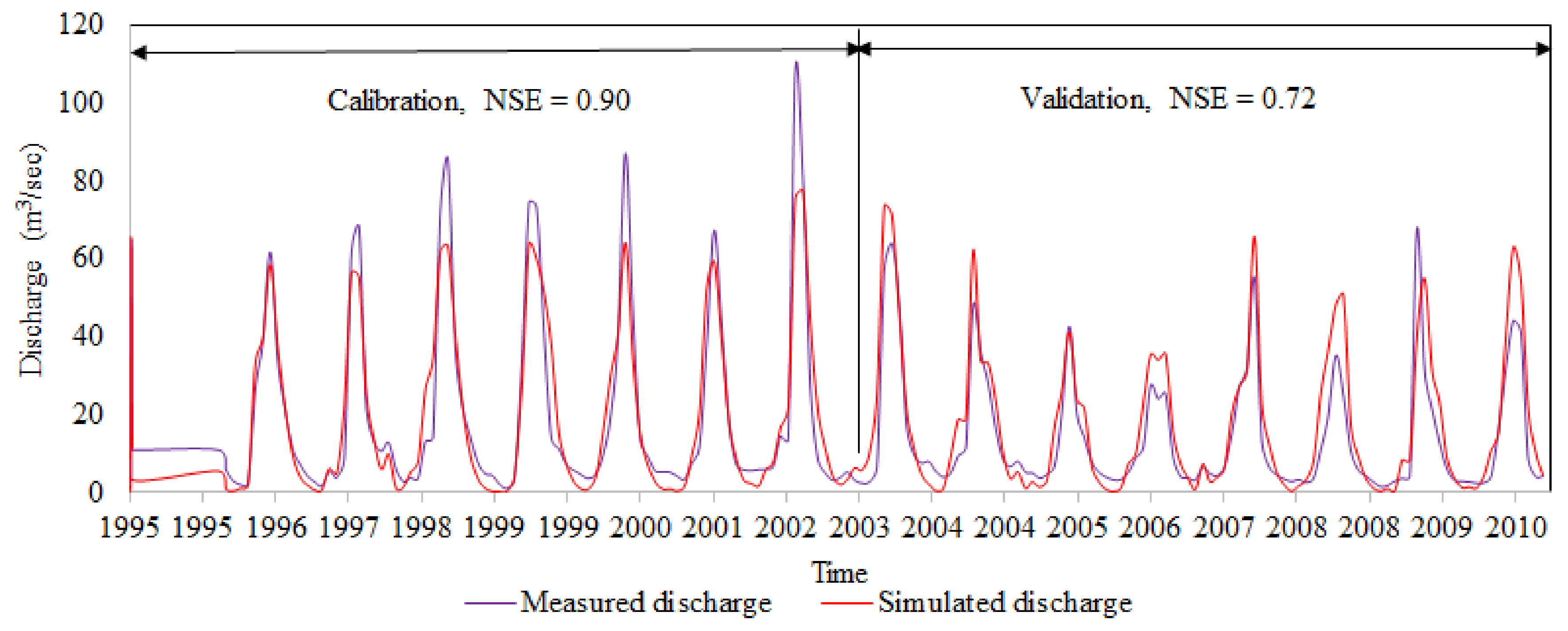
Figure 4.
Scatter plots of observed and simulated monthly discharge data of the calibration and validation period.
Figure 4.
Scatter plots of observed and simulated monthly discharge data of the calibration and validation period.
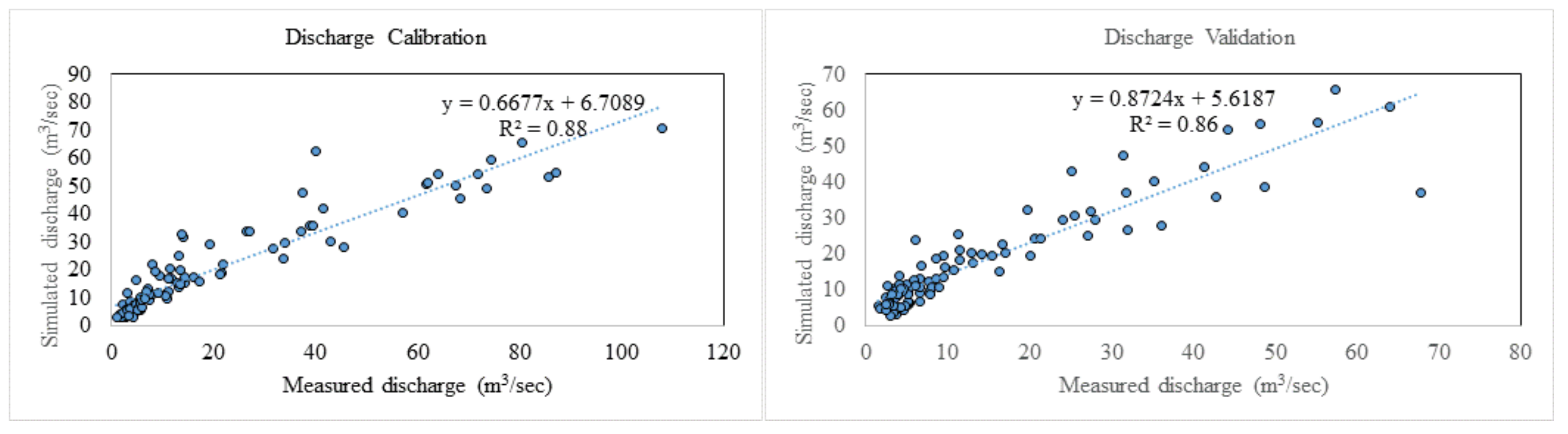
Figure 5.
The relationship between the calibrated and simulated yearly discharge data.

Figure 6.
Observed and simulated monthly sediment load of Bagmati Watershed at the Khokana Gauging Station.
Figure 6.
Observed and simulated monthly sediment load of Bagmati Watershed at the Khokana Gauging Station.

Figure 7.
Scatter plots of observed and simulated monthly sediment data in the calibration and validation period.
Figure 7.
Scatter plots of observed and simulated monthly sediment data in the calibration and validation period.
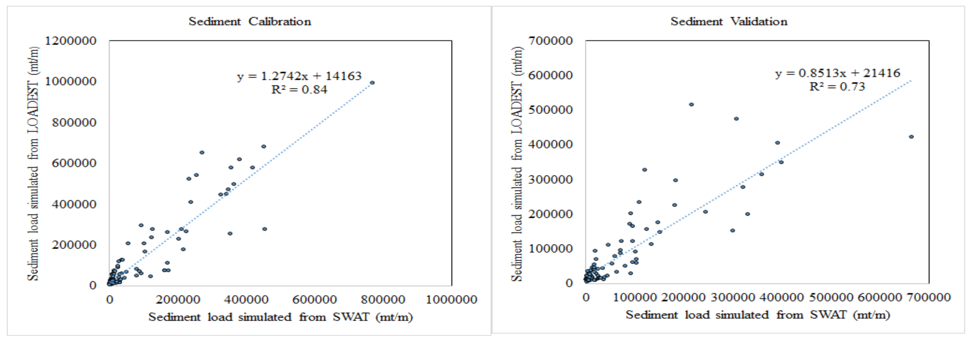
Figure 8.
The relationship between the calibrated and simulated yearly sediment data.

Table 1.
Land use classes in the Bagmati watershed at Khokana gauging station.
| Land Use | ||||||
|---|---|---|---|---|---|---|
| 2000 | 2010 | Difference | ||||
| Area (km2) | % | Area (km2) | % | km2 | % | |
| Forest | 229.23 | 36.44 | 223.00 | 35.45 | −6.23 | −0.99 |
| Shrubland | 0.53 | 0.08 | 0.005 | 0.001 | −0.53 | −0.08 |
| Grassland | 11.08 | 1.76 | 7.02 | 1.12 | −4.06 | −0.65 |
| Agriculture | 254.85 | 40.51 | 225.83 | 35.90 | −29.03 | −4.61 |
| Open Field | 1.57 | 0.25 | 1.21 | 0.19 | −0.35 | −0.06 |
| Rivers/Lakes | 0.53 | 0.08 | 0.12 | 0.02 | −0.41 | −0.07 |
| Built-Up Areas | 131.26 | 20.87 | 171.88 | 27.32 | 40.62 | 6.46 |
| Total | 629.05 | 629.05 | ||||
Table 2.
Input data for the SWAT model at Khokana gauging station.
| Data | Duration | Resolution | Source |
|---|---|---|---|
| Digital Elevation Model (DEM) | 30 m × 30 m | NASA | |
| Land use | 2000 and 2010 | ICIMOD | |
| Soil | 2000 | NASA | |
| Meteorological data of Kathmandu airport and Khumaltar | 1992–2010 | DHM | |
| Discharge data of Khokana gauging station | 1995–2010 | DHM | |
| Sediment data of Khokana gauging station | 2003–2006 | DHM |
Table 3.
List of calibrated parameters and their values.
| Calibration | |||||
|---|---|---|---|---|---|
| Parameters | Definition | Unit | Range of Values | Calibrated | Rank |
| SPCON(.bsn) | Linear parameter for calculating the maximum amount of sediment that can be reentrained during channel sediment rounting | 0.0001 to 0.01 | 0.01 | 1 | |
| EPCO(.hru) | Plant uptake compensation factor | 0.01 to 1 | 0.1 | 2 | |
| ESCO(.hru) | Soil evaporation compensation factor | 0.01 to 1 | 0.1 | 3 | |
| GW_REVAP(.gw) | Groundwater revap coefficient | 0.02 to 0.2 | 0.02 | 4 | |
| SPEXP(.bsn) | Exponent parameter for calculating sediment re-entrained in channel sediment routing | 1 to 2 | 0.72 | 5 | |
| REVAPMN(.gw) | Threshold depth of water in the shallow aquifer for “revap” or percolation to the deep aquifer | 0 to 500 | 100 | 6 | |
| SOIL_AWC(.sol) | Available soil water capacity | 0-0.12 | 0.02 | 7 | |
| SURLAG(.bsn) | Surface runoff lag coefficient | day | 1 to 12 | 5 | 8 |
| APHA_BF(.gw) | Baseflow alpha factor for recession constant | 0 to 1 | 0.048 | 9 | |
| RECHRG-DP(.gw) | Deep aquifer percolation fraction | 0 to 1 | 0.05 | 10 | |
| GW_DELAY(.gw) | Groundwater delay | day | 0 to 500 | 31 | 11 |
| CANMX(.hru) | Maximum canopy storage | 0 to 100 | 1 | 12 | |
| CH-N2(.mgt) | Manning’s roughness coefficient for the main channel | 0 to 0.1 | 0.1 | 13 | |
| GWQMN(.gw) | Threshold depth of water in the shallow aquifer for return flow | 0 to 5000 | 1000 | 14 | |
| CN2(.mgt) | SCS runoff curve number | 39 to 98 | ±10 | 15 | |
| CH-K2(.rte) | Effective hydraulic conductivity in the main channel | 0 to 150 | 2 | 16 | |
| CH-EROD(.rte) | Channel erodibility factor | 0 to 1 | 0.18 | 17 | |
| CH-COV(.rte) | Channel cover factor | 0 to 1 | 0.18 | 18 | |
Table 4.
Calibration and Validation statistics of the SWAT model using monthly discharge data.
| Stage of Model | Evaluated Statistics | |||
|---|---|---|---|---|
| R2 | NSE | RSR | PBIAS | |
| Calibration (1995–2002) | 0.88 | 0.90 | 0.34 | 0.03 |
| Validation (2003–2010) | 0.86 | 0.72 | 0.53 | −0.25 |
Table 5.
Calibration and validation statistics of the SWAT model using monthly sediment data.
| Stage of Model | Evaluated Parameters | |||
|---|---|---|---|---|
| R2 | NSE | RSR | PBIAS | |
| Calibration (1995–2002) | 0.85 | 0.76 | 0.49 | 0.30 |
| Validation (2003–2010) | 0.73 | 0.70 | 0.55 | −0.21 |
Table 6.
Estimated discharge, sediment yield at different land uses.
| Component | Land Use | % Change | |
|---|---|---|---|
| 2000 | 2010 | ||
| Surface runoff contribution to stream flow SURQ (mm/year) | 171.99 | 219.17 | +27.43 |
| Lateral flow contribution to stream flow LATQ (mm/year) | 455.51 | 340.14 | −25.33 |
| Ground water contribution to stream flow (mm/year) | 390.66 | 309.09 | −20.88 |
| Sediment yield (mt/ha) | 2.99 | 3.15 | +5.41 |
© 2018 by the author. Licensee MDPI, Basel, Switzerland. This article is an open access article distributed under the terms and conditions of the Creative Commons Attribution (CC BY) license (http://creativecommons.org/licenses/by/4.0/).
Share and Cite
MDPI and ACS Style
Pokhrel, B.K. Impact of Land Use Change on Flow and Sediment Yields in the Khokana Outlet of the Bagmati River, Kathmandu, Nepal. Hydrology 2018, 5, 22. https://doi.org/10.3390/hydrology5020022
AMA Style
Pokhrel BK. Impact of Land Use Change on Flow and Sediment Yields in the Khokana Outlet of the Bagmati River, Kathmandu, Nepal. Hydrology. 2018; 5(2):22. https://doi.org/10.3390/hydrology5020022
Chicago/Turabian StylePokhrel, Bijay K. 2018. "Impact of Land Use Change on Flow and Sediment Yields in the Khokana Outlet of the Bagmati River, Kathmandu, Nepal" Hydrology 5, no. 2: 22. https://doi.org/10.3390/hydrology5020022
Note that from the first issue of 2016, this journal uses article numbers instead of page numbers. See further details here.