Skill Transfer from Meteorological to Runoff Forecasts in Glacierized Catchments


1
Swiss Federal Institute for Forest, Snow and Landscape Research WSL, CH-8903 Birmensdorf, Switzerland
2
Laboratory of Hydraulics, Hydrology and Glaciology (VAW), ETH Zurich, CH-8903 Zurich, Switzerland
*
Author to whom correspondence should be addressed.
Hydrology 2018, 5(2), 26; https://doi.org/10.3390/hydrology5020026
Submission received: 13 March 2018
/
Revised: 9 May 2018
/
Accepted: 10 May 2018
/
Published: 15 May 2018
(This article belongs to the Special Issue Climatic Change Impact on Hydrology)
Abstract
:Runoff predictions are affected by several uncertainties. Among the most important ones is the uncertainty in meteorological forcing. We investigated the skill propagation of meteorological to runoff forecasts in an idealized experiment using synthetic data. Meteorological forecasts with different skill were produced with a weather generator and fed into two different hydrological models. The experiments were repeated for two glacierized catchments of different sizes and morphological characteristics, and for scenarios of different glacier coverage. The results show that for catchments with high glacierization (>50%), the runoff forecast skill is more dependent on the skill of the temperature forecasts than the one for precipitation. This is because snow and ice melt are strongly controlled by temperature. The influence of the temperature forecast skill diminishes with decreasing glacierization, while the opposite is true for precipitation. Precipitation starts to dominate the runoff skill when the catchment’s glacierization drops below 30%, or when the total contribution of ice and snow melt is less than about 60%. The skill difference between meteorological forecasts and runoff predictions proved to be independent from the lead time, and all results were similar for both the considered hydrological models. Our results indicate that long-range meteorological forecasts, which are typically more skillful in predicting temperature than precipitation, hold particular promise for applications in snow- and glacier-dominated catchments.
Keywords:
runoff forecast; glacier; forecast skill; uncertainty propagation; synthetic forecasts; GERM; HBV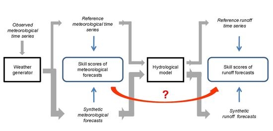
1. Introduction
Numerical runoff predictions are crucial for hydropower and drinking water management e.g., [1,2] as well as for drought preparedness e.g., [3,4]. They are usually produced by forcing a hydrological model with meteorological forecasts or climate projections e.g., [5,6,7]. Runoff predictions are affected by various sources of uncertainty that include, among others, the hydrological model input forcing (such as temperature, precipitation, soil moisture, or snow extent) and the hydrological model structure e.g., [8,9].
This study focuses on how the uncertainty of meteorological forecasts transfer to runoff forecasts. In particular, it investigates how the skill (i.e., quality) of temperature and precipitation forecasts impact on the skill of the resulting runoff forecasts. While the skill of the runoff forecasts in precipitation-driven basins is largely independent from the temperature forecasts e.g., [10], the influence of precipitation and temperature in snow-dominated basins is more nuanced. At lead times up to 10 days, Hay et al. [11] and Clark and Hay [12] found that variations in runoff for snow-dominated basins are more influenced by variations in temperature than by variations in precipitation. Using seasonal forecasts (lead times up to one year) and still referring to snow-dominated basins, Olsson and Lindström [13] highlighted that although temperature has a strong impact in spring, precipitation remains the main forcing with respect to runoff generation. Other studies also showed that the large influence of temperature on the runoff skill in early summer is due to the presence of ice and snow at high altitudes [8,14]. Forecasts covering longer lead times, such as decadal forecasts which aim at lead times up to several years e.g., [15,16], were to our knowledge never used to assess the transfer of skill between meteorological and runoff forecasts.
Future climate projections anticipate virtually unanimously an increase in temperature, and, in general, also an increase in precipitation e.g., [17]. Shrinking snow-covered areas e.g., [1,18,19] and reduced glacier extents e.g., [20,21] are therefore expected. This in turn suggests an increasing importance of precipitation in runoff generation also for snow- and ice-dominated catchments e.g., [22,23,24]. In fact, several studies e.g., [25,26,27,28] showed that with decreasing glacierization, the ice melt contribution to runoff will decrease, while snowmelt and precipitation will increase. In the future, precipitation might thus have a larger impact on runoff than today, and the importance of temperature for runoff formation is therefore expected to decrease accordingly. Although the question of how the forecasts skill of precipitation and temperature reflect into runoff forecasts in snow-dominated basins has been partially investigated e.g., [8,11,12,13,14], it has to our knowledge never assessed with respect to glacierized catchments. In particular, quantitative statements about the relation between the skill of meteorological forecasts and the corresponding runoff predictions are missing.
The objective of this study was threefold: First, to investigate how the forecasts skill of the input meteorological time series is transferred to the runoff predictions over different lead times in glacierized catchments; second, to analyze how the forecasts skill is influenced by the degree of glacierization in a catchment; and third, to evaluate the impact of the hydrological model structure on the results.
2. Methods
2.1. General Methodological Workflow
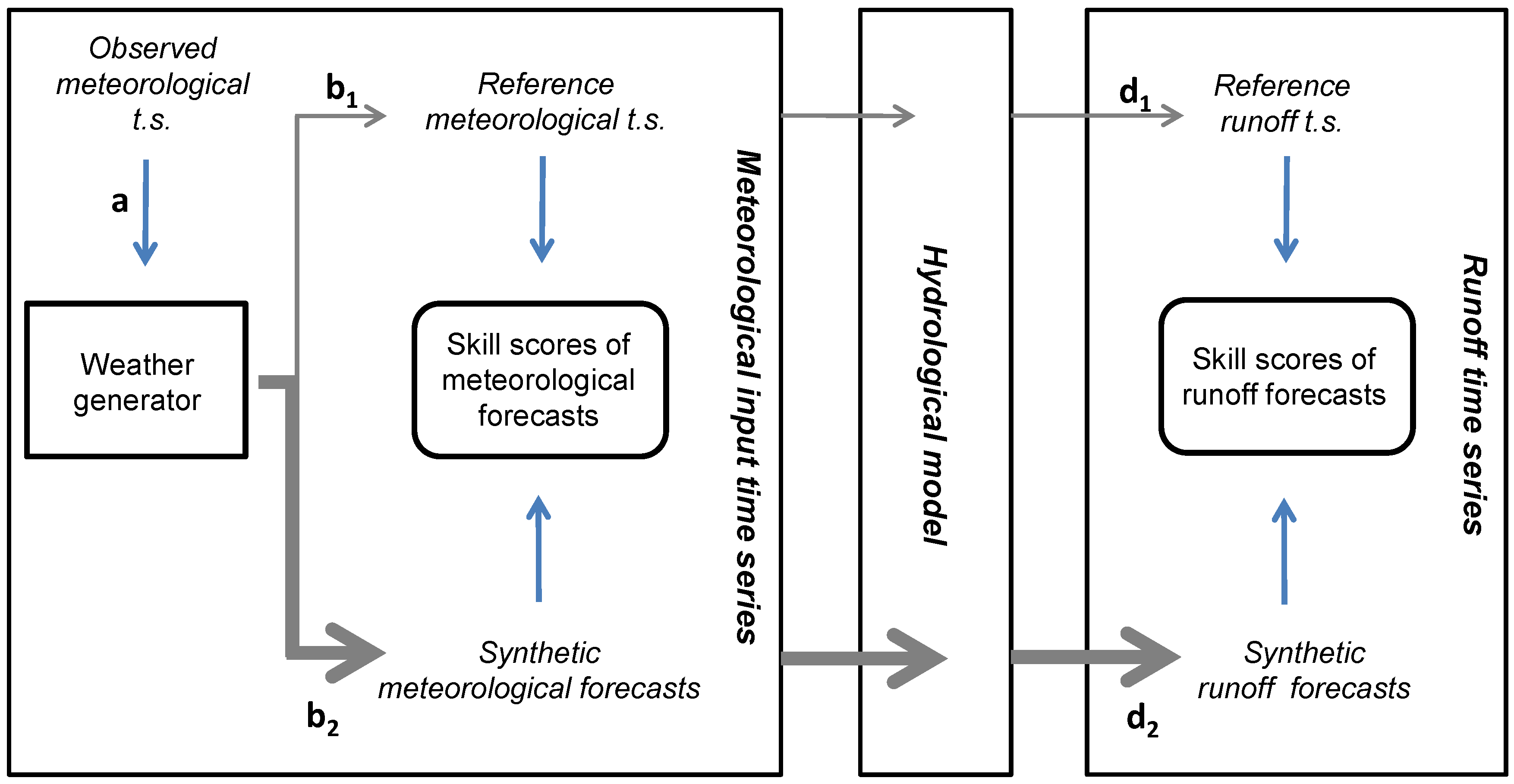
The general methodological workflow of the study is shown in Figure 1. The main elements of the workflow are (i) the meteorological input time series required to drive a hydrological model (Section 2.2); (ii) the hydrological model itself (Section 2.3); and (iii) the resulting runoff time series. Conceptually, we performed all analyses in a virtual world in which the hydrological model is assumed to be prefect. A perfect meteorological input time series thus results in a perfect runoff time series. With this in mind, we used a weather generator to produce a synthetic reference meteorological time series (assumed to be perfect; Section 2.2.1), and superimposed various signals on it to simulate sets of forecasts with varying skill (Section 2.2.2). These synthetic meteorological forecasts were then fed into the same hydrological model, producing a corresponding set of runoff forecasts. The skill of the individual runoff forecasts (Section 2.4) was then computed with respect to the reference runoff time series (the latter is obtained by feeding the reference meteorological time series through the model). The relation by which variations in the skill of the meteorological input propagates to the skill of the hydrological output is the object of our study.
All simulations were performed for two virtual catchments, “A” and “B” (Figure 2), characterized by a glacial hydrological regime. Both catchments have a similar mean air temperature but have a different size, aspect and mean annual precipitation. Individual simulations were performed over several years (decadal time scale) and the degree of glacierization of the two catchments was artificially varied in a set of “Scenarios” (Figure 2) to investigate the glaciers’ role in skill propagation.
2.2. Generation of Synthetic Meteorological Time Series
2.2.1. Reference Meteorological Time Series
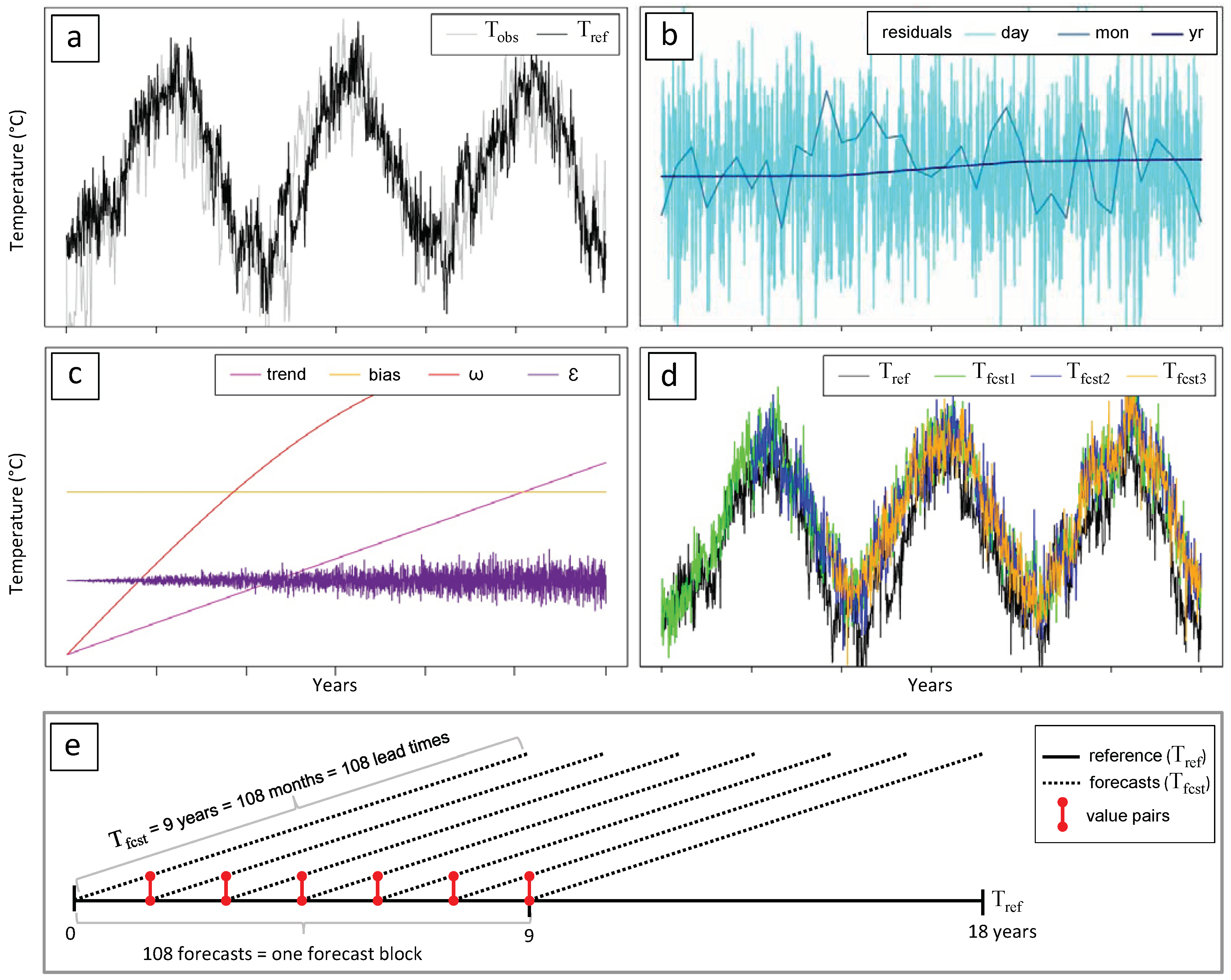
The reference meteorological time series (Figure 1b1), comprising temperature () and precipitation (), were generated with the weather generator described in Farinotti [29]. In a nutshell, the weather generator decomposes a given meteorological time series (Figure 1a) in a long term trend, long term monthly and daily anomalies, and three stochastic variability components capturing (i) year-to-year; (ii) month-to-month; and (iii) day-to-day fluctuations (Figure 3b). The three variability components are characterized by a corresponding set of variability parameters, . For generating synthetic time series, the weather generator uses a sequence of Auto-Regressive Moving-Average (ARMA) models. In the case of precipitation, a Markov chain model is additionally employed to produce realistic sequences of wet and dry days.
To estimate the variability parameters required to produce the synthetic reference time series for Catchments A and B, the weather generator was trained on real-world meteorological observations used in Farinotti et al. [28] (example for temperature, Figure 3a). The weather generator was then used to produce a reference time series with an arbitrary length of 18 years. The time series had daily resolution, which is the resolution at which all our simulations are performed. For additional details on the weather generator, refer to Farinotti [29].
2.2.2. Synthetic Meteorological Forecasts
The synthetic meteorological forecasts ( and ; Figure 1b2) were created by (a) using the weather generator described above to produce sets of additional meteorological time series with different variability, and (b) superimposing several components – namely a trend, a bias, a long-term oscillation (i.e., a signal varying over several decades) and random noise – to them (Figure 3).
More specifically: Let and be the temperature and precipitation generated with the weather generator (WG) for a given point in time t and a given set of variability parameter . Let, moreover, be the time period over which the synthetic forecasts are generated. and were then given by:
where a is the trend magnitude at , b is a bias, is a long-term oscillation of the form
and are noise terms (see below). In the long-term oscillation, c is the amplitude. Note also that the periodicity is much longer than our forecast period, which aims at representing long-term natural variability. For the noise term, we chose the arbitrary form
where is a random realization of a normal distribution with with mean ( and in our case) and standard deviation . In the equation, parameters and can be interpreted as the noise level at the beginning () and the end () of the forecast, respectively. We choose , which means that there is no noise at the beginning of the forecast, and , which means that the noise intensity increases with forecasting lead time. The form of the various components added to the time series obtained from the weather generator are shown in Figure 3c.
It is important to note that the exact form of the elements in Equations (1)–(4) is not of further importance, since precisely reproducing the structure of deviations in real-world forecasts was outside the scope of the study. Rather, we aimed at obtaining a set of individual forecasts with a wide range of skills: From very good ones close to the reference time series, to very poor ones close to arbitrary noise.
For a given set of parameters (), we created forecasts that start every months during 9 years. This makes a total of forecasts per parameter set (Figure 3d,e). We call such a set of 108 forecasts a “forecast block”. The length of the synthetic forecasts was also 9 years (in the above notation: yr). With this, every forecasts could be validated against the reference meteorological time series over a period of 9 years.
To imitate a variety of possible forecast, we varied parameters and over three levels (Table 1). The parameter values were chosen arbitrarily. Out of the possible combinations, and due to computational limitations, we then selected a random subset of 150 realizations for further analyses.
2.3. Runoff Forecasts Generation
The reference meteorological time series (Section 2.2.1) and the synthetic forecasts (Section 2.2.2) were fed into two hydrological models (see below) to obtain corresponding reference runoff time series (Figure 1d1) and runoff forecasts (Figure 1d2). For every simulation, the hydrological models were initialized with a one-year spin-up phase driven by the reference meteorological time series. To isolate the impact of glacierization on the skill transfer, both models were run with five different scenarios for glacier extents and ice volumes (Table 2, Figure 2).
The two hydrological models were the Glacier Evolution Runoff Model (GERM) and the Hydrologiska Byråns Vattenbalansavdelning-light (HBV-light). GERM [26,28] is a fully distributed, deterministic model simulating catchment runoff at daily time scales. The model includes different modules for snow accumulation, snow and ice ablation, glacier evolution, evapotranspiration, and runoff routing. It requires continuous temperature and precipitation time series as input, a digital surface model of the catchment, as well as the glacier ice thickness distribution. To simulate glacier evolution, the model implements the so-called -parametrization [30], which is a simple mass conserving approach based on the observation that the largest changes in ice thickness occur at the glacier tongue. HBV-light [31] is a semi-distributed conceptual model constituted of four different routines, namely a snow and glacier routine, a soil moisture routine, a response routine, and a runoff routine. For representing the glaciers, the new “Glacier Area Change Routine” presented in Seibert et al. [32] was used. The latter is based on the -parametrization as well. The required input data for HBV-light, including the glacier routine, are continuous daily temperature and precipitation, monthly mean temperatures and mean potential evapotranspiration, as well as information about the glacier thickness per elevation band. For more details on the HBV-light model, refer to Seibert [33] and Seibert and Vis [31].
2.4. Skill Scores
The performance of the various forecasts (, , ) was quantified with two different and complementary skill scores: The Root Mean Square Error (RMSE, Equation (5)) and the Nash-Sutcliffe efficiency coefficient (NSE, Equation (6)). Let and be the reference and forecasted values of a given variable X and lead time i, respectively. RMSE and NSE are then given by:
where N is the number of data pairs ( in our case, see below), and is the variance of . In the above equations, X can either be temperature (T), precipitation (P) or runoff (Q). In the following, we denote the skill scores (RMSE or NSE) for the temperature, precipitation and runoff forecasts with , and respectively.
RMSE measures the average magnitude of the deviation between reference and forecast time series. NSE, instead, measures the deviation relative to the variability in the reference time series. RMSE values range between 0 (best score) and ∞, and the ones of NSE between and 1 (best score).
In our analyses, all skill scores were evaluated by aggregating the individual time series to monthly values. Since all forecasts were 9 years in length, skill scores were computed for lead times. Similarly, since the forecasts were started every months over 9 years, the score of each of the 108 lead times was computed from value pairs (Figure 3e).
3. Results and Discussion
The results generated by forcing the two different hydrological models (GERM and HBV) with the 150 forecast blocks are presented hereafter. We first address the influence of lead time on the results (Section 3.1) and assess the skill transfer between meteorological and runoff forecasts afterwards (Section 3.2).
3.1. Dependence on Lead Time
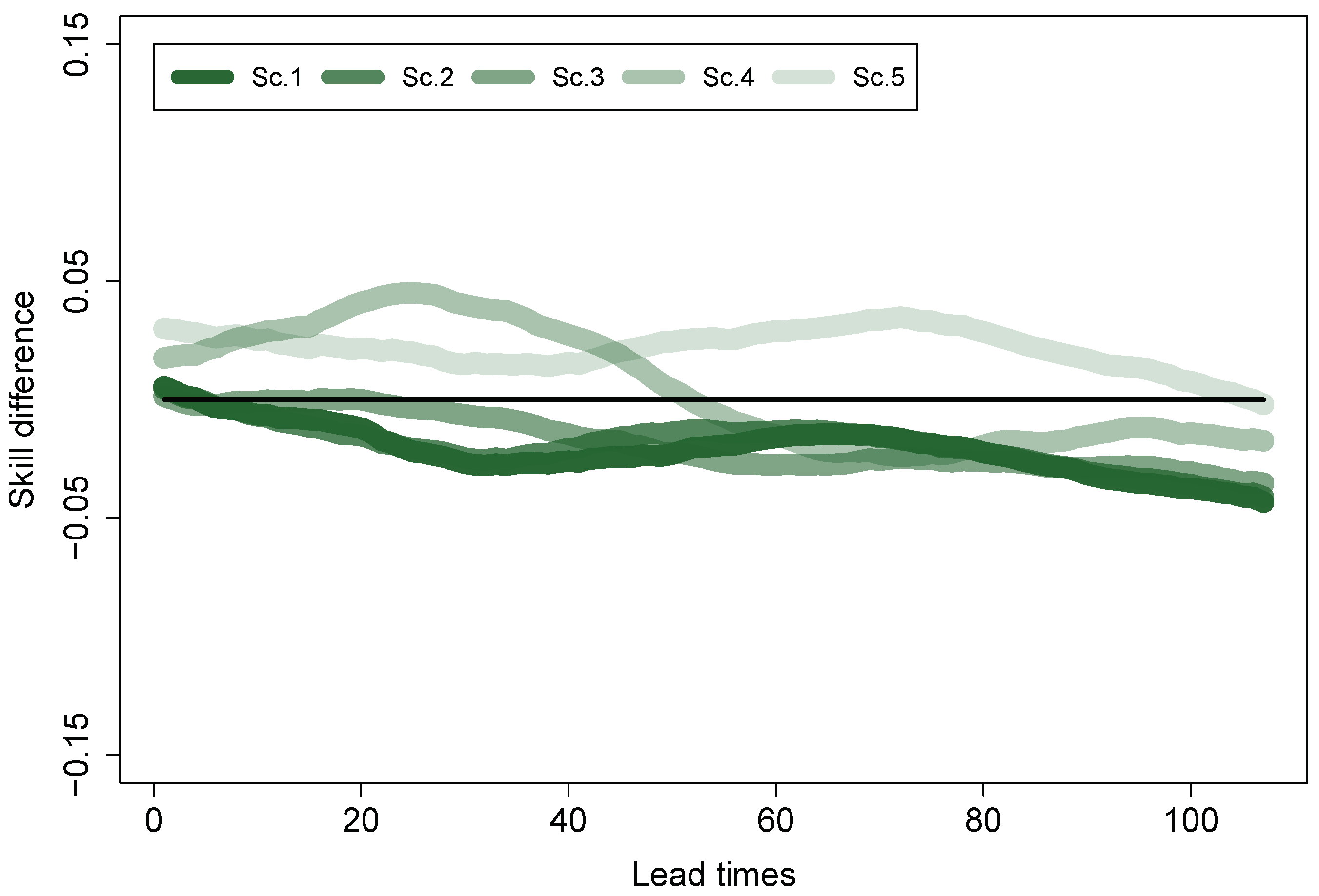
The skill scores for runoff (), temperature (), and precipitation () were transformed as to have different units. To allow for intercomparison between them, we first normalized the values obtained for every lead time separately (this means that, for every lead time, the three variables have values ranging between 0 and 1). Figure 4 presents the difference between the skill in the meteorological forecasts (average over and ) and the skill in the resulting runoff predictions () for different lead times. This difference remains approximately constant over the lead times, despite the fact that the skill of both precipitation and temperature decreases with increasing lead time. This indicates that all further observations—and the inter-relations between , , and in particular—are independent from the lead time. Loosely speaking, this means that the combination of a good temperature forecast and a good precipitation forecast result in a good runoff forecast, while the combination of a poor temperature forecast and a poor precipitation forecast result in a poor runoff forecast, rather than in a disastrous one. This result also indicates that the skill in temperature and precipitation forecasts is interchangeable at every lead time, i.e., that a poor skill in precipitation forecasts can be compensated by a good skill in the temperature forecasts, and vice-versa.
3.2. Skill Transfer between Meteorological and Runoff Forecasts
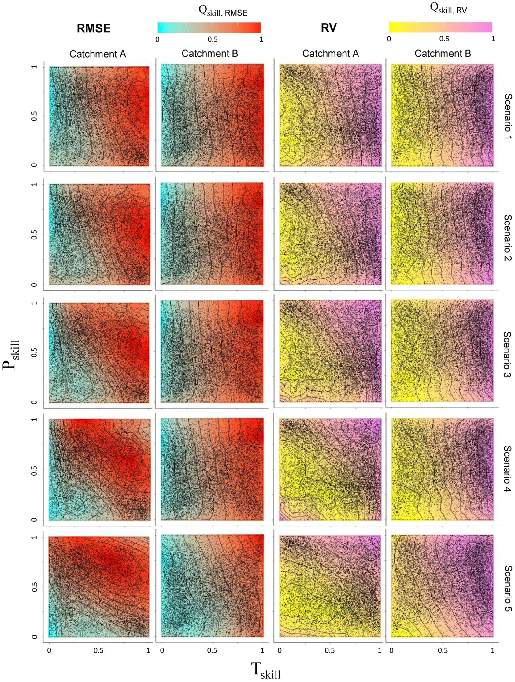
The relationship between , and from the 150 forecast blocks is shown in Figure 5. Since the dependence on lead time was assessed to be of minor relevance (Section 3.1), a mean value over all lead times is calculated for each forecast block. We observe that for Scenario 1 (highest glacierization), the relationship between and is stronger (more pronounced horizontal color variations in Figure 5) than and . The observation holds true in both catchments, and is more visible in Catchment B than in Catchment A. With decreasing glacierization (Scenarios 2 to 5) the horizontal color gradient shifts towards a vertical gradient, suggesting an increasing influence of (and decreasing influence of ) on . This shift is more pronounced in Catchment A than Catchment B.
In order to quantify the relationship between the meteorological and the runoff forecasts (i.e., the transfer of forecast skill), we express as a linear function of and :
In the above equation, parameters m and n are determined by ordinary least-square regression, and is the residual of the relation. The values of m and n can be interpreted as the strength by which the runoff forecasts are influenced by the temperature and precipitation forecasts, respectively. The mean values of m and n (mean over all lead times), along with the mean coefficient of determination , are given in Table 3.
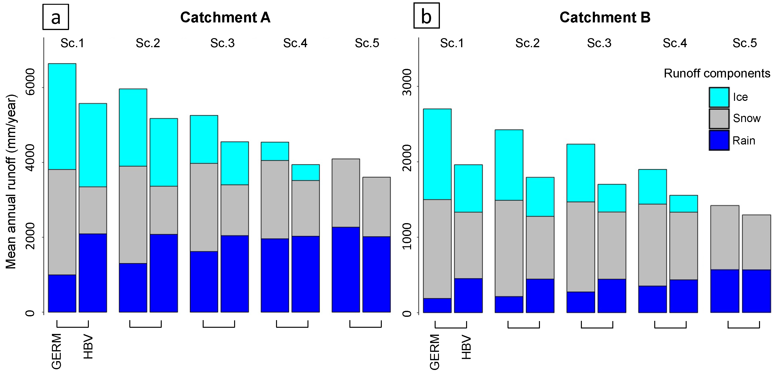
For Scenario 1 and RMSE, we found and for Catchment A, and and for Catchment B. This indicates that has a larger impact on the resulting than has (an equivalent result is found when considering NSE; cf. Table 1). This result matches our hypothesis that, in glacierized catchments, temperature has a larger influence on runoff compared to precipitation, which we interpret as a result of the direct impact of temperature on snow and ice melt, and thus runoff generation. In general, we observe that has a larger influence on than has (values of m four times the values of n, on average), and that the difference between m and n is larger in Catchment B than it is in Catchment A. This indicates that is more strongly influenced by the skill of the temperature forecasts than it is by the precipitation forecasts, especially in Catchment B. We suggest this to be related to the larger amount of runoff that originates from snow and ice melt in Catchment B compared to A (Figure 6). Note that due to the higher fraction of catchment area lying below the equilibrium line in the case of Catchment B, the runoff share from snow and ice melt is larger than in Catchment A despite the lower glacierization (Figure 2). With decreasing glacierization (from Scenario 1 to Scenario 5), the values of parameter m decrease, while the ones of n increase. This is true for both the considered skill scores (Table 3) and means that the impact of on diminished with shrinking ice extent, while increases its influence. Again, the diminishing amount of ice and snow melt, and the increasing one of precipitation, can explain this trend (Figure 6).
For Catchment A, the influence of is stronger than the one of for glacierizations below 30% (solid lines in Figure 7a). In Catchment B, however, continues to have a stronger influence on even if there is no glacier left. We suggest this to be linked to the fact that in Catchment B the runoff share originating from ice and snow melt (sum of both components) is higher than the one originating from liquid precipitation, even in a scenario without glacier (Figure 6b, Scenario 5). This makes the catchment’s runoff more sensitive to temperature than for Catchment A, in which the proportion of ice and snow melt is lower (Figure 6a). Figure 7b suggests that temperature will have the larger impact on runoff compared to precipitation if the sum of the ice and snow melt contributions is higher than about 60%.
The above results are similar for both hydrological models (Figure 7c,d). The small differences could be related to the different runoff composition predicted by two models (Figure 6). For the same meteorological input time series, for example, the amount of runoff produced by HBV is lower than the one produced by the GERM model. We interpret this as an indication for the HBV model storing more water in one or several storage compartments (such as the snowpack or the soil) than GERM.
4. Conclusions
This study investigated the transfer of skill between meteorological and runoff forecasts. Synthetic meteorological forecasts for which the skill was manually controlled were generated, and fed into two separate hydrological models. Five scenarios representing different glacier ice volumes and ice extents were tested to assess the influence of glacierization on the results. The relation between the skill of the meteorological forecasts and runoff predictions was quantified through linear regression, and through a series of dedicated analyses.
For high degrees of glacierization (>50%), temperature showed an impact on runoff up to four times larger than precipitation, which we interpret as an expression of the temperature’s control on both ice and snow melt. With shrinking glaciers and smaller glacierization, the influence of temperature decreased steadily, while the opposite was true for precipitation. For the two investigated catchments, temperature maintained a larger control on runoff compared to precipitations if the glacierizations was above 30%, or if the ice- and snow-melt contribution to total runoff was more than ca. 60%. The two hydrological models gave similar results, and the relations were shown to hold true independently of the lead time considered.
Our results are of relevance for the application of new generations of long- and extended-range meteorological forecasts—including decadal predictions—as those have been shown to be more skillful in predicting temperature than precipitation e.g., [34,35,36]. In particular, we suggest that using such type of predictions to produce runoff forecasts in snow- and glacier-dominated catchments holds more promise than doing so in catchments dominated by liquid precipitation.
Author Contributions
Both authors conceived and designed the experiments, and analyzed the results; S.G. performed the experiments, analysed the data and wrote the manuscript with contributions from D.F.
Funding
This study was funded by the Swiss National Science Foundation (SNSF) grant number PZENP2_154290.
Acknowledgments
We thank Davide Sauerwein for the help in producing the HBV simulations and Manuela Brunner for commenting an earlier version of the manuscript. The critical comments of the editor Christophe Kinnard are acknowledged.
Conflicts of Interest
The authors declare no conflict of interest.
References
- Barnett, T.P.; Adam, J.C.; Lettenmaier, D.P. Potential impacts of a warming climate on water availability in snow-dominated regions. Nature 2005, 438, 303–309. [Google Scholar] [CrossRef] [PubMed]
- Chandramowli, S.N.; Felder, F.A. Impact of climate change on electricity systems and markets—A review of models and forecasts. Sustain. Energy Technol. Assess. 2014, 5, 62–74. [Google Scholar] [CrossRef]
- Panu, U.S.; Sharma, T.C. Challenges in drought research: some perspectives and future directions. Hydrol. Sci. J. 2002, 47, S19–S30. [Google Scholar] [CrossRef]
- Wilhite, D.A.; Knutson, C.L. Drought management planning: Conditions for success. Opt. Mediterr. Ser. A 2008, 80, 141–148. [Google Scholar]
- Zappa, M.; Rotach, M.W.; Arpagaus, M.; Dorninger, M.; Hegg, C.; Montani, A.; Ranzi, R.; Ament, F.; Germann, U.; Grossi, G.; et al. MAP D-PHASE: Real-time demonstration of hydrological ensemble prediction systems. Atmos. Sci. Lett. 2008, 9, 80–87. [Google Scholar] [CrossRef]
- Liechti, K.; Zappa, M.; Fundel, F.; Germann, U. Probabilistic evaluation of ensemble discharge nowcasts in two nested Alpine basins prone to flash floods: Evaluation of Ensemble Discharge Nowcast In Two Nested Alpine Basins. Hydrol. Proc. 2013, 27, 5–17. [Google Scholar] [CrossRef]
- Hidalgo-Muñoz, J.M.; Gámiz-Fortis, S.R.; Castro-Díez, Y.; Argüeso, D.; Esteban-Parra, M.J. Long-range seasonal streamflow forecasting over the Iberian Peninsula using large-scale atmospheric and oceanic information. Water Resour. Res. 2015, 51, 3543–3567. [Google Scholar] [CrossRef]
- Wood, A.W.; Lettenmaier, D.P. An ensemble approach for attribution of hydrologic prediction uncertainty. Geophys. Res. Lett. 2008, 35, 1–5. [Google Scholar] [CrossRef]
- Shukla, S.; Sheffield, J.; Wood, E.F.; Lettenmaier, D.P. On the sources of global land surface hydrologic predictability. Hydrol. Earth Syst. Sci. 2013, 17, 2781–2796. [Google Scholar] [CrossRef]
- Crochemore, L.; Ramos, M.H.; Pappenberger, F. Bias correcting precipitation forecasts to improve the skill of seasonal streamflow forecasts. Hydrol. Earth Syst. Sci. 2016, 20, 3601–3618. [Google Scholar] [CrossRef]
- Hay, L.E.; Clark, M.P.; Wilby, R.L.; Gutowski, W.J., Jr.; Leavesley, G.H.; Pan, Z.; Arritt, R.W.; Takle, E.S. Use of regional climate model output for hydrologic simulations. J. Hydrometeorol. 2002, 3, 571–590. [Google Scholar] [CrossRef]
- Clark, M.P.; Hay, L.E. Use of medium-range numerical weather prediction model output to produce forecasts of streamflow. J. Hydrometeorol. 2004, 5, 15–32. [Google Scholar] [CrossRef]
- Olsson, J.; Lindström, G. Evaluation and calibration of operational hydrological ensemble forecasts in Sweden. J. Hydrol. 2008, 350, 14–24. [Google Scholar] [CrossRef]
- Yossef, N.C.; Winsemius, H.; Weerts, A.; van Beek, R.; Bierkens, M.F.P. Skill of a global seasonal streamflow forecasting system, relative roles of initial conditions and meteorological forcing: Skill of a Global Seasonal Streamflow Forecasting System. Water Resour. Res. 2013, 49, 4687–4699. [Google Scholar] [CrossRef]
- Meehl, G.A.; Goddard, L.; Murphy, J.; Stouffer, R.J.; Boer, G.; Danabasoglu, G.; Dixon, K.; Giorgetta, M.A.; Greene, A.M.; Hawkins, E.; et al. Decadal Prediction: Can It Be Skillful? Bull. Am. Meteorol. Soc. 2009, 90, 1467–1485. [Google Scholar] [CrossRef]
- Cane, M.A. Climate science: Decadal predictions in demand. Nat. Geosci. 2010, 3, 231–232. [Google Scholar] [CrossRef]
- Solomon, S. (Ed.) Climate Change 2013—The Physical Science Basis: Working Group I Contribution to the Fifth Assessment Report of the Intergovernmental Panel on Climate Change; Cambridge University Press: Cambridge, UK, 2014. [Google Scholar]
- Bavay, M.; Grünewald, T.; Lehning, M. Response of snow cover and runoff to climate change in high Alpine catchments of Eastern Switzerland. Adv. Water Resour. 2013, 55, 4–16. [Google Scholar] [CrossRef]
- Marty, C.; Schlögl, S.; Bavay, M.; Lehning, M. How much can we save? Impact of different emission scenarios on future snow cover in the Alps. Cryosphere 2017, 11, 517–529. [Google Scholar] [CrossRef]
- Farinotti, D.; Longuevergne, L.; Moholdt, G.; Duethmann, D.; Mölg, T.; Bolch, T.; Vorogushyn, S.; Güntner, A. Substantial glacier mass loss in the Tien Shan over the past 50 years. Nat. Geosci. 2015, 8, 716–722. [Google Scholar] [CrossRef]
- Huss, M.; Hock, R. A new model for global glacier change and sea-level rise. Front. Earth Sci. 2015, 3, 54. [Google Scholar] [CrossRef]
- Hock, R.; Jansson, P.; Braun, L.N. Modelling the response of mountain glacier discharge to climate warming. In Global Change and Mountain Regions; Springer: Berlin/Heidelberg, Germany, 2005; pp. 243–252. [Google Scholar]
- Stahl, K.; Moore, R.D.; Shea, J.M.; Hutchinson, D.; Cannon, A.J. Coupled modelling of glacier and streamflow response to future climate scenarios: Modeling of glacier and streamflow. Water Resour. Res. 2008, 44, 1–13. [Google Scholar] [CrossRef]
- Ragettli, S.; Pellicciotti, F.; Bordoy, R.; Immerzeel, W.W. Sources of uncertainty in modeling the glaciohydrological response of a Karakoram watershed to climate change: Sources of uncertainty in glaciohydrological modeling. Water Resour. Res. 2013, 49, 6048–6066. [Google Scholar] [CrossRef]
- Singh, P.; Kumar, N. Impact assessment of climate change on the hydrological response of a snow and glacier melt runoff dominated Himalayan river. J. Hydrol. 1997, 193, 316–350. [Google Scholar] [CrossRef]
- Huss, M.; Farinotti, D.; Bauder, A.; Funk, M. Modelling runoff from highly glacierized alpine drainage basins in a changing climate. Hydrol. Proc. 2008, 22, 3888–3902. [Google Scholar] [CrossRef]
- Weber, M.; Braun, L.; Mauser, W.; Prasch, M. Contribution of rain, snow-and icemelt in the Upper Danube discharge today and in the future. Geogr. Fis. Din. Quat. 2010, 33, 221–230. [Google Scholar]
- Farinotti, D.; Usselmann, S.; Huss, M.; Bauder, A.; Funk, M. Runoff evolution in the Swiss Alps: Projections for selected high-alpine catchments based on ENSEMBLES scenarios. Hydrol. Proc. 2012, 26, 1909–1924. [Google Scholar] [CrossRef]
- Farinotti, D. On the effect of short-term climate variability on mountain glaciers: Insights from a case study. J. Glaciol. 2013, 59, 992–1006. [Google Scholar] [CrossRef]
- Huss, M.; Jouvet, G.; Farinotti, D.; Bauder, A. Future high-mountain hydrology: A new parameterization of glacier retreat. Hydrol. Earth Syst. Sci. 2010, 14, 815–829. [Google Scholar] [CrossRef]
- Seibert, J.; Vis, M.J.P. Teaching hydrological modeling with a user-friendly catchment-runoff-model software package. Hydrol. Earth Syst. Sci. 2012, 16, 3315–3325. [Google Scholar] [CrossRef] [Green Version]
- Seibert, J.; Vis, M.J.P.; Kohn, I.; Weiler, M.; Stahl, K. Technical note: Representing glacier geometry changes in a semi-distributed hydrological model. Hydrol. Earth Syst. Sci. 2018, 22, 2211–2224. [Google Scholar] [CrossRef]
- Seibert, J. HBV light. In User’s Manual; Uppsala University: Uppsala, Sweden, 1996. [Google Scholar]
- Meehl, G.A.; Goddard, L.; Boer, G.; Burgman, R.; Branstator, G.; Cassou, C.; Corti, S.; Danabasoglu, G.; Doblas-Reyes, F.; Hawkins, E. Decadal climate prediction: an update from the trenches. Bull. Am. Meteorol. Soc. 2014, 95, 243–267. [Google Scholar] [CrossRef]
- Scaife, A.A.; Athanassiadou, M.; Andrews, M.; Arribas, A.; Baldwin, M.; Dunstone, N.; Knight, J.; MacLachlan, C.; Manzini, E.; Müller, W.A.; et al. Predictability of the quasi-biennial oscillation and its northern winter teleconnection on seasonal to decadal timescales. Geophys. Res. Lett. 2014, 41, 1752–1758. [Google Scholar] [CrossRef] [Green Version]
- Jia, L.; Yang, X.; Vecchi, G.A.; Gudgel, R.G.; Delworth, T.L.; Rosati, A.; Stern, W.F.; Wittenberg, A.T.; Krishnamurthy, L.; Zhang, S.; et al. Improved Seasonal Prediction of Temperature and Precipitation over Land in a High-Resolution GFDL Climate Model. J. Clim. 2015, 28, 2044–2062. [Google Scholar] [CrossRef]
Figure 1.
General methodological workflow. The three boxes represent the different working steps. The thin grey arrows are the reference time series (t.s.) while the thick grey ones are different synthetic forecasts. Blue arrows indicate input data.
Figure 1.
General methodological workflow. The three boxes represent the different working steps. The thin grey arrows are the reference time series (t.s.) while the thick grey ones are different synthetic forecasts. Blue arrows indicate input data.

Figure 2.
Overview map of the two synthetic catchments A and B. The surface types characterizing the catchments are given by different colors. Glaciers are in white and the colored outlines depict the ice extents used for different model runs (Scenarios 1–5, see Section 2.3 and Table 2). Scenario 5 simulates runoff in an ice-free catchment.

Figure 3.
Methodology used to produce the synthetic weather forecasts. (a) Observed temperature time series () and reference time series produced with the weather generator (). (b) Decomposition of the residuals of in a daily, monthly and yearly variability. (c) Trend, bias, oscillation () and noise () added to to generate the (d) synthetic forecasts (). (e) Illustration of a forecast block composed of 108 forecasts of 9 years in length, as well as the value pairs used to calculate the skill scores (Section 2.4). The values pairs are shown for lead time 1, meaning that the values of the meteorological forecasts and the ones of the reference time series are paired after one month. The scales in the figure are arbitrary and are meant for illustration purposes only.

Figure 4.
Skill difference between meteorological and runoff forecasts over all lead times. Individual lines refer to the scenarios (Sc.) defined in Table 2 and are means over the two catchments.
Figure 4.
Skill difference between meteorological and runoff forecasts over all lead times. Individual lines refer to the scenarios (Sc.) defined in Table 2 and are means over the two catchments.

Figure 5.
Relation between temperature, precipitation and runoff skill scores (, , and ) for the two catchments (A and B), both skill scores (RMSE and NSE) and all Scenarios. The individual panels show the and calculated for all forecast blocks and lead times (150 blocks with · 108 lead times each, resulting in 16,000 combinations (black dots)), together with the mean (colors). The runoff skill scores were interpolated with a local quadratic trend surface. All results refer to the GERM model.

Figure 6.
Runoff originating from ice melt, snow melt and liquid precipitation for the five scenarios in Catchment A (a) and Catchment B (b). Values refer to the scenarios given in Table 2 and were calculated by forcing the two hydrological models (GERM and HBV) with the reference meteorological time series.

Figure 7.
Mean values (mean over all lead times) of parameters m and n (cf. Equation (7)), and their relation to (a + c) glacierization and (b + d) the sum of ice and snow melt. Panels (a) + (b) and (c) + (d) refer to the GERM and HBV model, respectively. Results refer to the RMSE skill score.
Figure 7.
Mean values (mean over all lead times) of parameters m and n (cf. Equation (7)), and their relation to (a + c) glacierization and (b + d) the sum of ice and snow melt. Panels (a) + (b) and (c) + (d) refer to the GERM and HBV model, respectively. Results refer to the RMSE skill score.


Table 1.
Parameters used to create the synthetic temperature and precipitation forecasts (see Equations (1) and (2) for details). Note that the values for are given relative to the ones used to produce the synthetic reference time series (a value of, e.g., “2” means that , , were doubled).
| Parameter | Forecast | ||
|---|---|---|---|
| Temperature | Precipitation | ||
| variability (relative) | |||
| a | trend | (C) | (%) |
| b | bias | (C) | (%) |
| c | oscillation amplitude | (C) | (%) |
| mean of the noise term | 0 | 1 | |
| noise level at | 0 | 0 | |
| noise level at | |||
Table 2.
Glacierization (glac.) and glacier ice volume () in each scenario. Scenario 1 has the largest glacier volume and Scenario 5 has no glacier left. The spatial extent of the glaciers is shown in Figure 2.
Table 2.
Glacierization (glac.) and glacier ice volume () in each scenario. Scenario 1 has the largest glacier volume and Scenario 5 has no glacier left. The spatial extent of the glaciers is shown in Figure 2.
| Scenario | Catchment A | Catchment B | ||
|---|---|---|---|---|
| glac. (%) | (km) | glac. (%) | (km) | |
| Scenario 1 | 61.02 | 0.43 | 53.56 | 1.29 |
| Scenario 2 | 49.70 | 0.29 | 49.56 | 0.99 |
| Scenario 3 | 32.38 | 0.17 | 36.03 | 0.58 |
| Scenario 4 | 15.63 | 0.06 | 24.19 | 0.36 |
| Scenario 5 | 0.00 | 0.00 | 0.00 | 0.00 |
Table 3.
Parameters m and n and corresponding coefficient of determination () of Equation (7) for the two analyzed catchments and both skill scores. Results refer to the GERM model.
Table 3.
Parameters m and n and corresponding coefficient of determination () of Equation (7) for the two analyzed catchments and both skill scores. Results refer to the GERM model.
| Catchment A | Catchment B | |||||||||||
|---|---|---|---|---|---|---|---|---|---|---|---|---|
| RMSE | NSE | RMSE | NSE | |||||||||
| Scenario 1 | 0.69 | 0.71 | 0.75 | 0.26 | 0.28 | 0.73 | 0.75 | 0.72 | 0.73 | 0.14 | 0.15 | 0.68 |
| Scenario 2 | 0.60 | 0.62 | 0.69 | 0.33 | 0.34 | 0.67 | 0.75 | 0.70 | 0.74 | 0.10 | 0.10 | 0.68 |
| Scenario 3 | 0.50 | 0.52 | 0.64 | 0.40 | 0.42 | 0.62 | 0.66 | 0.59 | 0.72 | 0.17 | 0.18 | 0.65 |
| Scenario 4 | 0.38 | 0.39 | 0.58 | 0.46 | 0.48 | 0.57 | 0.56 | 0.50 | 0.68 | 0.19 | 0.20 | 0.60 |
| Scenario 5 | 0.26 | 0.25 | 0.58 | 0.54 | 0.55 | 0.55 | 0.43 | 0.36 | 0.58 | 0.25 | 0.23 | 0.50 |
© 2018 by the authors. Licensee MDPI, Basel, Switzerland. This article is an open access article distributed under the terms and conditions of the Creative Commons Attribution (CC BY) license (http://creativecommons.org/licenses/by/4.0/).
Share and Cite
MDPI and ACS Style
Gindraux, S.; Farinotti, D. Skill Transfer from Meteorological to Runoff Forecasts in Glacierized Catchments. Hydrology 2018, 5, 26. https://doi.org/10.3390/hydrology5020026
AMA Style
Gindraux S, Farinotti D. Skill Transfer from Meteorological to Runoff Forecasts in Glacierized Catchments. Hydrology. 2018; 5(2):26. https://doi.org/10.3390/hydrology5020026
Chicago/Turabian StyleGindraux, Saskia, and Daniel Farinotti. 2018. "Skill Transfer from Meteorological to Runoff Forecasts in Glacierized Catchments" Hydrology 5, no. 2: 26. https://doi.org/10.3390/hydrology5020026
Note that from the first issue of 2016, this journal uses article numbers instead of page numbers. See further details here.