Article

Hydrologic Characteristics of Streamflow in the Southeast Atlantic and Gulf Coast Hydrologic Region during 1939–2016 and Conceptual Map of Potential Impacts

1
Biological Systems Engineering, College of Agriculture and Food Sciences, Florida A&M University, Tallahassee, FL 32307, USA
2
School of the Environment, Florida A&M University, Tallahassee, FL 32307, USA
3
College of Agriculture and Food Sciences, Florida A&M University, Tallahassee, FL 32307, USA
*
Author to whom correspondence should be addressed.
Hydrology 2018, 5(3), 42; https://doi.org/10.3390/hydrology5030042
Submission received: 2 January 2018 / Revised: 17 June 2018 / Accepted: 30 June 2018 / Published: 7 August 2018
(This article belongs to the Special Issue Climatic Change Impact on Hydrology)

Abstract

:
Streamflow is one the most important variables controlling and maintaining aquatic ecosystem integrity, diversity, and sustainability. This study identified and quantified changes in 34 hydrologic characteristics and parameters at 30 long term (1939–2016) discharge stations in the Southeast Atlantic and Gulf Coast Hydrologic Region (Region 3) using Indicators of Hydrologic Alteration (IHA) variables. The southeastern United States (SEUS) is a biodiversity hotspot, and the region has experienced a number of rapid land use/land cover changes with multiple primary drivers. Studies in the SEUS have been mostly localized on specific rivers, reservoir catchments and/or species, but the overall region has not been assessed for the long-term period of 1939–2016 for multiple hydrologic characteristic parameters. The objectives of the study were to provide an overview of multiple river basins and 31 hydrologic characteristic parameters of streamflow in Region 3 for a longer period and to develop a conceptual map of impacts of selected stressors and changes in hydrology and climate in the SEUS. A seven step procedure was used to accomplish these objectively: Step 1: Download data from the 30 USGS gauging stations. Steps 2 and 3: Select and analyze the 31 IHA parameters using boxplots, scatter plots, and PDFs. Steps 4 and 5: Synthesize the drivers of changes and alterations and the various change points in streamflow in the literature. Step 6: Synthesize the climate of the SEUS in terms of temperature and precipitation changes. Step 7: Develop a conceptual map of impacts of selected stressors on hydrology using Driver–Pressure–State-Impact–Response (DPSIR) framework and IHA parameters. The 31 IHA parameters were analyzed. The meta-analysis of literature in the SEUS revealed the precipitation changes observed ranged from −30% to +35% and temperature changes from −2 °C to 6 °C by 2099. The fiftieth percentile of the Global Climate Models (GCM) predict no precipitation change and an increase in the temperature of 2.5 °C in the region by 2099. Among the GCMs, the 5th and 95th percentile of precipitation changes range between −40% and 110% and temperature changes between −2 °C and 6 °C by 2099. Meta-analysis of land use/land cover show the region has experienced changes. A number of rapid land use/land cover changes in 1957, 1970, and 1998 are some of the change points documented in the literature for precipitation and streamflow in the region. A conceptual map was developed to represent the impacts of selected drivers and the changes in hydrology and climate in the study region for three land use/land cover categories in three different periods.

1. Introduction

Streamflow has been called the “master variable” or the “maestro…that orchestrates pattern and process in rivers” [1]. Streamflow controls and maintains the function, structure, and dynamics of aquatic ecosystems in riparian zones, including flood plains and adjacent wetlands. The magnitude, timing, and duration of typical hydrologic flow characteristics and events, such as monthly median flows and annual low flow events, provide the necessary stable and expected conditions for aquatic life. Organisms require predictable patterns in magnitude, timing, frequency, duration, and extremes of flow events each year, decade, century, and millennium for their continued success and survival. The streamflow, which formerly provided a range of habitats (e.g., stream channel, flood plain, alluvial aquifer, and hyporheic zone), no longer provides the range of hydrologic events that it once did [1,2] due to multiple stressors.
The southeastern United States (SEUS) is a biodiversity hotspot [3] with the highest overall native richness of any temperate region in North America [4]. The region is considered the “wood basket” of the United States (US), producing about half of the country’s timber supply, and is one of the major agricultural areas in the nation [5,6]. The SEUS struggles with water related conflicts [7]. Dams were constructed on many of the free-flowing rivers in the SEUS for flood relief, power generation purposes, and, in some cases, water supply (Atlanta). These modifications were further exacerbated by additional stressors over the last century in the region, such as urbanization, land cover and population change, warming temperatures, and increases in annual precipitation [7]. These have important implications on the region’s biodiversity, ecosystem sustainability, and integrity [8].
The SEUS has been underrepresented in hydroclimatic research [7]. Studies in this region have been primarily focused on specific rivers, reservoir catchments, and/or species [9,10], but the overall region has not been assessed. Most of these studies focus on shorter periods; fewer stations [7,11]; and fewer hydrologic characteristic parameters, such as floods [9], droughts, and average flows. Very few studies have used multiple hydrologic characteristic parameters (e.g., the Indicators of Hydrologic Alteration (IHA) program for smaller regions) [12]. The details of several studies in the different regions in the SEUS are provided in Table S1 in the Supplementary Materials.
Our study attempted to fill in some of these lacunae in research. The specific objectives of the study were: (1) to provide an overview of the multiple hydrologic characteristic parameters of streamflow in the region for a longer period and in multiple river basins; and (2) to arrive at a conceptual map describing the impacts of selected stressors and changes in hydrology and climate in the study region. To address the first objective, the hydrologic characteristics and parameters were generated using IHA from the long-term mean-daily discharge data (30 United States Geological Survey (USGS) gauging stations during 1938–2016). To address the second objective, the overview of IHA was combined with syntheses of existing literature about the hydrologic characteristics in the region to arrive at a conceptual map using the Driver–Pressure–State-Impact–Response (DPSIR) framework [13].

2. Study Region, Data Used and Methods
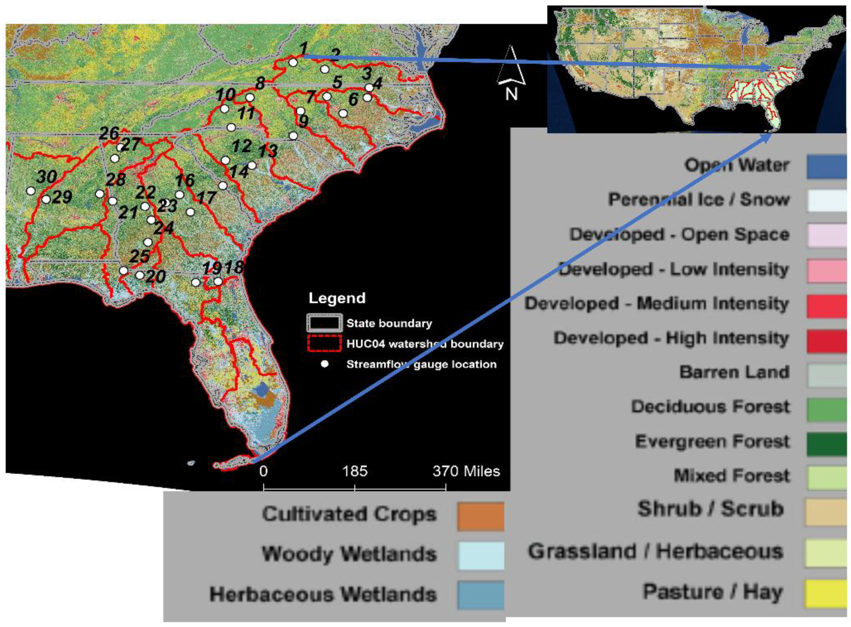
2.1. Study Region

Southeast Atlantic and Gulf Coast (Hydrologic Region 3), the study region, is 1 of the 21 hydrologic regions in the US [14]. The hydrologic region has multiple river basins along the coast with a total area of 721,520 square kilometers of drainage that ultimately discharges into: (a) the Atlantic Ocean within and between the states of Virginia and Florida; (b) the Gulf of Mexico within and between the states of Florida and Louisiana; and (c) the associated waters [15]. The study region has experienced rapid land use/land cover change [16,17,18,19]. The details of the changes are elaborated in the next section (Results and Discussion). The hydrologic region has 18 subregions with 137 hydropower plants that are licensed, exempt, or active and awaiting relicensing [excludes dedicated Pumped Storage Hydropower (PSH) plants and plants with mixed capabilities [20].
The SEUS is physiographically diverse, although dominated by a broad coastal plain [21]. The region includes portions of 16 different Omernik’s ecoregions while providing breeding habitat for 580 terrestrial vertebrate species (e.g., amphibians, birds, mammals, and reptiles), many of which are endemic and/or endangered [22]. The ecoregions include: the blue ridge, piedmont, southeastern plains, middle Atlantic and southeastern coastal plains [23]. The region is a biodiversity hotspot [3] and produces much of the nation’s timber and wood pulp supplies along with cotton, peanuts, citrus, and specialty crops [24].
The SEUS is characterized by a humid, subtropical climate [18]. The region receives ample rainfall throughout the year [25]. Despite this, the region has experienced recurring droughts, which have prompted water use restrictions and induced interstate water conflicts [26]. Much of the region has little seasonality in precipitation, but strong seasonality in runoff owing to high rates of summer evapotranspiration [21]. Additionally, this region is vulnerable to a number of climate-driven events, including sea-level rise, catastrophic floods, heat waves, winter storms, tropical cyclones, and tornadoes [27]. Furthermore, the SEUS often suffers from low surface water availability due to frequent occurrences of La Niña, which brings warm, dry conditions between the months of October and April [26].

2.2. Data Used

Long-term USGS gauging stations in the SEUS were chosen for this study. Initially, 38 USGS gauging stations in Hydrologic Region 3 that had at least 90 years of mean-daily discharge data were identified. The data were downloaded from the USGS National Water Information System (NWIS) Web Interface webpage [28]. After analysis, it was determined that mean-daily discharge data between approximately 1893 (the first year of record for any station) and 1939 have numerous data-gaps at multiple stations. Finally, for this study, mean-daily discharge data from 1 January 1939 to 31 December 2017 (78 years) were selected and used for analysis in Hydrologic Region 3. Table 1 lists the available information about the 30 stations [e.g., USGS Station Number (on map), USGS ID, USGS Station Name, Latitude, Longitude, river mile of station, and drainage area above gauge], while Figure 1 shows their location.
Monthly temperature and precipitation simulations from 19 global climate models for the SEUS region at a 1° × 1° grid scale were used. The data for the states of Alabama, Florida, Georgia, Mississippi, North Carolina, South Carolina, and Tennessee were downloaded (http://gdo-dcp.ucllnl.org/downscaled_cmip_projections/). The period of the temperature data was 1950–2100 for two future scenarios [representative concentration pathways (RCPs) RCP4.5 and RCP8.5] [29]. More details of the data can be obtained from [5,29,30]. Changes in temperature and precipitation observed from literature were used in the meta-analysis. More details of the meta-analysis can be obtained from [5].
The descriptions of streamflow gauge locations are presented in Table 1. The details of land cover data can be obtained from [31].

2.3. Methods

The following steps were carried out in the study.
  • Download data from the 30 USGS gauging stations. The missing data were estimated using a simple average where the number of consecutive missing days was less than 2. Linear regression was used when there were more than 2 consecutive days missing. Details of the missing table can be obtained from the Supplementary Materials (Table S2).
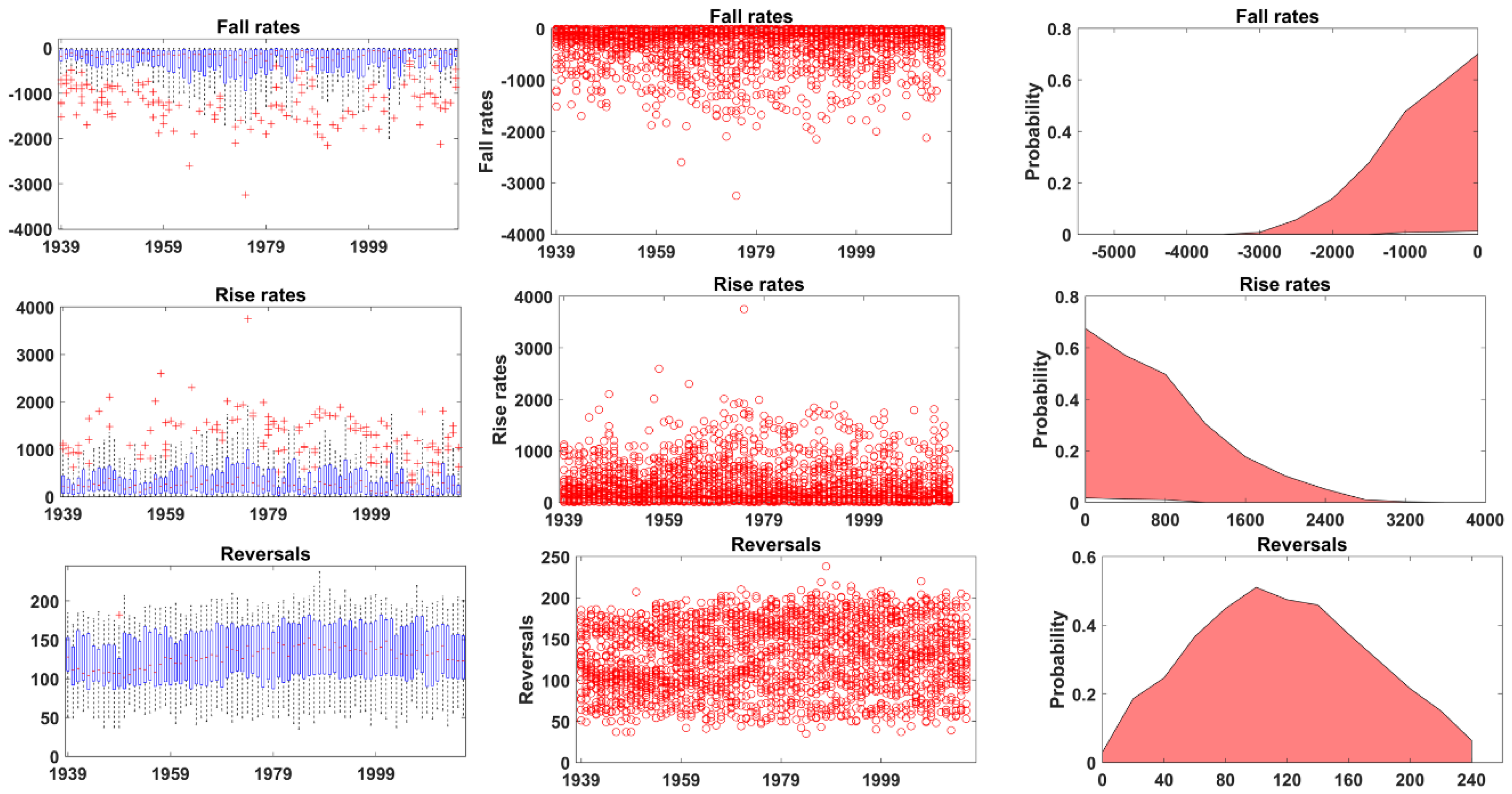
  • Estimate relatively common hydrologic characteristic parameters [2,32] that are strongly correlated to aquatic ecosystem species survival, diversity, richness, habitat maintenance, integrity, and sustainability using the IHA program [2,32]. IHA processes the mean-daily discharge data (input) using a compilation of functions and routines to provide 31 annual and monthly hydrologic characteristics and parameters that describe flow central tendency, variability, magnitudes, timing, frequency, duration, rise and fall rates, and reversals and extremes (outputs). The description of the IHA output variables used in this study and some of its influence on ecosystem functions and processes is presented in Table 2.
  • Analyze the 31 IHA parameters using boxplots and probability density frequency (pdf) plots.
  • Identify the drivers of changes and alterations in streamflow in the study region from published literature.
  • Identify the various change points in streamflow observed from published literature.
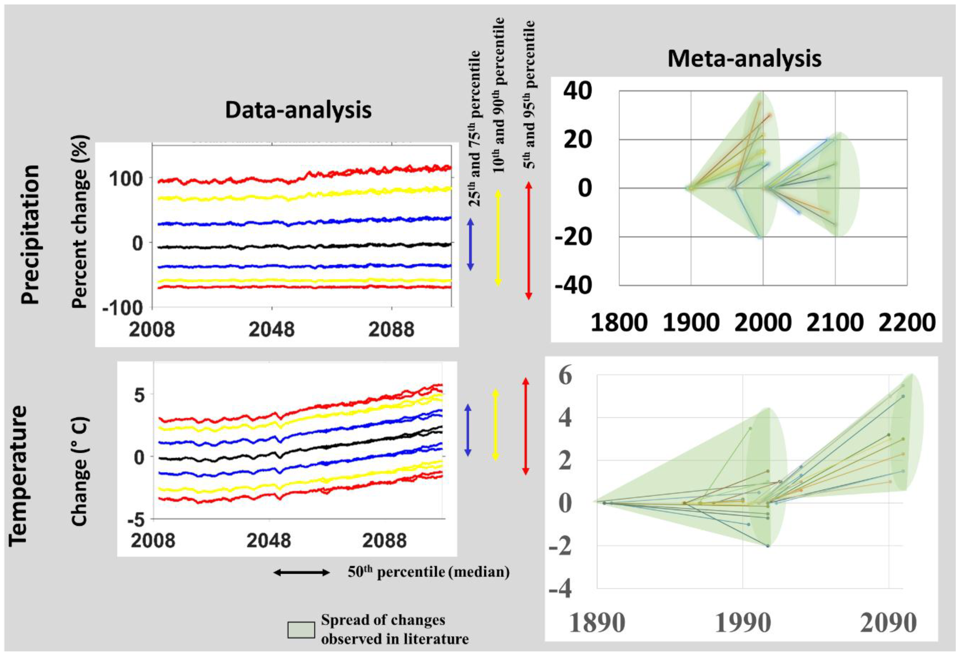
  • Synthesize the climate of the SEUS in terms of temperature and precipitation changes observed from an earlier study using meta-analysis and data analysis of global climate data.
  • Develop a conceptual map of impacts of selected stressors and changes in hydrology and climate for selected periods.

3. Results and Discussion

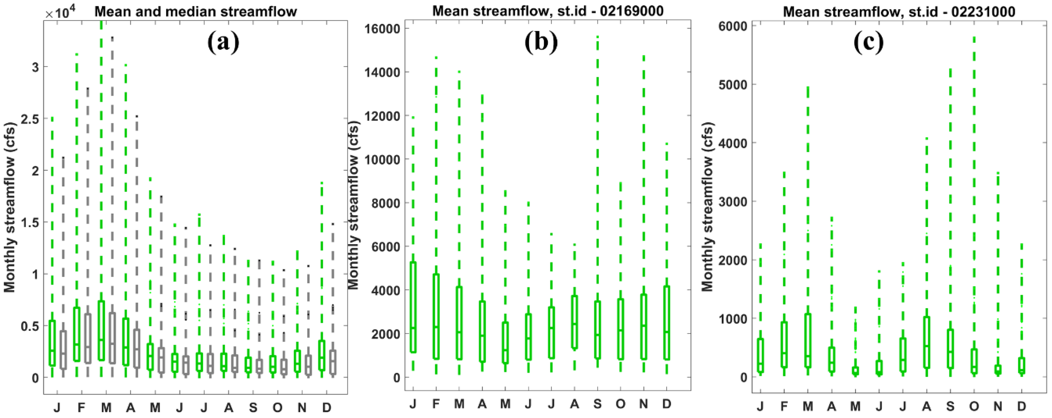
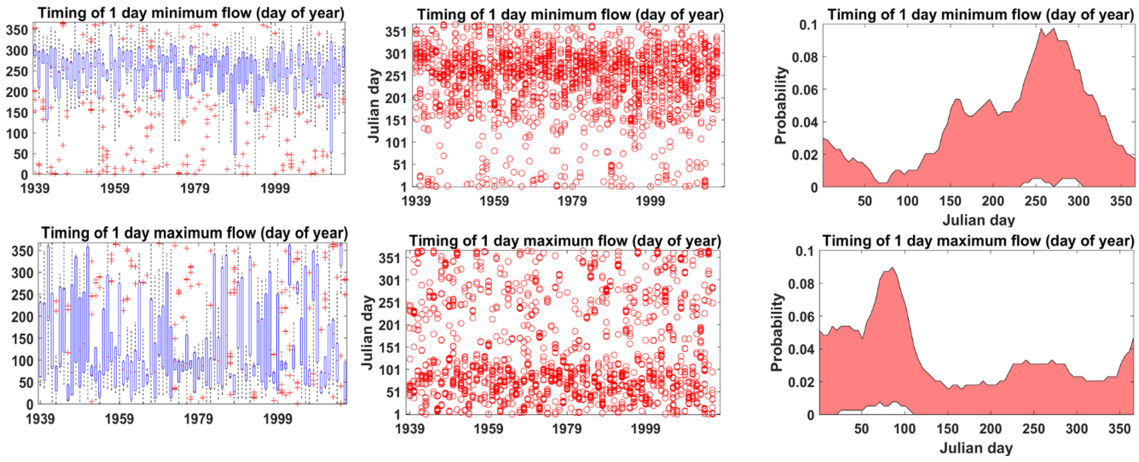
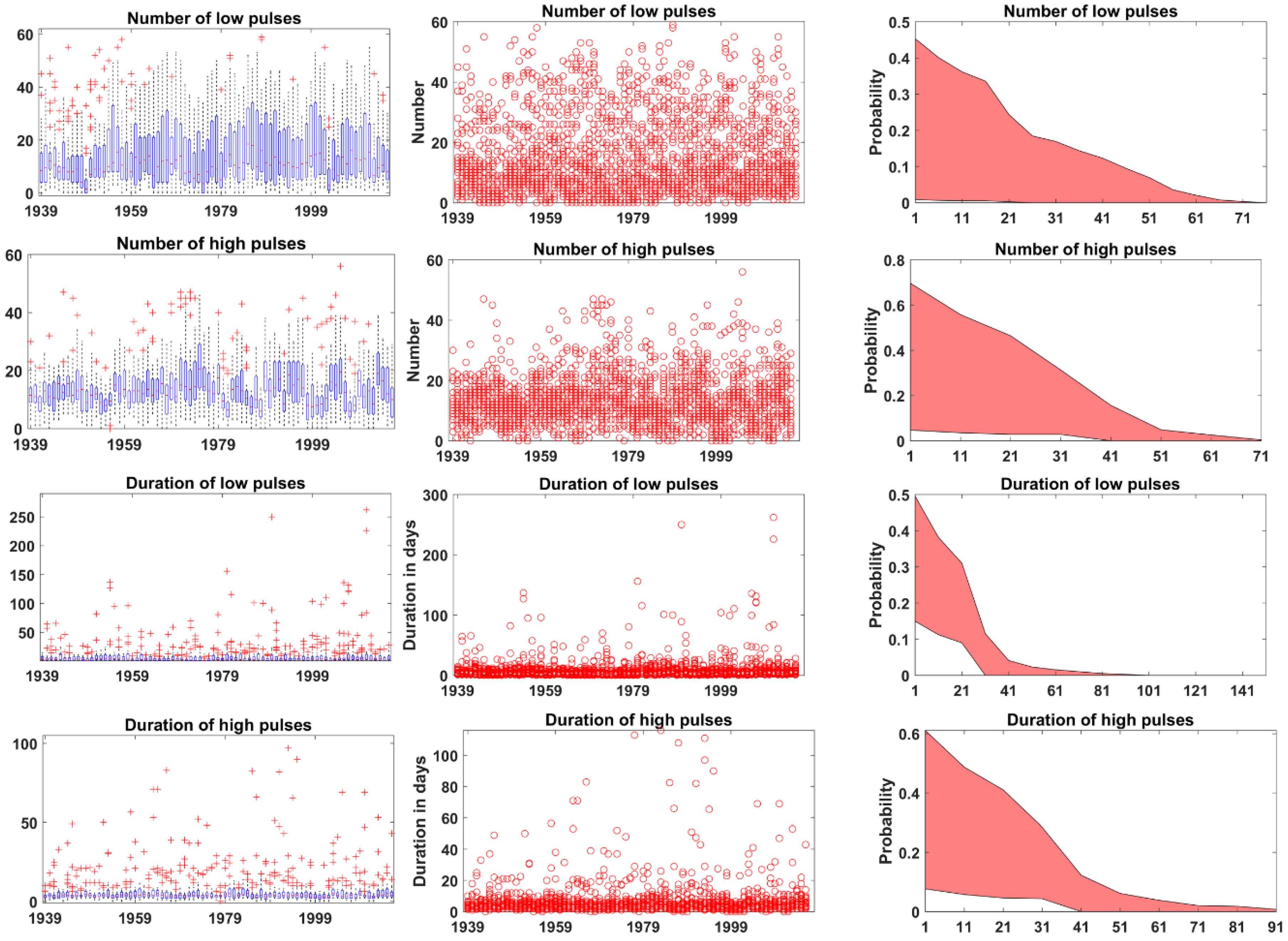
3.1. Overview of the Hydrological Characteristics of Streamflow in the SEUS during 1939–2016

Critical components of the flow regime include the magnitude and seasonal pattern of flows; timing of extreme flows; the frequency, predictability, and duration of floods, droughts, and intermittent flows; daily, seasonal, and annual flow variability; and rates of change in discharge events [34,35]. Boxplots of monthly streamflow data for all 30 stations show seasonality (Figure 2a, green boxes show means and grey boxes show median flows). Generally, among the stations, median flows and variability are highest during the spring season in March (Figure 2a). Flows and distributions in March and April were greater than other months and have the largest range or variability by month of the year. A few exceptions are Saluda River near Columbia, SC, USA (Figure 2b) and St. Mary’s River near Macclenny, FL, USA (Figure 2c). Generally, flow statistics (maximum, 95th percentile, 75th percentile, 25th percentile, 5th percentile, minimum, standard deviation, and interquartile range) follow a similar pattern (Figure S1 in Supplementary Materials). The high flows during the latter part of the year are often associated with hurricane season. High flows in the spring are attributable to the spring low-pressure/storm systems moving through the area, whereas low flows in the fall occur during the post-hurricane and pre-winter-cold-front period (October–December). The lowest long-term median flows are 49 and 101 cubic feet per second (cfs). The drainage areas of the stations ranged from 66.7 mi2 (Linville Rivers, in NC, USGS station 02138500) to 17,200 mi2 (the Apalachicola River at Chattahoochee, FL, USGS station 02358000).
The structure and function of riverine ecosystems, as well as the adaptations of their constituent freshwater and riparian species, are determined by patterns of variation in streamflow [34]. Hydrological characteristics of low flows in all the 30 stations were represented using five indicators for 1-, 3-, 7-, 30- and 90-day minimum streamflow using annual boxplots and PDF plots for the 30 stations (Figure S2 in Supplementary Materials). The plot of the area between the 5th and 95th percentile values for 1- and 90-day minimum streamflow among the 30 stations during 1939–2016 are provided in Row 1 of Figure 3. The five-year moving average of annual one-day minimum streamflow among the 30 stations was 4218 cfs. It increased to 6139 cfs for the 90-day minimum streamflow during 1939–2016. Rolls and Leigh [36] synthesized the literature to outline four mechanistic links between these low flow attributes and the processes and patterns within riverine ecosystems that often are likely to overlap or occur simultaneously. This potentially results in synergistic and complex effects. The four links they observed were that low flows: (1) control the extent of physical aquatic habitat, thereby affecting the composition of biota, trophic structure, and carrying capacity; (2) mediate changes in habitat conditions and water quality, which in turn, drive patterns of distribution and recruitment of biota; (3) affect sources and exchange of material and energy in riverine ecosystems, thereby affecting ecosystem production and biotic composition; and (4) restrict connectivity and diversity of habitat, thereby increasing the importance of refugia and driving multiscale patterns in biotic diversity.
Hydrological characteristics of high flows in all 30 stations were represented using five indicators, namely 1-, 3-, 7-, 30- and 90-day maximum streamflow, using timeseries and PDF plots for the 30 stations (Figure S3 in Supplementary Materials). In Row 2 of Figure 3, the variation between 5th and 95th percentile values for 1- and 90-day maximum streamflow among the stations during the period was observed on average between 84,498 cfs and 19,637 cfs, respectively, during 1939–2016. Truscott and Soulsby [37] stated a few mechanistic links between these high flow events (e.g., short term flood pulses) and the processes and patterns within riverine vegetation, such as that high flow events: (1) shape riverine landscape heterogeneity, productivity and nutrient status, and the composition and structure of riparian vegetation; (2) facilitate the establishment of non-native species and, therefore, riparian habitat can be susceptible to plant invasions; and (3) alter the competitive balance between native and non-native species redistributing nutrients, which facilitate the colonization of non-native species. Intermittent rivers function differently from their perennial counterparts [38] due to these mechanistic links between flow attributes and the processes and patterns within riverine ecosystems. For example, they differ with respect to biogeochemical fluxes and may have substantial impacts on carbon and nutrient fluxes [38]. The magnitudes of the high and low flows were correlated to the drainage area (Row 3 in Figure 3).
The timing of the occurrence of particular water conditions can determine whether certain life cycle requirements are met or influence the degree of tress or mortality associated with extreme water conditions such as floods or droughts [2]. The analysis of the timing of one-day minimum and maximum flow among the stations revealed the distribution of the Julian day at which they occurred and the year to year variability (boxplots and scatter plots, Columns 1 and 2 in Figure 4). From the PDF distribution, it can be observed that Julian Days ~270–280 (last week of September and first week of October) and ~70–80 (second and third weeks of March) had the highest distribution of one-day minimum and maximum flows among the stations as well as highest variation among the 30 stations in the region (Column 3 in Figure 4). No significant relationship was observed between the timing and the drainage area (Figure S4 in Supplementary Materials). The timing of extreme annual low flows will be useful in the predicting and avoiding of stress for organisms due to low flows, while the timing of high flows provides spawning cues for migratory fish [33].
The frequency and duration of the occurrence of specific water conditions together portray the pulsing behavior of environmental variation within a year, and provide measures of the shape of these environmental pulses [2]. The number and duration of the high/low pulses had a similar interquartile range of 5–20 and 0–5 days, respectively (Columns 1 and 2 in Figure 5). However, the inter-annual variability and the range between the maximum and minimum values were higher for the number and duration of low pulses (0–60 and 0–250) in comparison to the high pulses (0–50 and 0–100), respectively. The pulsing behavior followed an exponential distribution (Column 3 in Figure 5). In general, smaller values for the number of pulses and duration had a higher probability of occurrence among the stations with high pulses. This can be observed by the greater spread between the 5th and 95th percentile values for the lower number of pulses and duration when compared to the higher ones. The variability in the number of high flows during extreme drought years is smaller (e.g., dust bowl period and back to back droughts during the 1950s). Water conditions such as droughts or floods may be tied to reproduction or mortality events for various species, thereby influencing population dynamics [2]. This knowledge will be helpful to understand the frequency and magnitude of soil moisture stress and availability of habitat for flora and fauna in the floodplain, and to understand the hydraulic effects such as bedload transport, channel sediment distribution, and the duration of its disturbance [33].
The rate of rise, fall and reversals in the water conditions may be tied to the stranding of certain organisms along the water’s edge or in ponded depressions, or they may be tied to the ability of plant roots to maintain contact with phreatic water supplies [2]. Among the stations, the rise and fall rates varied between 1 and 4000 and −4000 and 1, respectively (Rows 1 and 2 in Figure 6), while the reversal varied between 1 and 250 (Row 3 in Figure 6). The boxplots and scatter plots provide a measure of the rate of inter-annual change, while the rates themselves provide the intra-annual environmental change. The probability of the occurrence of the rise, fall and reversal rates are highest in the ranges 1–50, 1–40 and 80–120, respectively (Column 3 in Figure 6). Knowledge of these changes from one day to the next can be useful to understand the drought stress on plants as well as desiccation stress on the low-mobility of stream edge organisms [33].
The knowledge of the various IHA flow parameters would be useful in understanding the synergistic and complex effects of these mechanistic links while maintaining the water quality, ecosystem processes, and functions sustainably. For example, while meeting the spawning flow targets in the rivers, we can prevent dissolved oxygen impacts of hypoxic swamp water drainage on waters in the main stem of the river. The parameters would support planning and management of flow targets by aiding in the step-down process during high flows and step-up process during low flows. A specific example is in the Roanoke River during the spawning season for anadromous fishes during 1 April–15 June [9]. Knowledge of the IHA high flow parameters would be useful in the step-down process by holding water in the floodplain to meet spawning flow targets. The frequency, magnitude, duration, timing, and spatial extent of flow events are universal drivers of ecological integrity in riverine ecosystems and apply to events of both high and low flow magnitude [36].

3.2. Overview of the Climate Change and Variability in the SEUS during 1950–2100

Climate change can be represented using changes in variables such as temperature and precipitation. These changes cause alterations in the streamflow of a region [7]. An earlier study observed the changes in temperature and precipitation in the SEUS through syntheses of literature (meta-analysis) and simulations from outputs from ~19 (data analysis) Coupled Model Intercomparison Project (CMIP5) Global Climate Models (GCMs) [39]. In general, the meta-analysis of literature in the SEUS revealed that the precipitation changes observed range from −30% to +35% and temperature changes from −2 °C to 6 °C by 2099 (Figure 7, Column 2). The fiftieth percentile of the GCMs predict no precipitation change and an increase in temperature of 2.5 °C in the region by 2099 (Figure 7, Column 1). Among the GCMs, the 5th and 95th percentile of precipitation changes range between −40% and 110% and temperature changes between −2 °C and 6 °C by 2099 (Figure 7, Column 1). The causes for precipitation change are very complex [19]. The data analysis in the SEUS included the seven states of Alabama, Florida, Georgia, Mississippi, North Carolina, South Carolina, and Tennessee. In the meta-analysis of changes, the literature included had multiple boundaries define the SEUS. Some studies include the same seven states, while some had additions or exclusions of one or more states. There are three contributors to precipitation formation, i.e., atmospheric circulation dynamical systems, water vapor transport, and vertical thermal stability [19]. The warm/cold El Niño Southern Oscillation (ENSO) events are characterized by colder and wetter/warmer and drier boreal winter and spring seasons in the SEUS, with the magnitudes of these anomalies, however, decrease as one moves northward within the SEUS [39]. For example, they observed that ENSO influences the winter hydrology of the SEUS with the variability of streamflow in the southern watersheds (over Florida) showing a stronger relationship than the northern watersheds in the region. During La Niña events, reduced precipitation and streamflow are observed for a large portion of the stations in the SEUS, especially for the December-January-February (DJF) and March-April-May (MAM) seasons [40]. The climate change and variability not only impact the river flow but also its water quality which are both major determinants of river ecosystem conditions and the resulting benefits (e.g., factors such as light, temperature, channel morphology, and species interactions).

3.3. Drivers of Changes and Alterations in Streamflow in the SEUS

Streamflow is one the most important variables controlling and maintaining aquatic ecosystem integrity, diversity, and sustainability. Human control of streamflow is now ubiquitous and growing rapidly. Alteration of a streamflow regime, through the construction and operation of dams and weirs, is arguably the most significant threat to the ecological health of the world’s rivers [41]. Subtle alteration of streamflow regimes, that can be caused by water diversion or direct extraction from free-flowing river systems for agricultural and urban water use (i.e., drainages without substantial instream dams), may influence the characteristics of hydrologic impacts and ecological responses [42]. The following drivers impact the streamflow regime as well as stress the river systems in the SEUS: climate change, land use/land cover change (e.g., conversion of forests to farmland, regeneration of forests from farmland, forest/farmland fragmentation, and urbanization), sedimentation, population increase, economic development, and manmade structures built on streams. These drivers also alter the climatic conditions of the SEUS.
As some of the drivers of change, hydromorphological pressures and alterations in streamflow in the SEUS are discussed briefly. The SEUS has experienced rapid land use/land cover change with multiple primary drivers: timber harvesting and conversion of forests to agriculture during the 19th and early 20th centuries which reached a low in ~1920 [19]; regeneration of forests from farmland following the Great Depression of the 1930s [7]; forest fragmentation caused by the economic boom during the 1980s to 2000s; [17] and, recently, the conversion of agricultural land use to urban/suburban development [18]. These land use/land cover changes can affect the regional hydrologic and climatic conditions through changing the surface energy, water fluxes, soil hydraulic property, and surface roughness [19]. Human population has dramatically increased since 1940, which has changed land and water use over time. The rise in urban population is accompanied by an increase in urbanized areas. For example, population increases of between 25% and 35% from 1970–2000 were found in the Lower Ocmulgee, Lower Oconee, Ohoopee, and Altamaha watersheds [10]. Increasing trends of exurban development and suburban residential development in previously rural landscapes (rural suburbanization) fragment the region’s agriculture and forested lands. This land transformation alters the hydrologic response of the land via changes in vegetation, impervious landcover, and drainage; increases withdrawals from surface and groundwater to support increased demands; and alters the hydrologic cycle via water and wastewater infrastructure that can alter both recharge and subsurface drainage [43]. Additional impacts of urbanization processes are the growing areas of impervious (sealed) surfaces (e.g., parking lots, asphalt, roofing, and concrete and gravel roads) which prevent rainwater infiltration into the soil and cause its direct runoff to storm drain systems.
Hydromorphological pressures comprise all physical alterations due to the modifications of their shores (e.g., riparian and littoral zones, water level and flow, navigation, flood prevention building reservoirs) as well as to meet the demand for multiple uses (agriculture, urbanization, hydropower, mineral extraction, fishing, tourism, etc.) [44]. Although river flow derives ultimately from precipitation, at any given time and place, a river’s dominant flow pressure are derived from some combinations that help to determine both the supply of water and the pathways by which precipitation reaches the channel. Example of combination parameters include: surface water, soil water, groundwater, climate, geology, topography, soils, vegetation, land use/land cover, etc. [1]. Many different methods have been applied to reveal dominant processes/pressures in river basins such as chaos theory, wavelet theory, circular statistics, and time series analysis techniques [45]. Identifying the reasons for significant changes would often require a “reference” with a natural flow regime. Determining the reasons is challenging, because there is currently insufficient knowledge in defining “significant change” and they carry considerable uncertainty [46]. The dominant pressures could vary with high/average/low flows. During the latter half of the 19th to mid-late 20th century, the US Army Corps of Engineers constructed hydrologic structures on many of the free-flowing rivers in the SEUS for flood relief, power generation purposes, and, in some cases, water supply (Atlanta). Alteration of a streamflow regime through the construction and operation of dams and weirs may produce hydrologic impacts (e.g. “hydropeaking”), which typically change sub-daily flow variability due to changes in energy demand and power station operation. For example, the Tallapoosa’s flow regime in certain reach typically fluctuates between extreme low and high flows corresponding to patterns in power generation [12]. Land conversion (e.g., urbanization) and stream channelization can also increase peak discharge, with shorter flood durations, and decrease baseflows, resulting in flashier flows. Heavy water extraction from free-flowing streamflow due to agricultural and urban water use may also produce hydrologic impacts that are similar to “hydropeaking” and is often a neglected driver of alterations in streamflow [42]. The methods/parameters of hydromorphological pressures (e.g., hydropeaking) will need to have significant differences between pre- and post-pressure to have large confidence bands to account for this uncertainty [46]. In general, the drivers often include a combination of changes in streamflow, and it is often difficult to separate the effects of individual drivers [47].

3.4. Change Points in Streamflow and Climate in the SEUS

Many rivers in the US have had a significant reduction in flood flows due to dams. The degree of flood flow alteration increases as the size of the river increases, with a 29% reduction of mean annual flows in large rivers, 15% in medium rivers, and 7% in small rivers [48]. Measures of flow alteration and criteria for establishing reference conditions were variable [1]. Additionally, identifying the exact points of changes can be challenging due to the existence of multiple drivers of change, hydromorphological pressures, and alterations in streamflow in the region. These changes have been observed using single station data or using clusters of change points from multiple station data. Each of these have their own advantages and disadvantages. When only a single stream gauge is analyzed, it is difficult to distinguish whether a change point is due to changes in drivers (e.g., climate) or more direct changes such as modifications to the instruments used to measure streamflow [49]. Studies have documented that streamflow exhibits a step change around 1970, and that the observed streamflow change is in concert with a change in precipitation in the region [50,51,52]. Spatial clusters of change points have been observed in the SEUS’s mean normalized streamflow and precipitation during 1957–1998 [53]. The changes in the 1950s could be attributed to back-to-back droughts in the region [54]. Spatial distribution of stations with step changes occurring at different time intervals vary with seasons [19]. Spatial clusters of seasonal breaks reveal that the spring season is significantly earlier (late 1980s–early 1990s) than all other seasons (break in 1998–1999) [52]. The year of streamflow regulation has been observed as alternation points which varies with the station. Additionally, the streams are regulated due to hydropower generation in the region. Recent statistics show that in the 12 subregions (HUC-04) there are 142 hydropower, PSH, and mixed facilities that are licensed, exempt, or currently active but awaiting relicensing [20]. Identifying the year of regulation in each of them can be challenging. Attributing the hydrological changes in the SEUS associated to climate change, changes associated to other aspects of human activity, and the changes discussed in this section (based on earlier results, e.g., 1957, 1970, and 1998) for the SEUS can be a continuation of this study and is deferred for future work.
The alteration disrupts the longitudinal continuity of fluvial ecosystems, often compromising the biotic integrity of rivers by restricting the downstream transport of sediments, trophic resources, the migration of lotic fauna (e.g., fish), modifying downstream channel morphologies, the physicochemical properties (e.g., dissolved oxygen and stream temperature variability). The flow alterations are associated with ecological change, and the risk of ecological change increases with increase in the magnitude of flow alteration [1]. Gillespie et al. [55] observed evidence of relationships among flow, biota, water quality, and ecosystem responses under flow modifications. They identified that research was primarily focused on traditionally monitored ecological groups (e.g., fish) and the importance of site-specific factors (e.g., climate).

3.5. Conceptual Map of Selected Drivers of Changes and Alterations in Streamflow and Climate in the SEUS

Figure 8 shows a conceptual map of the impacts of selected drivers and changes in hydrology and climate in the study region for the late 19th century to the present day using DPSIR framework for three types of land use/land cover changes for three periods. In the framework, the drivers are land use/land cover change, climate change, and variability. They apply pressure on the region (e.g., forest restoration, Row 1 in Figure 8, grey arrows). The state of the system is represented using variables (e.g., runoff) and the change in the state of the systems are identified (Row 2 in Figure 8 in green color) using measured variables (e.g., streamflow) and its characteristics (e.g., IHA parameters). The changes then impact climate (Row 4 in Figure 8), and the system responds to the changes in the state (Row 4 in Figure 8). The 31 IHA parameters estimated could provide useful information on different components of the DPSIR ecosystems for the region (e.g., impact, response, and state).
The variability of atmospheric temperature is a major driver of water temperature, which is important for the distribution of aquatic species and the biogeochemistry of fluvial ecosystems, while the precipitation regime governs the hydrologic regime of fluvial ecosystems and the catchment run-off processes [50]. In general, forested catchments had higher evapotranspiration than grass pastures, with few exceptions. Replacing trees with grass cover generally increases runoff by decreasing evapotranspiration [47]. Forest restoration increased surface roughness and reduced the southerly winds. This caused a decrease in July precipitation (due to weaker moist transport), while causing reduced northerly winds resulting in an increase in January precipitation (due to weaker dry and cold airflows) [16]. Reduced regional farm and forest productivity may result from altered rainfall patterns and increased climate variability [24]. From a forest-based water production perspective, a 2 °C increase in temperatures can decrease water yield by 11%, and a 10% reduction of precipitation can lead to a 20% decline in water yield in loblolly pine forests [56]. In general, for most of the SEUS a 1% increase in precipitation leads to a 1.5–2.5% increase in runoff, while some areas in the southeast get up to a 4% increase in streamflow, implying less evaporation and/or storage capacity [52]. The reduction of water yield combined with increased population and land use changes may increase water stress by 10% by 2050 [56].
In the region, a significant relationship was found between the frequency of heavy precipitation and high streamflow events both annually and during the months of maximum streamflow [57]. It was observed that two factors contributed to finding such a relationship: (1) the relatively small contribution of snowmelt to heavy runoff in the SEUS (compared to the west); and (2) the presence of a sufficiently dense network of streamflow (except in Florida) and precipitation gauges available for analysis. The use of ENSO in water resources management is often limited to the boreal winter season for the SEUS, as its signal is well reflected in hydrological responses [40]. Spatial distribution of the unimpaired stations (periods ranged from 30–109 years) with shifts across the SEUS using Pettitt’s test over the duration of a water-year (i.e., fall-summer). Significant decreasing trends are observed in the SEUS [19]. When land cover changes and surface albedo changes (i.e., solar radiation absorbed on the ground), this will, in turn, change the latent heat energy and hydrological processes of the region [19]. For example, urban-induced rainfall can be a result of the urban heat island effect (a warming of the local climate due to changes in land cover, drainage, shading, and albedo), and these heat islands can alter convection of air masses in urban areas. In addition, urban surface roughness and the urban canopy (buildings, infrastructure, or trees) can affect air circulation, while the presence of enhanced aerosols in urban areas may also influence the local climate [18]. Explaining the reason(s) for the significant differences in the changes and alterations in streamflow and climate, as well as defining the ecological impacts of multiple stressors, is challenging. These multiple drivers and stressors may have simultaneous effects and attributing causality is problematic [42].

4. Conclusions

Streamflow has been called the “master variable” that orchestrates pattern and process in rivers. The southeastern United States (SEUS) is a biodiversity hotspot, and the region has been underrepresented in hydroclimatic research. Studies in the SEUS have been mostly localized on specific rivers, reservoir catchments and/or species, but the overall region has not been assessed for multiple hydrologic characteristic parameters for the long-term period of 1939–2016. The objectives of the study were to (1) provide an overview of the multiple hydrologic characteristic parameters of streamflow in the region for a longer period and in multiple river basins; and (2) develop a conceptual map of the impacts of selected stressors and changes in hydrology and climate in the SEUS.
A seven step procedure was used to accomplish these objectively: Step 1: Download data from the 30 USGS gauging stations. Step 2: Estimate relatively common hydrologic characteristics and parameters that are correlated to the ecosystem. Step 3: Analyze the 31 IHA parameters using boxplots, scatter plots, and PDFs. Step 4: Identify the drivers of changes and alterations in streamflow from published literature. Step 5: Identify the various change points in the streamflow observation literature. Step 6: Synthesize the climate of the SEUS in terms of temperature and precipitation changes. Step 7: Develop a conceptual map of the impacts of selected stressors and changes in hydrology and climate for selected periods using the Driver–Pressure–State-Impact–Response (DPSIR) framework.
In general, the meta-analysis of literature in the SEUS revealed the precipitation changes observed ranged from −30% to +35% and temperature changes from −2 °C to 6 °C by 2099. The fiftieth percentile of the simulations from Global Climate Models (GCMs) predict no precipitation change and an increase of 2.5 °C temperature in the region by 2099. Among the GCMs, the 5th and 95th percentile of precipitation changes range between −40% and 110% and temperature changes between −2 °C and 6 °C by 2099. In addition to climate, the region has experienced a number of rapid land use/land cover changes with multiple primary drivers of change, such as: (1) the conversion of forests to agriculture during the 19th century and early 20th century, which reached a low in ~1920; (2) the regeneration of forests from farmland following the Great Depression of the 1930s; (3) forest fragmentation caused by the economic boom in the 1980s–2000s; and (4) recently, the conversion of agricultural land use to urban/suburban development. The years 1957, 1970, and 1998 were some of the change points documented in literature for precipitation and streamflow in the region.
A conceptual map was developed of the impacts of selected drivers and changes in hydrology and climate in the study region for three land use/land cover categories in three different periods (late 19th century to the present day) using DPSIR framework. The 31 IHA parameters estimated could provide useful information on different components of the DPSIR ecosystems for the region (e.g., impact, response, and state). Attributing the hydrological changes associated to climate change, changes associated to other aspects of human activity, and the changes due to change points (e.g., 1957, 1970, and 1998) for the SEUS, and synthesizing them for each river basin, can be a continuation of this study and is deferred for future work. Additionally, identifying the effects of individual drivers and quantifying them are also deferred for future work.

Supplementary Materials

The following are available online at https://www.mdpi.com/2306-5338/5/3/42/s1. Figure S1: Monthly distribution of streamflow statistics from the 30 stations during the study period 1939–2016, Figure S2: Boxplot of annual distribution of magnitude of low flow streamflow statistics from the 30 stations during the study period 1939–2016, Figure S3: Boxplot of annual distribution of magnitude of low flow streamflow statistics from the 30 stations during the study period 1939–2016, Table S1: Documentation of the literature was reviewed using search words (in quotes) and the corresponding number of studies (in parenthesis), Table S2: Summary of missing data by station and missing-time period intervals.

Author Contributions

A.A.: Validation, Formal Analysis, Investigation, Resources, Data Curation; Writing—Original Draft Preparation: A.A., C.C. and C.B.

Acknowledgments

This material is based upon work partially supported by the National Science Foundation under Grant No. 1735235 awarded as part of the National Science Foundation Research Traineeship (NRT), USDA-NIFA capacity building grant 2017-38821-26405, USDA-NIFA Evans-Allen Project, Grant 11979180/2016-01711, USDA-NIFA Grant No. 2018-68002-27920 and Department of Energy Minority Serving Institution Partnership Program (MSIPP) managed by the Savannah River National Laboratory under SRNS contract DE-AC09-08SR22470. Christy Crandall was an NRT trainee during August, 2017 to January 2018 while carrying the work. The authors express their gratitude to the five anonymous reviewers for their constructive comments and suggestions on the earlier draft of the paper. Finally, the authors would like to acknowledge Alison Schardl for editing support. The support from Anjali Sharma in obtaining literature is acknowledged.

Conflicts of Interest

The authors declare no conflict of interest.

References

  1. Poff, N.L.; Richter, B.D.; Arthington, A.H.; Bunn, S.E.; Naiman, R.J.; Kendy, E.; Acreman, M.; Apse, C.; Bledsoe, B.P.; Freeman, M.C.; et al. The ecological limits of hydrologic alteration (ELOHA): A new framework for developing regional environmental flow standards. Freshwater Biol. 2010, 55, 147–170. [Google Scholar] [CrossRef]
  2. Richter, B.D.; Baumgartner, J.V.; Powell, J.; Braun, D.P. A method for assessing hydrologic alteration within ecosystems. Conserv. Biol. 1996, 10, 1163–1174. [Google Scholar] [CrossRef]
  3. Cartwright, J.M.; Wolfe, W.J. Insular Ecosystems of the Southeastern United States—A Regional Synthesis to Support Biodiversity Conservation in a Changing Climate; Professional Paper; US Geological Survey: Reston, VA, USA, 2016.
  4. Lynch, A.J.; Myers, B.J.; Chu, C.; Eby, L.A.; Falke, J.A.; Kovach, R.P.; Krabbenhoft, T.J.; Kwak, T.J.; Lyons, J.; Paukert, C.P.; et al. Climate change effects on North American inland fish populations and assemblages. Fisheries 2016, 41, 346–361. [Google Scholar] [CrossRef]
  5. Anandhi, A.; Bentley, C. Predicted 21st Century Climate variability in Southeastern U.S. using downscaled CMIP5 and meta-analysis. Catena 2018, in press. [Google Scholar] [CrossRef]
  6. Martin, T.A.; Adams, D.C.; Cohen, M.J.; Crandall, R.M.; Gonzalez-Benecke, C.A.; Smith, J.A.; Vogel, J.G. Managing Florida’s Plantation Forests in a Changing Climate. In Florida’s Climate: Changes, Variations & Impacts; Florida Climate Institute: Gainesville, FL, USA, 2017. [Google Scholar]
  7. Engström, J.; Waylen, P. The changing hydroclimatology of Southeastern US. J. Hydrol. 2017, 548, 16–23. [Google Scholar] [CrossRef]
  8. White, J.C.; Hannah, D.M.; House, A.; Beatson, S.J.; Martin, A.; Wood, P.J. Macroinvertebrate responses to flow and stream temperature variability across regulated and non-regulated rivers. Ecohydrology 2017, 10. [Google Scholar] [CrossRef]
  9. Pearsall, S.H.; McCrodden, B.J.; Townsend, P.A. Adaptive management of flows in the lower Roanoke River, North Carolina, USA. Environ. Manag. 2005, 35, 353–367. [Google Scholar] [CrossRef] [PubMed]
  10. Weston, N.B.; Hollibaugh, J.T.; Joye, S.B. Population growth away from the coastal zone: Thirty years of land use change and nutrient export in the Altamaha River, GA. Sci. Total Environ. 2009, 407, 3347–3356. [Google Scholar] [CrossRef] [PubMed]
  11. Engström, J.; Waylen, P. Drivers of long-term precipitation and runoff variability in the southeastern USA. Theor. Appl. Climatol. 2018, 131, 1133–1146. [Google Scholar] [CrossRef]
  12. Fehér, J.; Gáspár, J.; Szurdiné-Veres, K.; Kiss, A.; Kristensen, P.; Peterlin, M.; Globevnik, L.; Kirn, T.; Semerádová, S.; Künitzer, A.; et al. Hydromorphological Alterations and Pressures in European Rivers, Lakes, Transitional and Coastal Waters; Thematic Assessment for EEA Water 2012 Report; European Topic Centre on Inland, Coastal and Marine Waters: Magdeburg, Germany, 2012. [Google Scholar]
  13. Anandhi, A.; Sharma, A.; Sylvester, S. Can meta-analysis be used as a decision making tool for developing scenarios 1 and causal chains in eco-hydrological systems?—Case study in Florida. Ecohydrology 2018, in press. [Google Scholar] [CrossRef]
  14. Seaber, P.R.; Kapinos, F.P.; Knapp, G.L. Hydrologic Unit Maps; USGPO: Washington, DC, USA, 1987.
  15. Bobsein, J. Streamflow Extremes and Climate Variability in Southeastern United. Master’s Thesis, Florida Atlantic University, Boca Raton, FL, USA, May 2015; pp. 425831–425833. Available online: http://fau.digital.flvc.org/islandora/object/fau%3A31265/datastream/OBJ/view/Streamflow_extremes_and_climate_variability_in_Southeastern_United_States.pdf (accessed on 5 May 2015).
  16. Liu, Y. A numerical study on hydrological impacts of forest restoration in the southern United States. Ecohydrology 2011, 4, 299–314. [Google Scholar] [CrossRef]
  17. Griffith, J.A.; Stehman, S.V.; Loveland, T.R. Landscape trends in mid-Atlantic and southeastern United States ecoregions. Environ. Manag. 2003, 32, 572–588. [Google Scholar] [CrossRef] [PubMed]
  18. O’Driscoll, M.; Clinton, S.; Jefferson, A.; Manda, A.; McMillan, S. Urbanization effects on watershed hydrology and in-stream processes in the southern United States. Water 2010, 2, 605–648. [Google Scholar] [CrossRef]
  19. Tamaddun, K.; Kalra, A.; Ahmad, S. Identification of streamflow changes across the continental United States using variable record lengths. Hydrology 2016, 3, 24. [Google Scholar] [CrossRef]
  20. Samu, N.M.; Kao, S.-C.; O’Connor, P.W. 2015 NHAAP Energy Dataset Version 1.0 (v1). Oak Ridge National Laboratory. Available online: http://nhaap.ornl.gov (accessed on 14 May 2018).
  21. Mulholland, P.J.; Best, G.R.; Coutant, C.C.; Hornberger, G.M.; Meyer, J.L.; Robinson, P.J.; Stenberg, J.R.; Turner, R.E.; Vera-Herrera, F.R.; Wetzel, R.G. Effects of climate change on freshwater ecosystems of the south-eastern United States and the Gulf Coast of Mexico. Hydrol. Process. 1997, 11, 949–970. [Google Scholar] [CrossRef]
  22. Martinuzzi, S.; Withey, J.C.; Pidgeon, A.M.; Plantinga, A.J.; McKerrow, A.J.; Williams, S.G.; Helmers, D.P.; Radeloff, V.C. Future land-use scenarios and the loss of wildlife habitats in the southeastern United States. Ecol. Appl. 2015, 25, 160–171. [Google Scholar] [CrossRef] [PubMed]
  23. Napton, D.E.; Auch, R.F.; Headley, R.; Taylor, J.L. Land changes and their driving forces in the Southeastern United States. Reg. Environ. Chang. 2010, 10, 37–53. [Google Scholar] [CrossRef]
  24. Elias, E.; Schrader, T.S.; Abatzoglou, J.T.; James, D.; Crimmins, M.; Weiss, J.; Rango, A. County-level climate change information to support decision-making on working lands. Clim. Chang. 2018, 148, 355–369. [Google Scholar] [CrossRef]
  25. Rose, S. Rainfall—Runoff trends in the south-eastern USA: 1938–2005. Hydrol. Process. 2009, 23, 1105–1118. [Google Scholar] [CrossRef]
  26. Mitra, S.; Srivastava, P. Spatiotemporal variability of meteorological droughts in southeastern USA. Nat. Hazards 2017, 86, 1007–1038. [Google Scholar] [CrossRef]
  27. Ingram, K.T.; Dow, K.; Carter, L.; Anderson, J. Climate of the Southeast United States: Variability, Change, Impacts, and Vulnerability; Inland Press: Detroit, MI, USA, 2013. [Google Scholar]
  28. USGS. The United States Geological Survey (USGS), Water Data for the Nation. Available online: https://waterdata.usgs.gov/nwis (accessed on 16 June 2018).
  29. Van Vuuren, D.P.; Edmonds, J.; Kainuma, M.; Riahi, K.; Thomson, A.; Hibbard, K.; Hurtt, G.C.; Kram, T.; Krey, V.; Lamarque, J.F.; et al. The representative concentration pathways: An overview. Clim. Chang. 2011, 109, 5–31. [Google Scholar] [CrossRef]
  30. Maurer, E.P.; Brekke, L.; Pruitt, T.; Thrasher, B.; Long, J.; Duffy, P.; Dettinger, M.; Cayan, D.; Arnold, J. An enhanced archive facilitating climate impacts and adaptation analysis. Bull. Am. Meteorol. Soc. 2014, 95, 1011–1019. [Google Scholar] [CrossRef]
  31. Homer, C.; Dewitz, J.; Yang, L.; Jin, S.; Danielson, P.; Xian, G.; Coulston, J.; Herold, N.; Wickham, J.; Megown, K. Completion of the 2011 National Land Cover Database for the conterminous United States—Representing a decade of land cover change information. Photogramm. Eng. Remote Sens. 2015, 81, 345–354. [Google Scholar]
  32. Richter, B.D.; Mathews, R.; Harrison, D.L.; Wigington, R. Ecologically sustainable water management: Managing river flows for ecological integrity. Ecol. Appl. 2003, 13, 206–224. [Google Scholar] [CrossRef]
  33. Swanson, S. Indicators of Hydrologic Alteration. Resource Notes No 58. National Science and Technology Center, Bureau of Land Management, 2012. Available online: http://www.blm.gov/nstc/resourcenotes/respdf/RN58.pdf (accessed on 8 June 2018).
  34. Kennard, M.J.; Pusey, B.J.; Olden, J.D.; MacKay, S.J.; Stein, J.L.; Marsh, N. Classification of natural flow regimes in Australia to support environmental flow management. Freshwater Biol. 2010, 55, 171–193. [Google Scholar] [CrossRef]
  35. Kennard, M.J.; Mackay, S.J.; Pusey, B.J.; Olden, J.D.; Marsh, N. Quantifying uncertainty in estimation of hydrologic metrics for ecohydrological studies. River Res. Appl. 2010, 26, 137–156. [Google Scholar] [CrossRef]
  36. Rolls, R.J.; Leigh, C.; Sheldon, F. Mechanistic effects of low-flow hydrology on riverine ecosystems: Ecological principles and consequences of alteration. Freshwater Sci. 2012, 31, 1163–1186. [Google Scholar] [CrossRef]
  37. Truscott, A.M.; Soulsby, C.; Palmer, S.; Newell, L.; Hulme, P. The dispersal characteristics of the invasive plant Mimulus guttatus and the ecological significance of increased occurrence of high-flow events. J. Ecol. 2006, 94, 1080–1091. [Google Scholar] [CrossRef]
  38. Costigan, K.H.; Jaeger, K.L.; Goss, C.W.; Fritz, K.M.; Goebel, P.C. Understanding controls on flow permanence in intermittent rivers to aid ecological research: Integrating meteorology, geology and land cover. Ecohydrology 2016, 9, 1141–1153. [Google Scholar] [CrossRef]
  39. Nag, B.; Misra, V.; Bastola, S. Validating ENSO teleconnections on Southeastern US winter hydrology. Earth Interact. 2014, 18, 1–23. [Google Scholar] [CrossRef]
  40. Wang, H.; Asefa, T. Impact of different types of ENSO conditions on seasonal precipitation and streamflow in the Southeastern United States. Int. J. Climatol. 2018, 38, 1438–1451. [Google Scholar] [CrossRef]
  41. King, A.J.; Gawne, B.; Beesley, L.; Koehn, J.D.; Nielsen, D.L.; Price, A. Improving ecological response monitoring of environmental flows. Environ. Manag. 2015, 55, 991–1005. [Google Scholar] [CrossRef] [PubMed]
  42. Hardie, S.A.; Bobbi, C.J. Compounding effects of agricultural land use and water use in free-flowing rivers: Confounding issues for environmental flows. Environ. Manag. 2018, 61, 421–431. [Google Scholar] [CrossRef] [PubMed]
  43. Schwartz, S.S.; Smith, B. Slowflow fingerprints of urban hydrology. J. Hydrol. 2014, 515, 116–128. [Google Scholar] [CrossRef]
  44. Irwin, E.R.; Freeman, M.C. Proposal for adaptive management to conserve biotic integrity in a regulated segment of the Tallapoosa River, Alabama, USA. Conserv. Biol. 2002, 16, 1212–1222. [Google Scholar] [CrossRef]
  45. Tongal, H.; Demirel, M.C.; Booij, M.J. Seasonality of low flows and dominant processes in the Rhine River. Stoch. Environ. Res. Risk Assess. 2013, 27, 489–503. [Google Scholar] [CrossRef]
  46. Smith, L.A. What might we learn from climate forecasts? Proc. Natl. Acad. Sci. USA 2002, 99, 2487–2492. [Google Scholar] [CrossRef] [PubMed] [Green Version]
  47. Elliott, K.J.; Caldwell, P.V.; Brantley, S.T.; Miniat, C.F.; Vose, J.M.; Swank, W.T. Water yield following forest-grass-forest transitions. Hydrol. Earth Syst. Sci. 2017, 21, 981. [Google Scholar] [CrossRef]
  48. FitzHugh, T.W.; Vogel, R.M. The impact of dams on flood flows in the United States. River Res. Appl. 2011, 27, 1192–1215. [Google Scholar] [CrossRef]
  49. Groisman, P.Y.; Knight, R.W.; Karl, T.R. Heavy precipitation and high streamflow in the contiguous United States: Trends in the twentieth century. Bull. Am. Meteorol. Soc. 2001, 82, 219–246. [Google Scholar] [CrossRef]
  50. Lins, H.F.; Slack, J.R. Seasonal and regional characteristics of US streamflow trends in the United States from 1940 to 1999. Phys. Geogr. 2005, 26, 489–501. [Google Scholar] [CrossRef]
  51. Misra, V.; Mishra, A.; Bhardwaj, A.; Viswanthan, K.; Schmutz, D. The potential role of land cover on secular changes of the hydroclimate of Peninsular Florida. NPJ Clim. Atmos. Sci. 2018, 1, 5. [Google Scholar] [CrossRef]
  52. Wang, D.; Hejazi, M. Quantifying the relative contribution of the climate and direct human impacts on mean annual streamflow in the contiguous United States. Water Resour. Res. 2011, 47, 411. [Google Scholar] [CrossRef]
  53. Ivancic, T.J.; Shaw, S.B. Identifying spatial clustering in change points of streamflow across the contiguous US between 1945 and 2009. Geophys. Res. Lett. 2017, 44, 2445–2453. [Google Scholar]
  54. Carper, W. Planning for Supply at Raleigh, N.C. J. Am. Water Works Assoc. 1965, 57, 1294–1300. [Google Scholar] [CrossRef]
  55. Gillespie, B.R.; Desmet, S.; Kay, P.; Tillotson, M.R.; Brown, L.E. A critical analysis of regulated river ecosystem responses to managed environmental flows from reservoirs. Freshwater Biol. 2015, 60, 410–425. [Google Scholar] [CrossRef]
  56. Susaeta, A.; Adams, D.C.; Carter, D.R.; Dwivedi, P. Climate Change and Ecosystem Services Output Efficiency in Southern Loblolly Pine Forests. Environ. Manag. 2016, 58, 417–430. [Google Scholar] [CrossRef] [PubMed]
  57. Mahmoud, M.; Liu, Y.; Hartmann, H.; Stewart, S.; Wagener, T.; Semmens, D.; Stewart, R.; Gupta, H.; Dominguez, D.; Dominguez, F.; et al. A formal framework for scenario development in support of environmental decision-making. Environ. Model. Softw. 2009, 24, 798–808. [Google Scholar] [CrossRef]
Figure 1. Study area and study sites in the Southeast Atlantic and Gulf Coast (Hydrologic Region 3); United States (US) map from the US Geological Survey National Water Information System (USGS NWIS) [28].
Hydrology 05 00042 g001
Figure 2. Monthly mean (green boxplots) and median (grey boxplots) flows in the Southeast Atlantic and Gulf Coast (Hydrologic Region 3) in the: (a) 30 stations selected in the study region; (b) Saluda River near Columbia, SC, USA; and (c) St. Mary’s River near Macclenny, FL, USA.
Hydrology 05 00042 g002
Figure 3. Variation in the magnitude of low/high flows among the 30 stations during 1939–2016. Rows 1 and 2: The shaded area in red represents the variation between the 5th and 95th percentile values for 1- and 90-day minimum streamflow (Row 1) and 1- and 90-day maximum streamflow (Row 2). The figures in Row 3 represent the relationship between the station’s drainage area and the magnitude of various low and high flow indicators (1-, 3-, 7-, 30- and 90-day minimum and maximum streamflows) averaged for 1939–2016. Although the legends are the same, they represent the high and low flows.
Hydrology 05 00042 g003
Figure 4. Variation in the timing of one-day low and high flows among the 30 stations during 1939–2016 in Rows 1 and 2, respectively. In Columns 3, the shaded area in red represents the variation between the 5th and 95th percentile values for 1- and 90-day minimum streamflow (Row 1) and 1- and 90-day maximum streamflow (Row 2).
Hydrology 05 00042 g004
Figure 5. Variation in the pulsing behavior (number and duration of low and high pulses) among the 30 stations during 1939–2016 in boxplots (Column 1), scatter plots (Column 2), and PDFs (Column 3). In Column 3, the shaded area in red represents the variation in PDF between the 5th and 95th percentile values of the pulsing behavior.
Hydrology 05 00042 g005
Figure 6. Variation in the rate of rise, fall and reversals in the water conditions from one day to the next among the 30 stations during 1939–2016 in boxplots (Column 1), scatter plots (Column 2), and PDFs (Column 3), In Column 3, the shaded area in red represents the variation in PDF between the 5th and 95th percentile values of the pulsing behavior.
Hydrology 05 00042 g006
Figure 7. Comparison of changes in precipitation and temperature observed from the analysis of the Coupled Model Intercomparison Project (CMIP5) Global Climate Model (GCM) simulations (Column 1) and observed in the literature (meta-analysis, Column 2). Precipitation and temperature changes are provided in Rows 1 and 2, respectively. The figure is adapted from Anandhi and Bentley [5].
Hydrology 05 00042 g007
Figure 8. A conceptual map of the impacts of selected drivers and changes in hydrology and climate in the study region for the late 19th century to the present day developed using DPSIR framework.
Hydrology 05 00042 g008
Table 1. Summary of USGS gauging stations: USGS ID, Station Name, Latitude, Longitude, River Length in miles and kilometers, and Drainage Area (above gauge in miles and kilometers) [28].
S. NUSGS Station IDStation NameLatitude (NAD 1983)Longitude (NAD 1983)River Length Mile (km)Drainage Area mi2 (km)
102056000ROANOKE RIVER AT NIAGARA, VA37°15′18′′79°52′18′′355.3 (571.8)509 (819.2)
202062500ROANOKE (STAUNTON) RIVER AT BROOKNEAL, VA37°02′22.0′′78°56′44.6′′256.2 (412.3)2404 (3868.9)
302080500ROANOKE RIVER AT ROANOKE RAPIDS, NC36°27′36′′77°38′01′′133.6 (215.0)8384 (13,492.7)
402083000FISHING CREEK NEAR ENFIELD, NC36°09′02′′77°41′35′′40 (64.4)526 (846.5)
502085500FLAT RIVER AT BAHAMA, NC36°10′58′′78°52′44′′1.2 (1.9)149 (239.8)
602087500NEUSE RIVER NEAR CLAYTON, NC35°38′50′′78°24′19′′2.3 (3.7)1150 (1850.7)
702100500DEEP RIVER AT RAMSEUR, NC35°43′35′′79°39′20′′-349 (561.7)
802112000YADKIN RIVER AT WILKESBORO, NC36°09′09′′81°08′44′′-504 (811.1)
902129000PEE DEE RIVER NEAR ROCKINGHAM, NC34°56′45′′79°52′11′′-6863 (11,044.9)
1002138500LINVILLE RIVER NEAR NEBO, NC35°47′44′′81°53′28′′-66.7 (107.3)
1102151500BROAD RIVER NEAR BOILING SPRINGS, NC35°12′39′′81°41′51′′-875 (1408.2)
1202167000SALUDA RIVER AT CHAPPELLS, SC34°10′28′′81°51′51′′52.3 (84.2)1360 (2188.7)
1302169000SALUDA RIVER NEAR COLUMBIA, SC34°00′50′′81°05′17′′-2520 (4055.5)
1402197000SAVANNAH RIVER AT AUGUSTA, GA33°22′25′′81°56′35′′187.4 (301.6)7510 (12,086.1)
1502213000OCMULGEE RIVER AT MACON, GA32°50′19′′83°37′14′′198 (318.6)2240 (3604.9)
1602223000OCONEE RIVER AT MILLEDGEVILLE, GA33°05′22′′83°12′56′′139.1 (223.92950 (4747.6)
1702223500OCONEE RIVER AT DUBLIN, GA32°32′40′′82°53′41′′74.3 (119.6)4400 (7081.1)
1802231000ST. MARYS RIVER NEAR MACCLENNY, FL30°21′31′′82°04′54′′100 (160.9)700 (1126.5)
1902315500SUWANNEE RIVER AT WHITE SPRINGS, FL30°19′32′′82°44′18′′171 (275.2)2430 (3910.7)
2002329000OCHLOCKONEE RIVER NEAR HAVANA, FL30°33′14′′84°23′03′′94 (151.3)1140 (1834.6)
2102339500CHATTAHOOCHEE RIVER AT WEST POINT, GA32°53′10′′85°10′56′′198.9 (320.1)3550 (5713.2)
2202347500FLINT RIVER AT US 19, NEAR CARSONVILLE, GA32°43′17′′84°13′57′′238.4 (383.7)1850 (2977.3)
2302349605FLINT RIVER AT GA 26, NEAR MONTEZUMA, GA32°17′35′′84°02′37′′180.3 (290.2)2920 (4699.3)
2402352500FLINT RIVER AT ALBANY, GA31°35′39′′84°08′39′′103.4 (166.4)5310 (8545.6)
2502358000APALACHICOLA RIVER AT CHATTAHOOCHEE, FL30°42′03′′84°51′33′′106 (170.6)17,200 (27,680.6)
2602387500OOSTANAULA RIVER AT RESACA, GA34°34′37.6′′84°56′30.67′′3.5 (5.6)1602 (2578.2)
2702395980ETOWAH RIVER AT GA 1 LOOP, NEAR ROME, GA34°13′56′′85°07′01′′6.6 (10.6)1801 (2898.4)
2802414500TALLAPOOSA RIVER AT WADLEY, AL33°07′00′′85°33′39′′125.3 (201.7)1675 (2695.6)
2902424000CAHABA RIVER AT CENTREVILLE, AL32°56′42′′87°08′21′′81.2 (130.7)1027 (1652.8)
3002465000BLACK WARRIOR RIVER @ OLIVER LOCK AND DAM @ NORTHPORT, AL33°12′33′′87°35′24′′125.9 (202.6)4820 (7757.0)
Table 2. Explanation of the variables computed by the Indicators of Hydrologic Alteration (IHA) program showing class variables and parameters [2,32,33].
Hydrologic FunctionIHA Variable
Median flows—MagnitudeMedians of flow by month
Low Flows—Magnitude Annual 1-day minimum—lowest streamflow for 1 day per year
Annual 3-day minimum—lowest streamflow over a 3-day period
Annual 7-day minimum—lowest streamflow for a 7-day period
Annual 30-day minimum—lowest streamflow for a 30-day period
Annual 90-day minimum—lowest streamflow for a 90-day period
High Flows—Magnitude Annual 1-day maximum—highest streamflow for a day
Annual 3-day maximum—highest streamflow for a 3-day period
Annual 7-day maximum—highest streamflow for a 7-day period
Annual 30-day maximum—highest streamflow for a 30-day period
Annual 90-day maximum—highest streamflow for a 90-day period
Extreme flow-Timing Timing of Annual 1-day low flows—Julian day of events
Timing of Annual 1-day high flows—Julian day of events
High and Low Pulses—Frequency and Duration Number of low-flow pulses (within bank) within each year—measure the number of annual occurrences during which the magnitude of the water condition remains below a 25th percentile threshold
Median duration of high-flow pulses—measure the median annual occurrences during which the magnitude of the water condition remains below a 25th percentile threshold
Number of high-flow pulses (within bank) within each year—measure the number of annual occurrences during which the magnitude of the water condition exceeds an 75th percentile threshold
Median duration of high-flow pulses—measure the median annual occurrences during which the magnitude of the water condition exceeds an 75th percentile threshold
Changes in water condition—HydrographsNumber of hydrologic reversals
Rise rates of the hydrograph—means of all positive differences between consecutive daily values
Fall rates of the hydrograph—means of all negative differences between consecutive daily values

