
Scanned Image Data from 3D-Printed Specimens Using Fused Deposition Modeling

Abstract
:1. Introduction
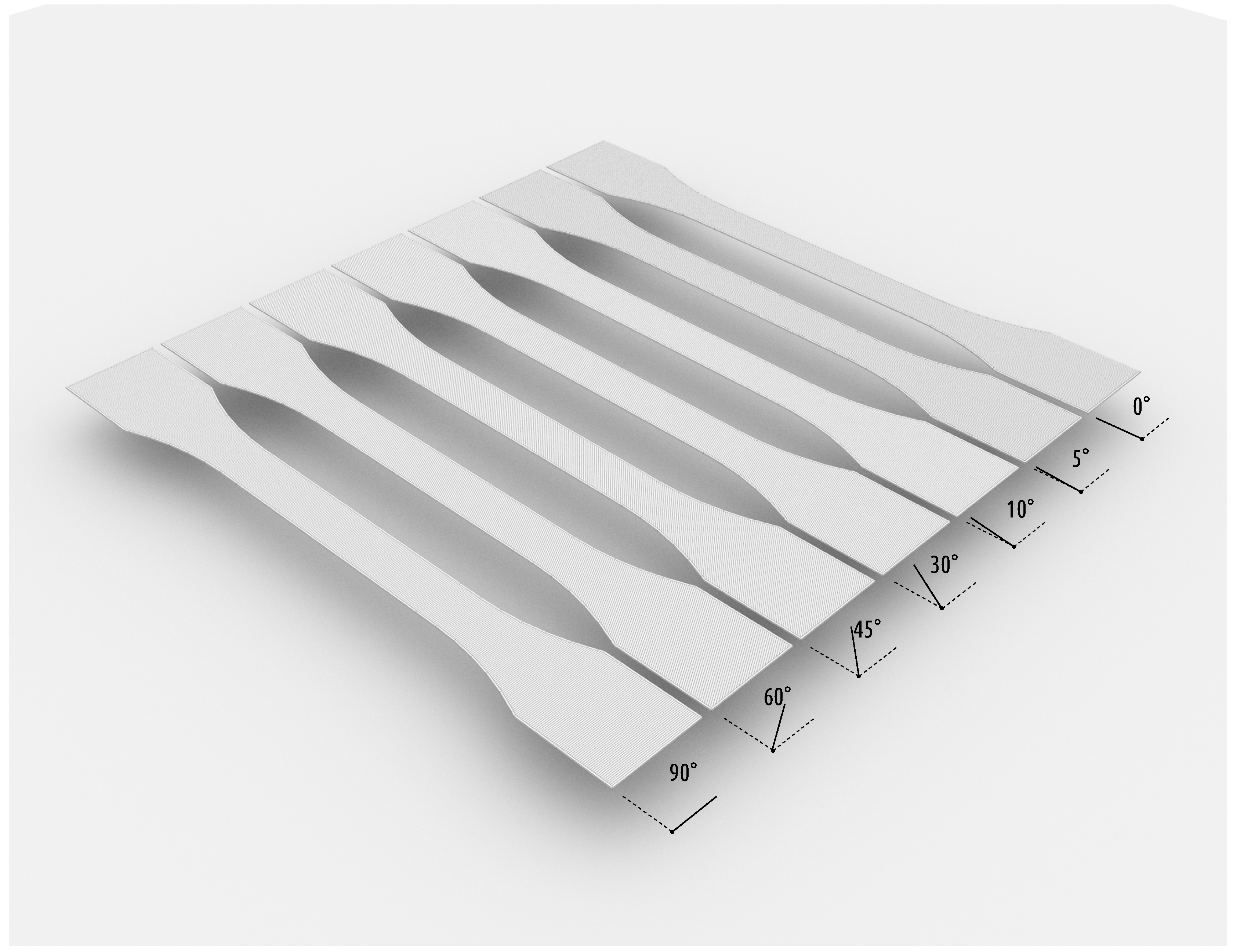
- Aligned, Mirrored second layer (flip)
- Aligned, Identical second layer (norm)
- Not Aligned (orient), Mirrored second layer (flip)
- Not Aligned (orient), Identical second layer (norm)
- 1 × 45 degrees norm orient, omitted due to machine error
- 3 × 10 degrees flip orient, printed but of unusable quality due to printing errors
1.1. Accuracy
2. Materials and Methods
- Crop the original form to contain each individual printed object
- Foreach cropped area of interest around the object do
- (a)
- Transform the Red-Green-Blue (Color Coding) (RGB) image data to Hue-Saturation-Value (Color Coding) (HSV) for more resistant colour based object detection
- (b)
- Identify image background and measurement mesh (static) and subtract from image
- (c)
- Binarize image by thresholding with most common colour in image
- (d)
- Utilise OpenCV blob detection algorithm on result and select largest blob as candidate for object detection
- (e)
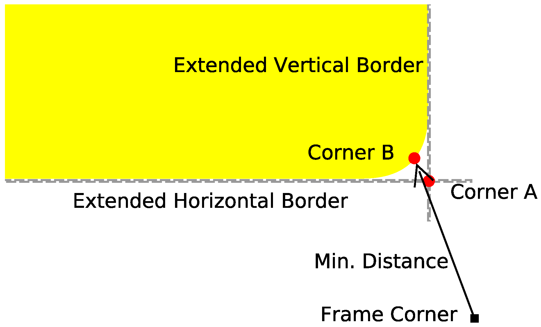
- Detect corners of object detection candidate and transform to array of line segments
- (f)
- Close holes within the maximum border segment
- (g)
- Create bounding-box around candidate object and compare to expected result
- if object candidate is verified then:
- Scan left side for corner top-left (Point A)
- Scan left side for corner bottom-left (Point B)
- Scan right side for corner top-right (Point C)
- Scan right side for corner bottom-right (Point D)
- Calculate distance between Point A and Point C (Distance Top) and angle against horizontal for AC
- Calculate distance between Point B and D (Distance Bottom) and angle against horizontal for BD
- Calculate distance between Point A and B (Distance Left) and angle against horizontal for AB
- Calculate distance between Point C and D (Distance Right) and angle against horizontal for CD
- Determine average X position of upper border near object centre
- Determine average X position of lower border near object center
- Calculate Average distance between upper and lower border near object centre (Middle Width)
- Calculate area surrounded by detected border divided by area of bounding box
- (h)
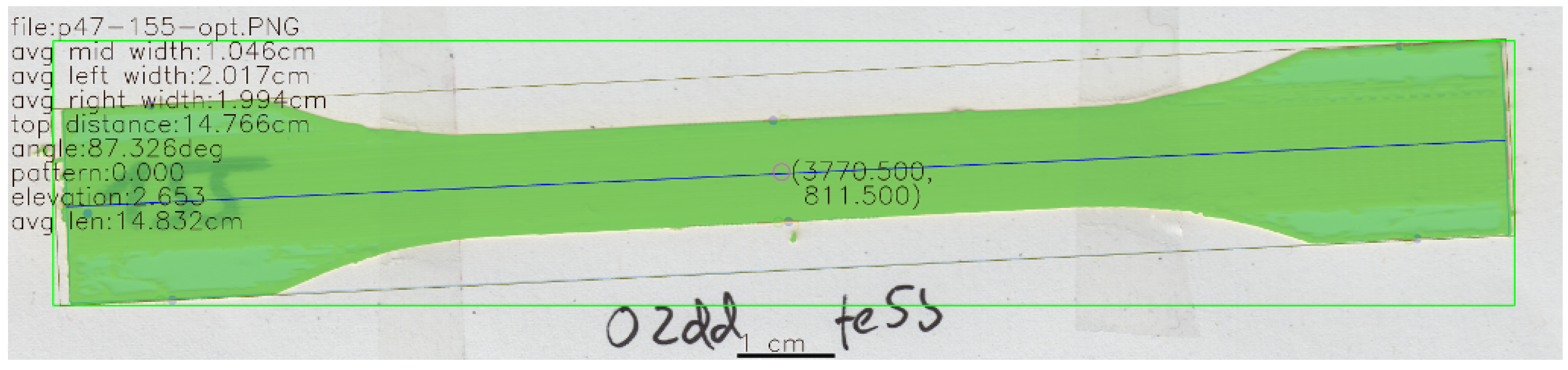
- Create overlay information for original image (intended for human usage)
- (i)
- Store data in database for later retrieval
2.1. Error Estimation
- max and min for the maximum and minimum measured distances for the 1 cm reference in pixels (pxs)
- pos. diff and neg. diff for the positive and negative difference to the theoretical value for the reference distance as indicated in Table 4.
- pos. diff % and neg. diff % for the percentage difference of the differences to the theoretical values
- pos. diff real and neg. diff real for the real-world differences in mm to the theoretical value.
2.2. On the Data Acquisition Device and Data Acquisition
3. Dataset Description
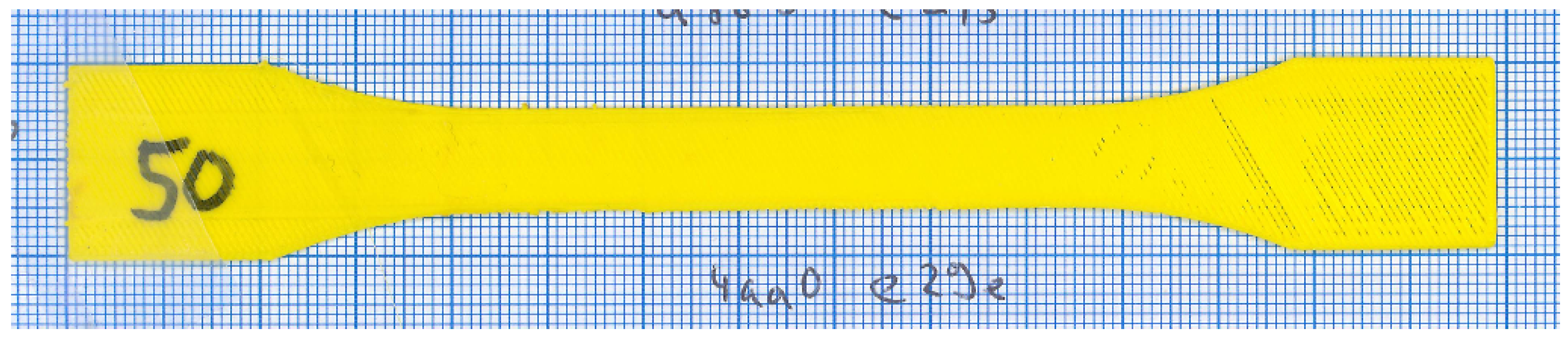
- Part A, contains the original scanned A4 papers with the specimens affixed.
- Part B, contains the cropped and extracted, unaltered scanned data for each individual specimen.
- Part C, contains the augmented image data for each individual specimen as provided by the analysis software.
- Part D, contains the data files for each individual specimen as provided by the analysis software.
- Width - Width of the scanned image in pixel (px) (7440)
- Height - Height of the scanned image in pixel (px) (1648)
- h - Colour Hue in the Hue-Saturation-Value (Color Coding) (HSV) Colourspace of the most dominant colour (25)
- s - Colour Saturation in the HSV Colourspace of the most dominant colour (165)
- v - Colour Value in the HSV Colourspace of the most dominant colour (247)
- r - Colour Value Red-Channel in the Red-Green-Blue (Color Coding) (RGB) Colourspace of the most dominant colour (88)
- g - Colour Value Green-Channel in the RGB Colourspace of the most dominant colour (218)
- b - Colour Value Blue-Channel in the RGB Colourspace of the most dominant colour (247)
- cm_factor - Factor to calculate from pixels to cm (236.22047)
- tmp_area - Largest found area for further detection (4908256.00000)
- calc_dist_right_side - Calculated distance at the right side (width) in pixel (px) (984.67546)
- calc_dist_right_side_cm - Calculated distance at the right side (width) in cm (2.08423)
- avg_right_side_A_x - Average X position for point A for the distance calculation (6718.12857)
- avg_right_side_A_Y - Average Y position for point A for the distance calculation (1122.64286)
- avg_right_side_B_X - Average Y position for point B for the distance calculation (6722.41860)
- avg_right_side_B_Y - Average Y position for point B for the distance calculation (137.97674)
- line_1_right_side - Definition of a line through the positions of elements detected on the border of the right top side in the form of . Gradient and y-intercept (−0.04906 + 1452.20479)
- line_2_right_side - Definition of a line through the positions of elements detected on the border of the right bottom side in the form of . Gradient and y-intercept (−0.04322 + 428.53713)
- distA_right_side - Calculated distance of a line perpendicular to the line_1_right_side and its intersection of line_2_right_side in pixel (px) (983.28993)
- distA_right_side_cm - Calculated distance of a line perpendicular to the line_1_right_side and its intersection of line_2_right_side in cm (2.08130)
- distB_right_side - Calculated distance of a line perpendicular to the line_2_right_side and its intersection of line_1_right_side in pixel (px) (983.57903)
- distB_right_side_cm - Calculated distance of a line perpendicular to the line_2_right_side and its intersection of line_1_right_side in cm (2.08191)
- distAB_right_side_avg - Average of distA_right_side and distB_right_side in pixel (px) (983.43448)
- distAB_right_side_avg_cm - Average of distA_right_side_cm and distB_right_side_cm in cm (2.08160)
- calc_dist_left_side - Calculated distance between the the points defined by avg_right_side_A_x, avg_right_side_A_y and avg_right_side_B_x, avg_right_side_B_y in pixel (px) (981.34574)
- calc_dist_left_side - Calculated distance between the the points defined by avg_right_side_A_x, avg_right_side_A_y and avg_right_side_B_x, avg_right_side_B_y in cm (2.07718)
- avg_left_side_A_x - Analogue to avg_right_side_A_x but for the left side of the specimen (690.45745)
- avg_left_side_A_y - Analogue to avg_right_side_A_y but for the left side of the specimen (1399.79787)
- avg_left_side_B_x - Analogue to avg_right_side_B_x but for the left side of the specimen (606.27723)
- avg_left_side_B_y - Analogue to avg_right_side_B_y but for the left side of the specimen (422.06931)
- line_1_left_side - Analogue to line_1_right_side but for the left side of the specimen (−0.04133 + 1428.33131)
- line_2_left_side - Analogue to line_1_right_side but for the left side of the specimen (−0.04113 + 447.00702)
- distA_left_side - Analogue to distA_right_side but for the left side of the specimen (980.37059)
- distA_left_side_cm - Analogue to distA_right_side_cm but for the left side of the specimen (2.07512)
- distB_left_side - Analogue to distB_right_side but for the left side of the specimen (980.36215)
- distB_left_side_cm - Analogue to distB_right_side_cm but for the left side of the specimen (2.07510)
- distAB_left_side_avg - Analogue to distAB_right_side_avg but for the left side of the specimen (980.36637)
- distAB_left_side_avg_cm - Analogue to distAB_left_side_avg_cm but for the left side of the specimen (2.07511)
- calc_dist_length - Analogue to calc_dist_right_side but for the length of the specimen (7029.23297)
- calc_dist_length_cm - Analogue to calc_dist_right_side_cm but for the length of the specimen (14.87854)
- avg_length_A_x - Analogue to avg_right_side_A_x but for the length of the specimen (170.87179)
- avg_length_A_y - Analogue to avg_right_side_A_y but for the length of the specimen (955.38462)
- avg_length_B_x - Analogue to avg_right_side_B_x but for the length of the specimen (7192.50000)
- avg_length_B_y - Analogue to avg_right_side_B_y but for the length of the specimen (628.50000)
- line_1_length - Analogue to line_1_right_side but for the length of the specimen (−0.87051 + 1104.13027)
- line_2_length - Analogue to line_2_right_side but for the length of the specimen (25.57616 + −183328.02318)
- distA_length - Analogue to distA_right_side but for the length of the specimen (6963.98400)
- distA_length_cm - Analogue to distA_right_side_cm but for the length of the specimen (14.74043)
- distB_length - Analogue to distB_right_side but for the length of the specimen (11217.47002)
- distB_length_cm - Analogue to distB_right_side_cm but for the length of the specimen (23.74364)
- distAB_length_avg - Analogue to distAB_right_side_avg but for the length of the specimen (7029.23297)
- distAB_length_avg_cm - Analogue to distAB_right_side_avg_cm but for the length of the specimen (14.87854)
- calc_dist_center - Analogue to calc_dist_right_side but for the centre width of the specimen (541.39512)
- calc_dist_center_cm - Analogue calc_dist_right_side_cm but for the centre width of the specimen (1.14595)
- avg_center_A_x - Analogue to avg_right_side_A_x but for the centre width of the specimen (3675.02713)
- avg_center_A_y - Analogue to avg_right_side_A_y but for the centre width of the specimen (1034.01938)
- avg_center_B_x - Analogue to avg_right_side_B_x but for the centre width of the specimen (3783.48889)
- avg_center_B_y - Analogue to avg_right_side_B_y but for the centre width of the specimen (503.60000)
- line_1_center - Analogue to line_1_right_side but for the centre width of the specimen (−0.04396 + 1195.57271)
- line_2_center - Analogue to line_2_right_side but for the centre width of the specimen (−0.05674 + 718.26909)
- distA_center - Analogue to distA_right_side but for the centre width of the specimen (525.18692)
- distA_center_cm - Analogue to distA_right_side_cm but for the centre width of the specimen (1.11165)
- distB_center - Analogue to distB_right_side but for the centre width of the specimen (523.46612)
- distB_center_cm - Analogue to distB_right_side_cm but for the centre width of the specimen (1.10800)
- distAB_center_avg - Analogue to distAB_right_side_avg but for the centre width of the specimen (524.32652)
- distAB_center_avg_cm - Analogue to distAB_right_side_avg_cm but for the centre width of the specimen (1.10982)
- end area_index - Index within the internal structure of found objects for software debugging (15)
- angle avg - The infill pattern detected in degrees. Detected by converting a portion around the centroid to binary and edge detection on the binarized image. The detected edges are averaged over all detected edges in the area of 120 pixel (px) height and width (41.50000)
- rotated rect extent - Extent as described above but for the rotated bounding box, is always 1 (1.00000)
- rotated rect len - The length of the rotated bounding box in px (16096.83508)
- rotated rect area - The area of the rotated bounding box in square px (7036683.00000)
- center x - X Position of the center point (3682.09366)
- center y - Y Position of the center point (772.77529)
- file - Full file name of scanned data (/mnt/experiment/sXX-67-opt.png)
- corner left top - Position of the top-left corner as X and Y coordinates (176,449)
- corner right top - Position of the top-left corner as X and Y coordinates (7168,158)
- corner left bot - Position of the top-left corner as X and Y coordinates (211,1419)
- corner right bot - Position of the top-left corner as X and Y coordinates (7197,1101)
- top distance px - Calculated distance between the bottom corners in pixel (px) (6998.05294)
- top distance cm - Calculated distance between the bottom corners in cm (14.81255)
- bot distance px - Calculated distance between the bottom corners in pixel (px) (6993.23387)
- bot distance cm - Calculated distance between the bottom corners in cm (14.80235)
- elevation - Internal parameter of the enclosing ellipse, elevation of ellipse (−0.04162)
- m_middle - Internal parameter of the enclosing ellipse (0.04357)
- m_angle - Internal parameter of the enclosing ellipse (2.49471)
- contour_perimeter - Length of the contour around the detected object in pixel (px) (17065.90852)
- contour_perimeter_adj - Length of the contour around the detected object adjusted by the cm_factor to make it comparable among scanned files with differing resolution (36.12284)
- extent - The extent of the detected object which is defined by the ratio of the contour area to the bounding box area (0.70249)
- solid - The solidity of the detected object which is defined by the ratio of the contour area to its convex hull area (0.53456)
- angle - Angle of the detected infill pattern (87.17921)
- bounding box (x, y, w, h) - X and Y position of the top left corner for the bounding box with the width and height of the bounding box (156, 125, 7057, 1301)
- bounding box area px - Area of the bounding box for the object in square cm (4907847.50000)
- processing_time - Processing time for the geometry extraction in s (2.93760)
4. Summary
5. Usage Notes
6. Concluding Remarks
7. Dataset Availability
Acknowledgments
Author Contributions
Conflicts of Interest
Abbreviations
| 3DP | 3D Printing (Technology) |
| ABS | Acrylonitrile butadiene styrene |
| AM | Additive Manufacturing |
| AMF | Advance Manufacturing Format |
| CIS | Contact Image Sensor |
| CT | Computer Tomography |
| DPI | Dots per Inch |
| FDM | Fused Deposition Modeling |
| FFF | Fused Filament Fabrication |
| HSV | Hue-Saturation-Value (Color Coding) |
| LOM | Laminated Object Modeling |
| LZW | Lempel-Ziv-Welch (Algorithm) |
| MiB | Mebibyte |
| PLA | Polylactic Acid |
| PNG | Portable Network Graphics (File Format) |
| RGB | Red-Green-Blue (Color Coding) |
| RM | Rapid Manufacturing |
| RP | Rapid Prototyping |
| RT | Rapid Tooling |
| SLA | Stereolithography |
| SLM | Selective Laser Melting |
| SLS | Selective Laser Sintering |
| STL | Stereolithography (File Format) |
| TIFF | Tagged Image File Format |
| px | Pixel |
References
- Gibson, I.; Rosen, D.; Stucker, B. Additive Manufacturing Technologies, 2nd ed.; Springer: New York, NY, USA, 2015. [Google Scholar]
- Wong, K.V.; Hernandez, A. A Review of Additive Manufacturing. ISRN Mech. Eng. 2012, 2012, 1–10. [Google Scholar] [CrossRef]
- Turner, B.N.; Strong, R.; Gold, S.A. A review of melt extrusion additive manufacturing processes: I. Process design and modeling. Rapid Prototyp. J. 2014, 20, 192–204. [Google Scholar] [CrossRef]
- Mohamed, O.A.; Masood, S.H.; Bhowmik, J.L. Optimization of fused deposition modeling process parameters: A review of current research and future prospects. Adv. Manuf. 2015, 3, 42–53. [Google Scholar] [CrossRef]
- ISO. 6983-1:2009 Automation Systems and Integration–Numerical Control of Machines—Program Format and Definitions of Address Words; International Organization for Standardization: Geneva, Switzerland, 2009. [Google Scholar]
- ASTM ISO. ASTM52915-13, Standard Specification for Additive Manufacturing File Format (AMF) Version 1.1; ASTM_International: West Conshohocken, PA, USA, 2013. [Google Scholar]
- Baumann, F.; Roller, D. 3D Printing Process Pipeline on the Internet. In Proceedings of the 8th ZEUS Workshop, Vienna, Austria, 27–28 January 2016; pp. 29–36.
- Bonten, C. Kunststofftechnik; Carl Hanser Verlag GmbH & Co. KG: Munich, Germany, 2014. [Google Scholar]
- Nuñez, P.J.; Rivas, A.; García-Plaza, E.; Beamud, E.; Sanz-Lobera, A. Dimensional and Surface Texture Characterization in Fused Deposition Modelling (FDM) with ABS plus—In MESIC Manufacturing Engineering Society International Conference 2015. Procedia Eng. 2015, 132, 856–863. [Google Scholar] [CrossRef]
- Baumann, F.; Schön, M.; Roller, D. Concept Development of a Sensor Array for 3D Printer. In Proceeding of the 3rd International Conference on Ramp Up Management (ICRM 2016), Aachen, Germany, 22–24 June 2016.
- Ippolito, R.; Iuliano, L.; Gatto, A. Benchmarking of Rapid Prototyping Techniques in Terms of Dimensional Accuracy and Surface Finish. CIRP Ann.-Manuf. Technol. 1995, 44, 157–160. [Google Scholar] [CrossRef]
- Fadel, G.M.; Kirschman, C. Accuracy issues in CAD to RP translations. Rapid Prototyp. J. 1996, 2, 4–17. [Google Scholar] [CrossRef]
- Pham, D.T.; Gault, R.S. A comparison of rapid prototyping technologies. Int. J. Mach. Tools Manuf. 1998, 38, 1257–1287. [Google Scholar] [CrossRef]
- Matta, A.K.; Raju, D.R.; Suman, K.N.S. The Integration of CAD/CAM and Rapid Prototyping in Product Development: A Review—In 4th International Conference on Materials Processing and Characterzation. Mater. Today Proc. 2015, 2, 3438–3445. [Google Scholar] [CrossRef]
- Bikas, H.; Stavropoulos, P.; Chryssolouris, G. Additive manufacturing methods and modelling approaches: A critical review. Int. J. Adv. Manuf. Technol. 2016, 83, 389–405. [Google Scholar] [CrossRef]
- Boparai, K.S.; Singh, R.; Singh, H. Development of rapid tooling using fused deposition modeling: A review. Rapid Prototyp. J. 2016, 22, 281–299. [Google Scholar] [CrossRef]
- Dimitrov, D.; van Wijck, W.; Schreve, K.; de Beer, N. Investigating the achievable accuracy of three dimensional printing. Rapid Prototyp. J. 2006, 12, 42–52. [Google Scholar] [CrossRef]
- Turner, B.N.; Gold, S.A. A review of melt extrusion additive manufacturing processes: II. Materials, dimensional accuracy, and surface roughness. Rapid Prototyp. J. 2015, 21, 250–261. [Google Scholar] [CrossRef]
- Boschetto, A.; Bottini, L. Accuracy prediction in fused deposition modeling. Int. J. Adv. Manuf. Technol. 2014, 73, 913–928. [Google Scholar] [CrossRef]
- Armillotta, A. Assessment of surface quality on textured FDM prototypes. Rapid Prototyp. J. 2006, 12, 35–41. [Google Scholar] [CrossRef]
- Equbal, A.; Sood, A.K.; Mahapatra, S.S. Prediction of dimensional accuracy in fused deposition modelling: A fuzzy logic approach. Int. J. Prod. Qual. Manag. 2011, 7, 22–43. [Google Scholar] [CrossRef]
- Sahu, R.K.; Mahapatra, S.S.; Sood, A.K. A Study on Dimensional Accuracy of Fused Deposition Modeling (FDM) Processed Parts using Fuzzy Logic. J. Manuf. Sci. Prod. 2013, 13, 183–197. [Google Scholar] [CrossRef]
- Masood, S.H.; Morsi, Y.S.; Katatny, I.E. Evaluation and Validation of the Shape Accuracy of FDM Fabricated Medical Models. Adv. Mater. Res. 2010, 83, 275–280. [Google Scholar]
- Tong, K.; Joshi, S.; Lehtihet, E.A. Error compensation for fused deposition modeling (FDM) machine by correcting slice files. Rapid Prototyp. J. 2008, 14, 4–14. [Google Scholar] [CrossRef]
- Boschetto, A.; Bottini, L. Design for manufacturing of surfaces to improve accuracy in Fused Deposition Modeling. Rob. Comput.-Integr. Manuf. 2016, 37, 103–114. [Google Scholar] [CrossRef]
- Garg, A.; Bhattacharya, A.; Batish, A. On Surface Finish and Dimensional Accuracy of FDM Parts after Cold Vapor Treatment. Mater. Manuf. Process. 2016, 31, 522–529. [Google Scholar] [CrossRef]
- MITUTOYO|Product Information. Available online: https://www.mitutoyo.co.jp/eng/products/nogisu/hyojyun.html (accessed on 20 January 2016).
- Taylor Hobson–Surface Profilers|Surface Profiliometer. Available online: http://www.taylor-hobson.com (accessed on 20 January 2016).
- Canon CanoScan LiDE 90 – Canon Europe. Available online: www.canon-europe.com/support/ consumer_products/products/scanners/lide_series/canoscan_lide_90.aspx (accessed on 20 January 2016).
- LTF – Prodotti Trovati. Available online: http://www.ltf.it/en/prodotti_lista.php (accessed on 20 January 2016).
- Technical Support for Picza LPX-250RE 3D Laser Scanner. Available online: http://support.rolanddga.com/_layouts/rolanddga/productdetail.aspx?pm=LPX-250 (accessed on 20 January 2016).
- AG, C.Z. ZEISS Industrial Metrology Homepage. Available online: www.zeiss.com/metrology/home.html (accessed on 20 January 2016).
- Nikon Metrology, I. Optical Comparators|Video & Microscope Measuring|Products|Nikon Metrology. Available online: http://www.nikonmetrology.com/Products/Video-Microscope-Measuring/Optical-Comparators (accessed on 20 January 2016).
- ISO. Information Technology–Computer Graphics and Image Processing–Portable Network Graphics (PNG): Functional Specification; ISO ISO/IEC 15948:2004; International Organization for Standardization: Geneva, Switzerland, 2004. [Google Scholar]
- Dheemanth, H.N. LZW Data Compression. Am. J. Eng. Res. 2014, 3, 22–26. [Google Scholar]
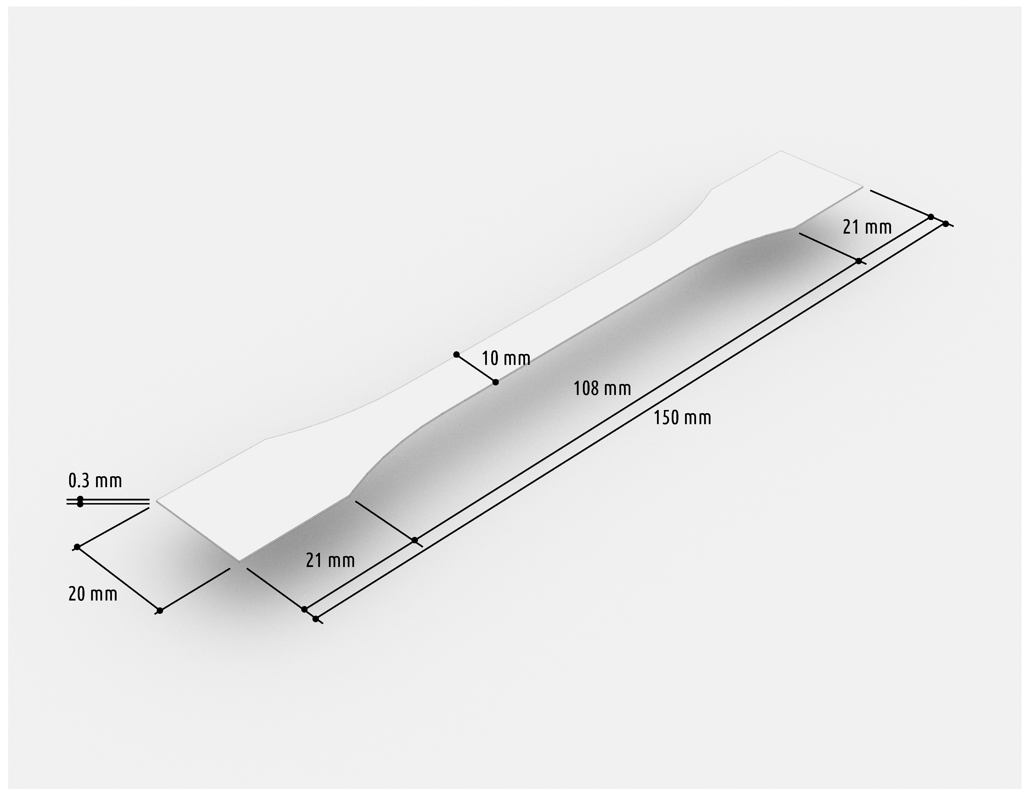
- DIN EN ISO. 527-2:2012-06 – Kunststoffe - Bestimmung der Zugeigenschaften - Teil 2: Prüfbedingungen für Form-und Extrusionsmassen (ISO 527-2:2012); ISO: Geneva, Switzerland, 2012. (In Germany) [Google Scholar]
- Baumann, F.W.; Wellekötter, J.; Roller, D.; Bonten, C. Software-aided measurement of geometrical fidelity for 3D printed objects. Comput.-Aid. Des. Appl. 2016, 1–12. [Google Scholar] [CrossRef]


| Source | Achieved Accuracy | Applied for | Applicable for | Restriction(s) | Type |
|---|---|---|---|---|---|
| [21] | 0.01 mm | Fused Deposition Modeling (FDM) | 3D-objects | None | Manual – Using Mitutoyo [27] Vernier Calliper |
| [22] | 0.01 mm | FDM | 3D-objects | None | Manual – Using Mitutoyo [27] Vernier Calliper |
| [19] | 16 nm | FDM | Surface profile of planar 3D-objects | FDM | Manual – Using Taylor Hobson Form Talyprofile Plus [28] |
| [25] | 0.22 mm | FDM | 3D-objects with planar surface | None | Image processing – Canon Canoscan Lide 90 [29] 1200 dpi, and manual measurement with Borletti MEL/N 2W [30] micrometer |
| [18] | N/A | None | Various | None | Theoretical, Review |
| [23] | 0.2 mm | FDM | 3D-objects | None | Laser-Scanning – Using Roland LPX-250 [31] |
| [24] | N/A | FDM+ Stereolithography (SLA) | 3D-objects | None | Carl Zeiss ECLIPSE 550 CMM [32] |
| [26] | 0.001 mm | FDM+ surface treatment | 3D-objects | None | Manual – Using Mitutoyo SJ400 [27] for surface roughness, dimensions with Nikon V-10A [33] |
| dpi | Max. Equivalent of 1 Pixel (px) in mm | Number of Available Images | Avg. Filesize in MiB | Average Image Width in Pixel (px) | Average Image Height in Pixel (px) |
|---|---|---|---|---|---|
| 600 | 0.0423333 | 17 | 47.0928 | 4997.4705 | 5410.8235 |
| 1200 | 0.0211666 | 21 | 180.3056 | 10,224.0000 | 10,893.2857 |
| 2400 | 0.0105833 | 19 | 688.6836 | 20,464.0000 | 21,943.4736 |
| 4800 | 0.0052916 | 13 | 1323.7478 | 40,944.0000 | 45,268.6153 |
| dpi | max | min | pos. diff | neg. diff | pos. diff % | neg. diff % | pos. diff real | neg. diff real |
|---|---|---|---|---|---|---|---|---|
| 600 | 246 | 228 | 9.78 | −8.22 | 4.14 % | 3.48 % | 0.41 mm | −0.35 mm |
| 1200 | 493 | 458 | 20.56 | −14.44 | 4.35 % | 3.06 % | 0.44 mm | −0.31 mm |
| 2400 | 984 | 917 | 39.12 | −27.88 | 4.14 % | −2.95 % | 0.41 mm | −0.30 mm |
| 4800 | 1952 | 1827 | 62.21 | −62.79 | 3.29 % | −3.32 % | 0.33 mm | −0.33 mm |
| 1 px equiv. × mm | 1 cm equiv. × px | |
|---|---|---|
| 600 | 0.0423333 | 236.22 |
| 1200 | 0.0211666 | 472.44 |
| 2400 | 0.0105833 | 944.88 |
| 4800 | 0.0052916 | 1889.79 |
| dpi | Average | diff | diff % | diff Real |
|---|---|---|---|---|
| 600 | 237.0 | 0.78 | 0.33 % | 0.033 mm |
| 1200 | 475.5 | 3.06 | 0.65 % | 0.065 mm |
| 2400 | 950.5 | 5.62 | 0.59 % | 0.059 mm |
| 4800 | 1889.5 | −0.29 | 0.02 % | 0.002 mm |
| # | Page | Specimen # | Filename | Filesize in Bytes | Resolution in dpi | Image Width in Pixel (px) | Image Height in Pixel (px) |
|---|---|---|---|---|---|---|---|
| 0 | 27 | 1 | p27-1-1200.PNG | 15,802,136 | 1200 | 7567 | 1495 |
| 1 | 27 | 1 | p27-1-600.PNG | 4,283,824 | 600 | 3685 | 759 |
| 2 | 27 | 2 | p27-2-1200.PNG | 16,257,137 | 1200 | 7429 | 1656 |
| 3 | 27 | 2 | p27-2-600.PNG | 4,213,422 | 600 | 3696 | 792 |
| 4 | 27 | 3 | p27-3-1200.PNG | 17,487,534 | 1200 | 7728 | 1725 |
| 5 | 27 | 3 | p27-3-600.PNG | 4,085,988 | 600 | 3596 | 768 |
| 6 | 27 | 4 | p27-4-1200.PNG | 18,594,572 | 1200 | 7429 | 1932 |
| 7 | 27 | 4 | p27-4-600.PNG | 3,425,931 | 600 | 3632 | 672 |
| 8 | 27 | 5 | p27-5-1200.PNG | 18,471,306 | 1200 | 7544 | 1863 |
| 9 | 27 | 5 | p27-5-600.PNG | 4,214,080 | 600 | 3632 | 804 |
| 10 | 27 | 6 | p27-6-1200.PNG | 15,456,270 | 1200 | 7452 | 1587 |
| 11 | 27 | 6 | p27-6-600.PNG | 3,405,681 | 600 | 3652 | 668 |
| 12 | 27 | 7 | p27-7-1200.PNG | 17,927,279 | 1200 | 7705 | 1725 |
| 13 | 27 | 7 | p27-7-600.PNG | 3,381,149 | 600 | 3628 | 672 |
| 14 | 28 | 10 | p28-10-1200.PNG | 18,385,665 | 1200 | 7613 | 1863 |
| 15 | 28 | 10 | p28-10-600.PNG | 3,795,305 | 600 | 3636 | 748 |
| 16 | 28 | 11 | p28-11-1200.PNG | 15,190,521 | 1200 | 7406 | 1541 |
| 17 | 28 | 11 | p28-11-600.PNG | 3,505,724 | 600 | 3646 | 660 |
| 18 | 28 | 12 | p28-12-1200.PNG | 15,950,936 | 1200 | 7291 | 1633 |
| 19 | 28 | 12 | p28-12-600.PNG | 3,426,744 | 600 | 3625 | 671 |
| 20 | 28 | 13 | p28-13-1200.PNG | 15,936,818 | 1200 | 7544 | 1587 |
| 21 | 28 | 13 | p28-13-600.PNG | 4,649,833 | 600 | 3624 | 852 |
| 22 | 28 | 14 | p28-14-1200.PNG | 16,473,597 | 1200 | 7636 | 1564 |
| 23 | 28 | 14 | p28-14-600.PNG | 3,950,749 | 600 | 3658 | 737 |
| 24 | 28 | 8 | p28-8-1200.PNG | 17,216,974 | 1200 | 7360 | 1794 |
| 25 | 28 | 8 | p28-8-600.PNG | 4,600,434 | 600 | 3773 | 858 |
| 26 | 28 | 9 | p28-9-1200.PNG | 16,645,140 | 1200 | 7590 | 1702 |
| 27 | 28 | 9 | p28-9-600.PNG | 33,88,757 | 600 | 3685 | 693 |
| 28 | 29 | 15 | p29-15-1200.PNG | 13,875,443 | 1200 | 7383 | 1449 |
| 29 | 29 | 16 | p29-16-1200.PNG | 15,349,450 | 1200 | 7475 | 1587 |
| 30 | 29 | 17 | p29-17-1200.PNG | 16,837,443 | 1200 | 7544 | 1725 |
| 31 | 29 | 18 | p29-18-1200.PNG | 15,908,333 | 1200 | 7406 | 1656 |
| 32 | 29 | 19 | p29-19-1200.PNG | 14,721,827 | 1200 | 7337 | 1541 |
| 33 | 29 | 20 | p29-20-1200.PNG | 16,315,248 | 1200 | 7452 | 1656 |
| 34 | 30 | 21 | p30-21-1200.PNG | 20,695,527 | 1200 | 7728 | 1978 |
| 35 | 30 | 22 | p30-22-1200.PNG | 17,279,097 | 1200 | 7475 | 1725 |
| 36 | 30 | 22 | p30-22-600.PNG | 4,152,746 | 600 | 3795 | 792 |
| 37 | 30 | 23 | p30-23-1200.PNG | 17,717,957 | 1200 | 7475 | 1748 |
| 38 | 30 | 24 | p30-24-1200.PNG | 15,798,242 | 1200 | 7636 | 1518 |
| 39 | 30 | 25 | p30-25-1200.PNG | 15,247,463 | 1200 | 7268 | 1541 |
| 40 | 30 | 26 | p30-26-1200.PNG | 15,821,651 | 1200 | 7452 | 1541 |
| 41 | 30 | 27 | p30-27-1200.PNG | 16,893,003 | 1200 | 7567 | 1587 |
| 42 | 31 | 28 | p31-28-1200.PNG | 12,403,406 | 1200 | 7326 | 1320 |
| 43 | 31 | 29 | p31-29-1200.PNG | 13,687,842 | 1200 | 7326 | 1430 |
| 44 | 31 | 31 | p31-31-1200.PNG | 13,380,146 | 1200 | 7238 | 1419 |
| 45 | 31 | 32 | p31-32-1200.PNG | 15,916,530 | 1200 | 7194 | 1672 |
| 46 | 32 | 36 | p32-36-1200.PNG | 22,134,196 | 1200 | 7728 | 2185 |
| 47 | 32 | 39 | p32-39-1200.PNG | 16,769,168 | 1200 | 7567 | 1702 |
| 48 | 34 | 47 | p34-47-1200.PNG | 17,601,188 | 1200 | 7475 | 1725 |
| 49 | 34 | 47 | p34-47-600.PNG | 4,951,121 | 600 | 3718 | 825 |
| 50 | 34 | 48 | p34-48-1200.PNG | 19,140,905 | 1200 | 7567 | 1886 |
| 51 | 34 | 48 | p34-48-600.PNG | 5,254,171 | 600 | 3740 | 814 |
| 52 | 34 | 49 | p34-49-1200.PNG | 14,877,228 | 1200 | 7337 | 1541 |
| 53 | 34 | 49 | p34-49-600.PNG | 4,659,681 | 600 | 3674 | 759 |
| 54 | 34 | 50 | p34-50-1200.PNG | 15,902,008 | 1200 | 7797 | 1541 |
| 55 | 34 | 50 | p34-50-600.PNG | 4,940,355 | 600 | 3795 | 781 |
| 56 | 34 | 51 | p34-51-1200.PNG | 18,265,770 | 1200 | 7498 | 1817 |
| 57 | 34 | 51 | p34-51-600.PNG | 5,664,148 | 600 | 3685 | 891 |
| 58 | 35 | 52 | p35-52-1200.PNG | 17,277,241 | 1200 | 7314 | 1794 |
| 59 | 35 | 53 | p35-53-1200.PNG | 16,928,700 | 1200 | 7291 | 1725 |
| 60 | 35 | 54 | p35-54-1200.PNG | 17,813,955 | 1200 | 7521 | 1771 |
| 61 | 35 | 55 | p35-55-1200.PNG | 15,224,841 | 1200 | 7406 | 1587 |
| 62 | 35 | 56 | p35-56-1200.PNG | 14,129,557 | 1200 | 7314 | 1495 |
| 63 | 35 | 57 | p35-57-1200.PNG | 14,474,452 | 1200 | 7498 | 1472 |
| 64 | 36 | 59 | p36-59-1200.PNG | 15,888,111 | 1200 | 8248 | 1616 |
| 65 | 36 | 60 | p36-60-1200.PNG | 12,207,369 | 1200 | 7264 | 1416 |
| 66 | 36 | 61 | p36-61-1200.PNG | 12,231,145 | 1200 | 7216 | 1400 |
| 67 | 36 | 62 | p36-62-1200.PNG | 11,898,430 | 1200 | 7248 | 1376 |
| 68 | 36 | 63 | p36-63-1200.PNG | 10,812,265 | 1200 | 7208 | 1248 |
| 69 | 36 | 64 | p36-64-1200.PNG | 13,461,738 | 1200 | 7336 | 1528 |
| 70 | 36 | 65 | p36-65-1200.PNG | 13,101,484 | 1200 | 7304 | 1474 |
| 71 | 36 | 66 | p36-66-1200.PNG | 12,640,867 | 1200 | 7370 | 1386 |
| 72 | 36 | 67 | p36-67-1200.PNG | 18,234,875 | 1200 | 7440 | 1648 |
| 73 | 36-b | 58 | p36-b-58-2400.PNG | 51,724,257 | 2400 | 14760 | 2925 |
| 74 | 36-b | 58 | p36-b-58-4800.PNG | 25,5270,856 | 4800 | 29520 | 5850 |
| 75 | 36-b | 58 | p36-b-58-600.PNG | 764,250 | 600 | 3768 | 792 |
| 76 | 36-b | 68 | p36-b-68-2400.PNG | 58,277,245 | 2400 | 15165 | 3195 |
| 77 | 36-b | 68 | p36-b-68-4800.PNG | 289,659,569 | 4800 | 30330 | 6390 |
| 78 | 36-b | 68 | p36-b-68-600.PNG | 969,708 | 600 | 3736 | 720 |
| 79 | 36-b | 69 | p36-b-69-2400.PNG | 61,167,921 | 2400 | 15120 | 3375 |
| 80 | 36-b | 69 | p36-b-69-4800.PNG | 121,977,342 | 4800 | 30240 | 6750 |
| 81 | 36-b | 69 | p36-b-69-600.PNG | 1,002,549 | 600 | 3720 | 784 |
| 82 | 36-b | 70 | p36-b-70-2400.PNG | 57,790,560 | 2400 | 14715 | 3240 |
| 84 | 36-b | 70 | p36-b-70-600.PNG | 1,418,770 | 600 | 3696 | 784 |
| 85 | 36-b | 71 | p36-b-71-2400.PNG | 70,141,930 | 2400 | 15165 | 3870 |
| 87 | 36-b | 71 | p36-b-71-600.PNG | 903,541 | 600 | 3760 | 856 |
| 88 | 36-b | 74 | p36-b-74-2400.PNG | 65,731,968 | 2400 | 15165 | 3555 |
| 90 | 36-b | 74 | p36-b-74-600.PNG | 694,650 | 600 | 3704 | 800 |
| 91 | 37 | 75 | p37-75-1200.PNG | 16,789,946 | 1200 | 7521 | 1748 |
| 92 | 37 | 76 | p37-76-1200.PNG | 17,901,974 | 1200 | 7567 | 1886 |
| 93 | 37 | 77 | p37-77-1200.PNG | 13,748,061 | 1200 | 7383 | 1541 |
| 94 | 37 | 78 | p37-78-1200.PNG | 13,234,855 | 1200 | 7344 | 1488 |
| 95 | 37 | 79 | p37-79-1200.PNG | 13,518,732 | 1200 | 7408 | 1504 |
| 96 | 37 | 80 | p37-80-1200.PNG | 12,801,393 | 1200 | 7280 | 1440 |
| 97 | 37 | 81 | p37-81-1200.PNG | 13,856,233 | 1200 | 7344 | 1536 |
| 98 | 39 | 82 | p39-82-1200.PNG | 12,347,713 | 1200 | 7336 | 1360 |
| 99 | 39 | 83 | p39-83-1200.PNG | 11,992,064 | 1200 | 7288 | 1336 |
| 100 | 39 | 84 | p39-84-1200.PNG | 12,403,777 | 1200 | 7304 | 1392 |
| 101 | 39 | 85 | p39-85-1200.PNG | 12,825,914 | 1200 | 7376 | 1432 |
| 102 | 39 | 86 | p39-86-1200.PNG | 11,931,825 | 1200 | 7248 | 1352 |
| 103 | 39 | 87 | p39-87-1200.PNG | 12,522,546 | 1200 | 7168 | 1432 |
| 104 | 39 | 88 | p39-88-1200.PNG | 12,947,536 | 1200 | 7296 | 1440 |
| 105 | 40 | 89 | p40-89-1200.PNG | 15,188,761 | 1200 | 7498 | 1633 |
| 106 | 40 | 89 | p40-89-2400.PNG | 256,951,082 | 2400 | 15180 | 3496 |
| 107 | 40 | 90 | p40-90-1200.PNG | 14,157,006 | 1200 | 7282 | 1584 |
| 108 | 40 | 90 | p40-90-2400.PNG | 251,947,008 | 2400 | 14904 | 3496 |
| 109 | 40 | 91 | p40-91-1200.PNG | 14,281,697 | 1200 | 7260 | 1617 |
| 110 | 40 | 91 | p40-91-2400.PNG | 216,170,177 | 2400 | 14950 | 2990 |
| 111 | 40 | 92 | p40-92-1200.PNG | 13,946,621 | 1200 | 7249 | 1573 |
| 112 | 40 | 92 | p40-92-2400.PNG | 253,921,221 | 2400 | 15226 | 3450 |
| 113 | 40 | 93 | p40-93-1200.PNG | 13,320,929 | 1200 | 7238 | 1507 |
| 114 | 40 | 93 | p40-93-2400.PNG | 218,252,498 | 2400 | 14858 | 3036 |
| 115 | 40 | 94 | p40-94-1200.PNG | 14,266,965 | 1200 | 7293 | 1617 |
| 116 | 40 | 94 | p40-94-2400.PNG | 235,251,629 | 2400 | 14904 | 3266 |
| 117 | 40 | 95 | p40-95-1200.PNG | 14,442,902 | 1200 | 7348 | 1584 |
| 118 | 40 | 95 | p40-95-2400.PNG | 219,781,430 | 2400 | 14950 | 3036 |
| 119 | 41 | 100 | p41-100-1200.PNG | 13,213,145 | 1200 | 7370 | 1463 |
| 120 | 41 | 101 | p41-101-1200.PNG | 13,323,247 | 1200 | 7326 | 1474 |
| 121 | 41 | 102 | p41-102-1200.PNG | 13,527,017 | 1200 | 7315 | 1441 |
| 122 | 41 | 96 | p41-96-1200.PNG | 16,063,579 | 1200 | 7452 | 1771 |
| 123 | 41 | 97 | p41-97-1200.PNG | 16,517,917 | 1200 | 7429 | 1840 |
| 124 | 41 | 98 | p41-98-1200.PNG | 15,756,626 | 1200 | 7498 | 1748 |
| 125 | 41 | 99 | p41-99-1200.PNG | 14,660,149 | 1200 | 7406 | 1633 |
| 126 | 42 | 108 | p42-108-2400.PNG | 53,718,608 | 2400 | 14938 | 2992 |
| 127 | 42 | 109 | p42-109-2400.PNG | 54,466,318 | 2400 | 14894 | 3058 |
| 128 | 42 | 110 | p42-110-2400.PNG | 50,484,992 | 2400 | 14762 | 2860 |
| 129 | 42 | 111 | p42-111-2400.PNG | 56,011,807 | 2400 | 14586 | 3234 |
| 130 | 42 | 114 | p42-114-2400.PNG | 51,721,723 | 2400 | 14938 | 2926 |
| 131 | 42 | 117 | p42-117-2400.PNG | 48,238,820 | 2400 | 14718 | 2750 |
| 132 | 42 | 118 | p42-118-2400.PNG | 52,439,840 | 2400 | 14894 | 2948 |
| 133 | 42-a | 104 | p42-a-104-1200.PNG | 15,651,976 | 1200 | 7314 | 1656 |
| 134 | 42-a | 105 | p42-a-105-1200.PNG | 12,558,931 | 1200 | 7326 | 1397 |
| 135 | 42-a | 106 | p42-a-106-1200.PNG | 14,685,907 | 1200 | 7337 | 1584 |
| 136 | 42-a | 107 | p42-a-107-1200.PNG | 14,410,532 | 1200 | 7381 | 1540 |
| 137 | 43 | 119 | p43-119-1200.PNG | 15,112,558 | 1200 | 7360 | 1648 |
| 138 | 43 | 119 | p43-119-2400.PNG | 65,666,516 | 2400 | 14940 | 3690 |
| 139 | 43 | 119 | p43-119-600.PNG | 4,507,979 | 600 | 3850 | 869 |
| 140 | 43 | 120 | p43-120-1200.PNG | 13,527,108 | 1200 | 7288 | 1488 |
| 141 | 43 | 120 | p43-120-2400.PNG | 56,249,982 | 2400 | 14940 | 3150 |
| 142 | 43 | 120 | p43-120-600.PNG | 4,344,477 | 600 | 3696 | 880 |
| 143 | 43 | 121 | p43-121-1200.PNG | 12,108,927 | 1200 | 7288 | 1320 |
| 144 | 43 | 121 | p43-121-2400.PNG | 58,926,508 | 2400 | 14850 | 3330 |
| 145 | 43 | 121 | p43-121-600.PNG | 4,367,353 | 600 | 3773 | 869 |
| 146 | 43 | 122 | p43-122-1200.PNG | 12,052,518 | 1200 | 7392 | 1304 |
| 147 | 43 | 122 | p43-122-2400.PNG | 59,192,015 | 2400 | 14940 | 3330 |
| 148 | 43 | 122 | p43-122-600.PNG | 4,066,311 | 600 | 3729 | 814 |
| 149 | 43 | 124 | p43-124-1200.PNG | 13,076,273 | 1200 | 7280 | 1432 |
| 150 | 43 | 124 | p43-124-2400.PNG | 58,627,856 | 2400 | 15120 | 3240 |
| 151 | 43 | 124 | p43-124-600.PNG | 3,966,950 | 600 | 3718 | 803 |
| 152 | 43 | 126 | p43-126-1200.PNG | 13,476,698 | 1200 | 7320 | 1464 |
| 153 | 43 | 126 | p43-126-2400.PNG | 52,758,176 | 2400 | 14940 | 2925 |
| 154 | 43 | 126 | p43-126-600.PNG | 3,863,005 | 600 | 3795 | 759 |
| 155 | 43 | 127 | p43-127-1200.PNG | 12,857,843 | 1200 | 7328 | 1392 |
| 156 | 43 | 127 | p43-127-2400.PNG | 52,801,769 | 2400 | 14760 | 2970 |
| 157 | 43 | 127 | p43-127-600.PNG | 3,859,578 | 600 | 3751 | 770 |
| 158 | 45 | 142 | p45-142-1200.PNG | 16,394,947 | 1200 | 7544 | 1725 |
| 159 | 45 | 143 | p45-143-1200.PNG | 15,123,653 | 1200 | 7544 | 1587 |
| 160 | 45 | 144 | p45-144-1200.PNG | 15,093,669 | 1200 | 7498 | 1610 |
| 161 | 45 | 145 | p45-145-1200.PNG | 15,131,686 | 1200 | 7475 | 1610 |
| 162 | 45 | 146 | p45-146-1200.PNG | 15,904,074 | 1200 | 7659 | 1656 |
| 163 | 45 | 147 | p45-147-1200.PNG | 15,752,037 | 1200 | 7590 | 1656 |
| 164 | 45 | 148 | p45-148-1200.PNG | 16,846,784 | 1200 | 7613 | 1748 |
| 165 | 46 | 149 | p46-149-1200.PNG | 15,574,132 | 1200 | 7613 | 1610 |
| 166 | 46 | 150 | p46-150-1200.PNG | 15,281,620 | 1200 | 7590 | 1587 |
| 167 | 47 | 151 | p47-151-1200.PNG | 16,877,101 | 1200 | 7337 | 1863 |
| 168 | 47 | 152 | p47-152-1200.PNG | 14,001,437 | 1200 | 7491 | 1507 |
| 169 | 47 | 155 | p47-155-1200.PNG | 16,294,742 | 1200 | 7535 | 1716 |
| 170 | 50 | 171 | p50-171-1200.PNG | 16,061,329 | 1200 | 7498 | 1679 |
| 171 | 50 | 171 | p50-171-2400.PNG | 15,126,063 | 2400 | 15712 | 3583 |
| 172 | 50 | 173 | p50-173-1200.PNG | 15,414,649 | 1200 | 7498 | 1633 |
| 173 | 50 | 173 | p50-173-2400.PNG | 21,872,017 | 2400 | 15200 | 3144 |
| 174 | 50 | 176 | p50-176-1200.PNG | 15,237,904 | 1200 | 7475 | 1610 |
| 175 | 50 | 176 | p50-176-2400.PNG | 20,824,114 | 2400 | 14768 | 3144 |
| 176 | 50 | 180 | p50-180-1200.PNG | 13,818,923 | 1200 | 7498 | 1449 |
| 177 | 50 | 180 | p50-180-2400.PNG | 21,686,585 | 2400 | 15344 | 3071 |
| 178 | 50 | 181 | p50-181-1200.PNG | 15,041,539 | 1200 | 7774 | 1518 |
| 179 | 50 | 181 | p50-181-2400.PNG | 22,589,243 | 2400 | 15488 | 2925 |
| 180 | 51 | 182 | p51-182-1200.PNG | 16,710,584 | 1200 | 7475 | 1771 |
| 181 | 51 | 182 | p51-182-2400.PNG | 25,453,500 | 2400 | 15280 | 3144 |
| 182 | 51 | 183 | p51-183-1200.PNG | 15,383,101 | 1200 | 7475 | 1633 |
| 183 | 51 | 183 | p51-183-2400.PNG | 25,004,238 | 2400 | 15344 | 3144 |
| 184 | 51 | 183 | p51-183-4800.PNG | 82,642,045 | 4800 | 30848 | 6727 |
| 185 | 51 | 184 | p51-184-1200.PNG | 14,678,869 | 1200 | 7590 | 1541 |
| 186 | 51 | 184 | p51-184-4800.PNG | 72,257,123 | 4800 | 29536 | 5996 |
| 187 | 51 | 185 | p51-185-1200.PNG | 14,316,643 | 1200 | 7268 | 1518 |
| 188 | 51 | 185 | p51-185-2400.PNG | 29,494,201 | 2400 | 14976 | 3363 |
| 189 | 51 | 185 | p51-185-4800.PNG | 93,601,850 | 4800 | 29968 | 6727 |
| 190 | 52 | 186 | p52-186-1200.PNG | 13,571,583 | 1200 | 7314 | 1495 |
| 191 | 52 | 187 | p52-187-1200.PNG | 15,684,059 | 1200 | 7475 | 1725 |
| 192 | 52 | 188 | p52-188-1200.PNG | 21,223,550 | 1200 | 7521 | 2185 |
| Resolution in dpi | Average filesize in MiB | Average Width in pixel (px) | Average Height in pixel (px) |
|---|---|---|---|
| 600 | 3.4297 | 3705.1818 | 3728.5151 |
| 1200 | 14.4784 | 7433.7413 | 7452.5775 |
| 2400 | 80.9387 | 15011.2571 | 15107.3428 |
| 4800 | 97.0085 | 30059.1111 | 30806.5555 |
| Page | Lowest Item Number | Highest Item Number |
|---|---|---|
| 27 | 1 | 7 |
| 28 | 8 | 14 |
| 29 | 15 | 20 |
| 30 | 21 | 27 |
| 31 | 28 | 33 |
| 32 | 36 | 39 |
| 34 | 47 | 51 |
| 35 | 52 | 57 |
| 36 | 59 | 67 |
| 36-b | 58 | 74 |
| 37 | 75 | 81 |
| 39 | 82 | 88 |
| 40 | 89 | 95 |
| 41 | 96 | 102 |
| 42-a | 104 | 107 |
| 42 | 108 | 118 |
| 43 | 119 | 127 |
| 45 | 142 | 148 |
| 46 | 149 | 150 |
| 47 | 151 | 155 |
| 50 | 171 | 181 |
| 51 | 182 | 185 |
| 52 | 186 | 188 |
© 2017 by the authors; licensee MDPI, Basel, Switzerland. This article is an open access article distributed under the terms and conditions of the Creative Commons Attribution (CC-BY) license (http://creativecommons.org/licenses/by/4.0/).
Share and Cite
Baumann, F.W.; Eichhoff, J.R.; Roller, D. Scanned Image Data from 3D-Printed Specimens Using Fused Deposition Modeling. Data 2017, 2, 3. https://doi.org/10.3390/data2010003
Baumann FW, Eichhoff JR, Roller D. Scanned Image Data from 3D-Printed Specimens Using Fused Deposition Modeling. Data. 2017; 2(1):3. https://doi.org/10.3390/data2010003
Chicago/Turabian StyleBaumann, Felix W., Julian R. Eichhoff, and Dieter Roller. 2017. "Scanned Image Data from 3D-Printed Specimens Using Fused Deposition Modeling" Data 2, no. 1: 3. https://doi.org/10.3390/data2010003