Statistical Estimate of Radon Concentration from Passive and Active Detectors in Doha

Abstract

Harnessing knowledge on the physical and natural conditions that affect our health, general livelihood and sustainability has long been at the core of scientific research. Health risks of ionising radiation from exposure to radon and radon decay products in homes, work and other public places entail developing novel approaches to modelling occurrence of the gas and its decaying products, in order to cope with the physical and natural dynamics in human habitats. Various data modelling approaches and techniques have been developed and applied to identify potential relationships among individual local meteorological parameters with a potential impact on radon concentrations—i.e., temperature, barometric pressure and relative humidity. In this first research work on radon concentrations in the State of Qatar, we present a combination of exploratory, visualisation and algorithmic estimation methods to try and understand the radon variations in and around the city of Doha. Data were obtained from the Central Radiation Laboratories (CRL) in Doha, gathered from 36 passive radon detectors deployed in various schools, residential and work places in and around Doha as well as from one active radon detector located at the CRL. Our key findings show high variations mainly attributable to technical variations in data gathering, as the equipment and devices appear to heavily influence the levels of radon detected. A parameter maximisation method applied to simulate data with similar behaviour to the data from the passive detectors in four of the neighbourhoods appears appropriate for estimating parameters in cases of data limitation. Data from the active detector exhibit interesting seasonal variations—with data clustering exhibiting two clearly separable groups, with passive and active detectors exhibiting a huge disagreement in readings. These patterns highlight challenges related to detection methods—in particular ensuring that deployed detectors and calculations of radon concentrations are adapted to local conditions. The study doesn’t dwell much on building materials and makes rather fundamental assumptions, including an equal exhalation rate of radon from the soil across neighbourhoods, based on Doha’s homogeneous underlying geological formation. The study also highlights potential extensions into the broader category of pollutants such as hydrocarbon, air particulate carbon monoxide and nitrogen dioxide at specific time periods of the year and particularly how they may tie in with global health institutions’ requirements.

1. Introduction

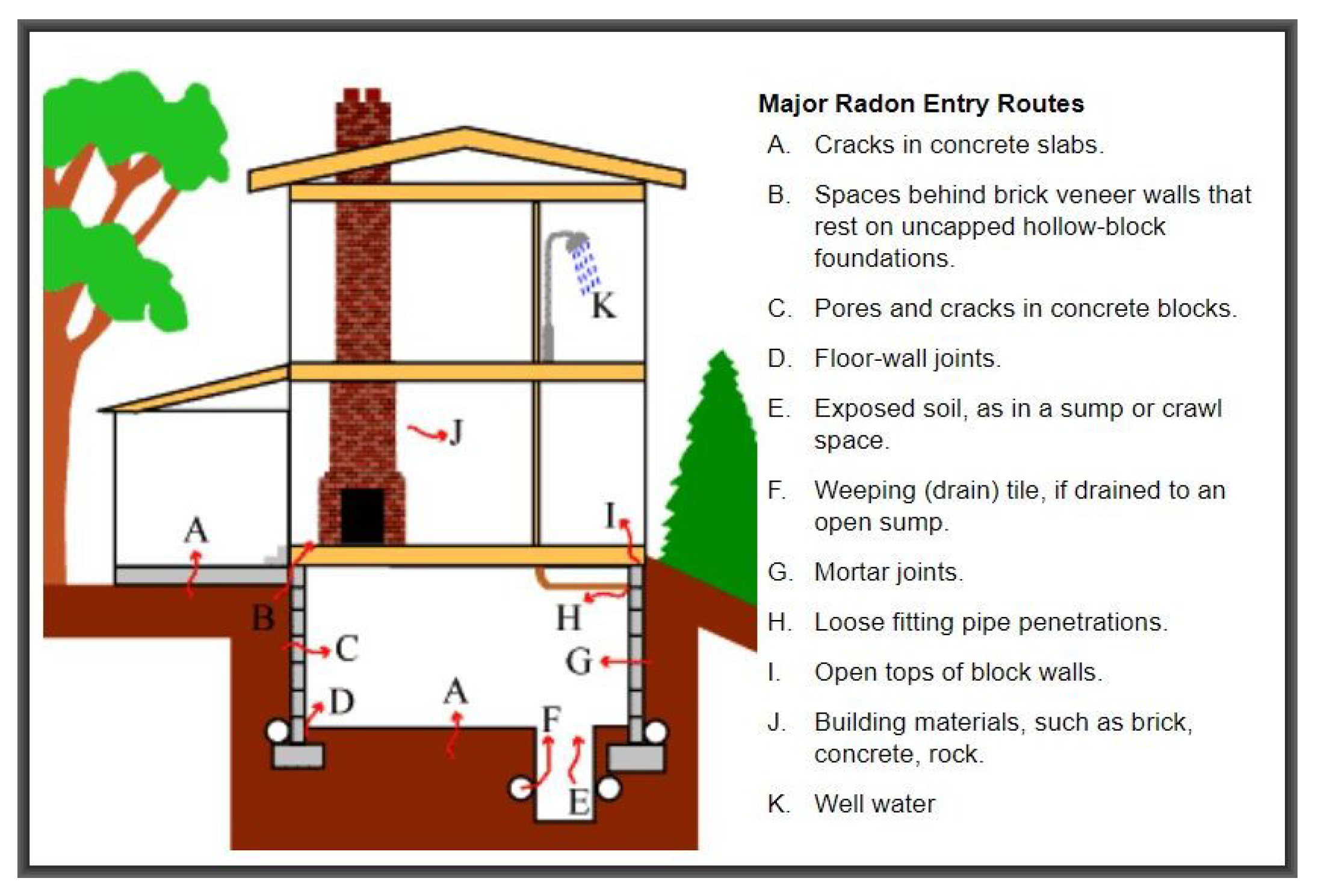
Radon is an inert radioactive gas that occurs naturally in several isotopic forms—the most common being ${}^{222}\mathrm{Rn},$ also referred to as simply radon. Colourless and odourless at ordinary temperatures and potentially soluble in water, the single atom gas easily penetrates many household and workplace materials such as paper, leather, furniture, most paints, concrete, gypsum and other building and insulation material. With a half-life of 3.8 days, radon is formed through the decay of radium-226 in the uranium-238 decay series, forming a number of short-lived radioactive decay products—also known as radon progeny, with much shorter half-lives than radon. The risks of ionising radiation from exposure to radon and its decay products are well-documented [1,2]. While there is little concern over radon released into the open air, as it usually dilutes, there are serious concerns regarding radon released into enclosed places such as homes, office blocks and schools, as the gases can potentially accumulate to high levels and pose serious health risks to the dwellers and frequent users of such premises. As graphically illustrated in Figure 1, there are various ways in which radon gas may enter buildings. Typically, the air pressure inside a building would be lower than it is in the soil surrounding its foundation, which causes air and other gases including radon to be drawn into the building. Any opening with a direct contact with the soil—cracks in foundation, joints, gaps around service pipes, support posts, window casements, floor drains, cavities, etc., would facilitate the flow. Unless there is immediate escape, it soon becomes a health hazard. Exposure to radon in homes and workplaces has for long been known to be linked to lung cancer deaths [3] and so one of the obvious mitigation measures would be to identify emerging patterns of exposure to help guide public health policy. That is, for researchers and relevant authorities to develop methods and tools for uncovering knowledge based on robust scientific evidence to guide public health policies.

Spatial-temporal and other statistical variations of radon have been extensively examined [4,5]. Various data modelling and comparative methods have been applied in many studies, including Ref. [6] who used simple correlation and Principal Component Analysis (PCA) to identify potential relationships among individual local meteorological parameters with a potential impact on ${}^{222}\mathrm{Rn}$ concentrations—i.e., temperature, barometric pressure and relative humidity. Concentration of radon progeny in air depends on, inter-alia, soil properties such as moisture content and porosity [7]. It also depends on meteorological conditions such as rainfall, temperature and pressure as well as wind speed and direction. One part of our radon variations’ analyses, in Section 3, considers these variables.

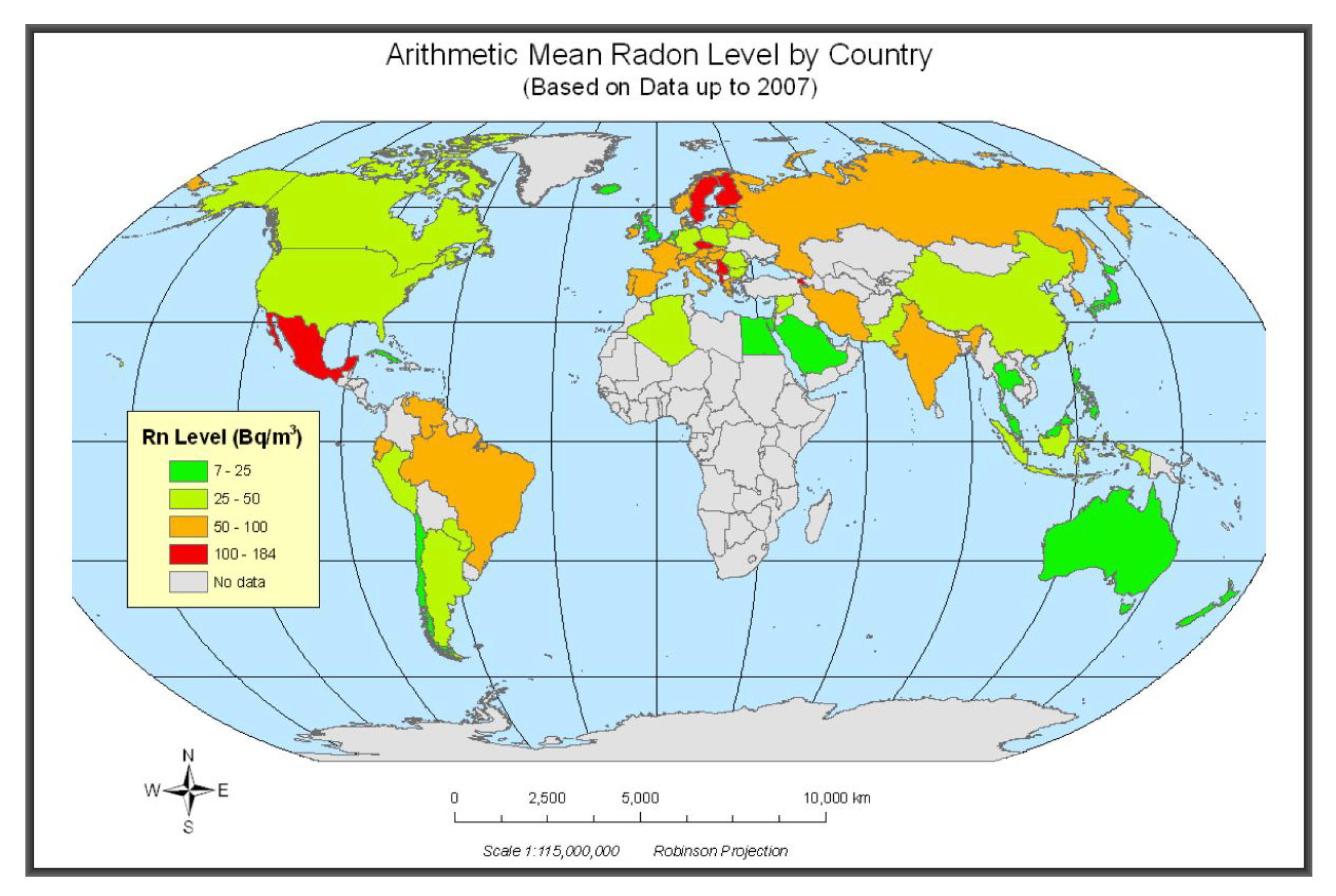
In recent years, harnessing knowledge on the environmental conditions that affect our health, general livelihood and sustainability has attracted great scientific research interest [9,10] and [7]. In this paper, we present a novel approach to modelling radon gas using data collected from passive devices distributed across the city of Doha as well as from a laboratory based real-time radon gas reader. The choice of Doha as a focal study area is motivated by the well-documented lack of radon gas data mapping in parts of the world, including Qatar [11] as shown in Figure 2.

The paper’s main idea derives from the procedure in [6] who compared desert ambient ${}^{222}\mathrm{Rn}$ concentrations from continuous and integrating instruments to characterise and baseline its environmental parameters. Thus, we provide a comparative analysis of the radon variations within the city, aimed at setting the scene for future studies in uncovering linkage between radon exposure and various types of cancer such as those conducted elsewhere [12,13]. We combine exploratory, visualisation and estimation methods to try and answer the question: What is the overall exposure to radon gas of the people in and around Doha? We shall be seeking to extract a general understanding of spatio-temporal variations of the gas via the following objectives:

• to carry out data exploration, visualisation and estimation of radon concentration,
• to analyse technical performances of passive and active radon detectors and their suitability for application,
• to recommend mitigating intervention to policy makers.

The foregoing objectives are partly in line with the general requirements of the International Commission on Radiological Protection (ICRP), the World Health Organization (WHO) and the International Atomic Energy Agency (IAEA)—all of which encourage member states to create in-country programs on radon. More specifically, member states are required to advise the public on radon in homes and workplaces, provide guidelines for locating buildings with radon, check for radon risks prior to starting new construction and introduce limits for concentrations of natural radioactive elements in building materials. Last but not least, variations due to measurement types and standards have been widely reported. Chapter 2 of the World Health Organisation handbook [14] explores radon measurement issues relating to devices, protocols and quality assurance. The paper is organised as follows: study methods, data sources and modelling strategy appear in Section 2, results and discussion are in Section 3, and concluding remarks are in Section 4.

2. Methods

This section provides a general description of our adopted procedure, data sources and modelling strategy. It derives from the procedure in [6] who compared desert ambient ${}^{222}\mathrm{Rn}$ concentrations from continuous and integrating instruments in order to characterize and baseline its environmental parameters. Their work involved deploying passive integrating and continuous radon monitoring instruments for real-time ambient gamma exposure and used meteorological data to correct the readings. Our approach, described in the next sub-sections, uses data collected from passive and active radon detectors to explore, visualise, estimate and interpret radon data concentration patterns in and around the city of Doha—spanning across a period of two years and providing a good coverage of Qatar weather seasons.

2.1. Data Sources

Figure 3 shows the physical data collection spots. A total of 36 passive detectors were deployed in various residential areas, workplaces and schools in and around the city of Doha and its adjacent municipalities. Data also came from an active radon detector located at the Central Radiation Laboratories (CRL) in the Mesaimeer area via the processes described below.

2.1.1. Data From Passive Sources (LLT-OO E-PERM)

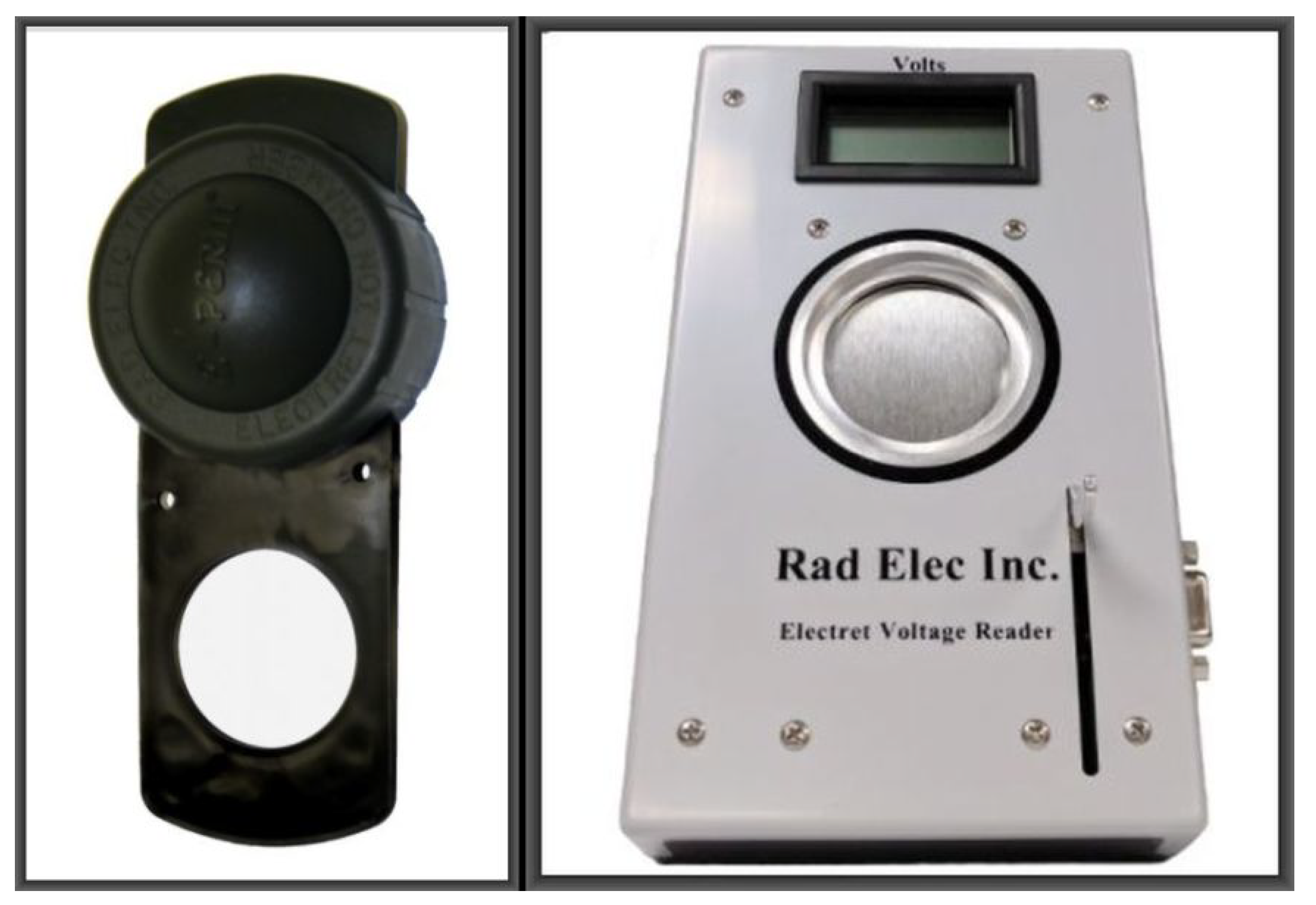
The LLT-OO Chamber radon detector is a passive integrating ionization monitor consisting of a very stable electret mounted inside a small chamber made of electrically conducting plastic. The electret, a charged Teflon disk, serves as both the source for ion collection and as the integrating ion sensor. Radon gas passively diffuses into the chamber through filtered inlets, and alpha particles emitted by the decay process ionize air molecules. Negative ions produced inside the chamber are to be collected on the positively charged electret, causing a reduction of its surface charge. The reduction in charge is a function of the radon concentration, the duration of the testing period, and the chamber volume. A hand-held Rad Electret voltage device with voltage accuracy of $\pm 1$ volt is used to read and provide a measure of the change in voltage. Only two electret voltage readings (initial and final) are read off the device and several steps and conversions are needed to convert these two readings and the exposure period into ${}^{222}\mathrm{Rn}$ concentrations. There is a wide range of parameters affecting radon concentrations—they include detector type, volume of chamber, exposure period, initial-final detector voltage, elevation above sea level and gamma dose rate. The uncertainties of radon concentrations can be be estimated by standard aggregating methods.

With a volume of 58 ml, the L-OO Chamber plus LT (Long Term) electrets work well for longer deployments or in areas with a known high radon concentration [15]. Its slide mechanism allows the chamber to be easily turned on and off to begin and finish radon tests at specifically determined times. Figure 4 shows the device (left-hand side panel) alongside the electret reader (right-hand side panel) [15] that was used to capture and read off data from the Doha neighbourhoods. In

Table 1. Passive data attributes.

Variable	Description
location	Geo-location in or around Doha
position	Polar position of the geo-location
start	Date the device was initially deployed
end	Date the device was finally stopped
days	Total number of days it was deployed
startvolt	Initial volt reading upon deployment
endvolt	Final volt reading
midvolt	Average volt reading
diffvolt	Difference volt $\left(\mathbf{startvolt}-\mathbf{endvolt}\right)$
radonPCiL	Radon–pCi/L (Pico-Curie per liter)
radoncalcula	Radon calculation quantity in Bq/m${}^3$ (Becquerel per cubic metre)
uncertainty	An adjustment quantity (%) for radon calculation
radon	Radon concentration in Becquerel per cubic metre Bq/m${}^3$

, the variables used in our analyses alongside the constants, are mentioned below.

About 200 of these radon detectors were deployed in homes, schools, and workplaces for several months, but for data quality and other reasons, only approximately 75% of these were able to generate useful data, and, after removing data thought to be unreliable, only 36 useful observations remained for the exploratory and visualisation analyses in Section 3. Calculation of the radon concentration is a process that goes through several steps as illustrated below:

$$\mathbf{radonPCiL}=\left[\frac{\mathbf{diffvolt}-0.066667\times \mathbf{days}}{\left[A+B\times \left(\left(\mathbf{startvolt}+\mathbf{endvolt}\right)/2\right)\right]\times \mathrm{days}}-BG\times G\right]\times ECF,$$

(1)

where $A,B$ and G are chamber-specific constants, $\left(\mathbf{startvolt}+\mathbf{endvolt}\right)/2$ is the mid-point voltage, $A+B\times \left((\mathbf{startvolt}+\mathbf{endvolt})/2\right)$ is the calibration factor and $ECF$ is the elevation correction factor—only applicable for elevations above 60 metres for the LLT-OO. A total of 36 observations on 13 variables (Table 1) were used, alongside constants—elevation, Gamma and electret. In order to calculate the final radon concentration, two more quantities are required—radoncalcula, defined as $\mathbf{radonPCiL}\times 37,$ since 1  pCi/L=37 Bq/m${}^3,$ and uncertainty, defined as

$$\mathbf{uncertainty}=\sqrt{{\left[{\alpha }^2+\frac{\beta }{\mathbf{diffvolt}}\right]}^2+{\left[\frac{\gamma }{\mathbf{radoncalcula}}\right]}^2},$$

(2)

where $\alpha ,\beta \mathrm{and}\gamma$ are device-specific parameters. To obtain the final radon concentration—radon—the following conditional test is done. If $\mathbf{uncertainty}\ge 50$OR if $\mathbf{radoncalcula}<-1,$ the lower limit of detection—LLD is recorded, otherwise, $\mathbf{radon}=\mathbf{radonPCiL}.$ We discuss the implications of this method in Section 3 and Section 4.

2.1.2. Data from Active Radon Detector—AGS

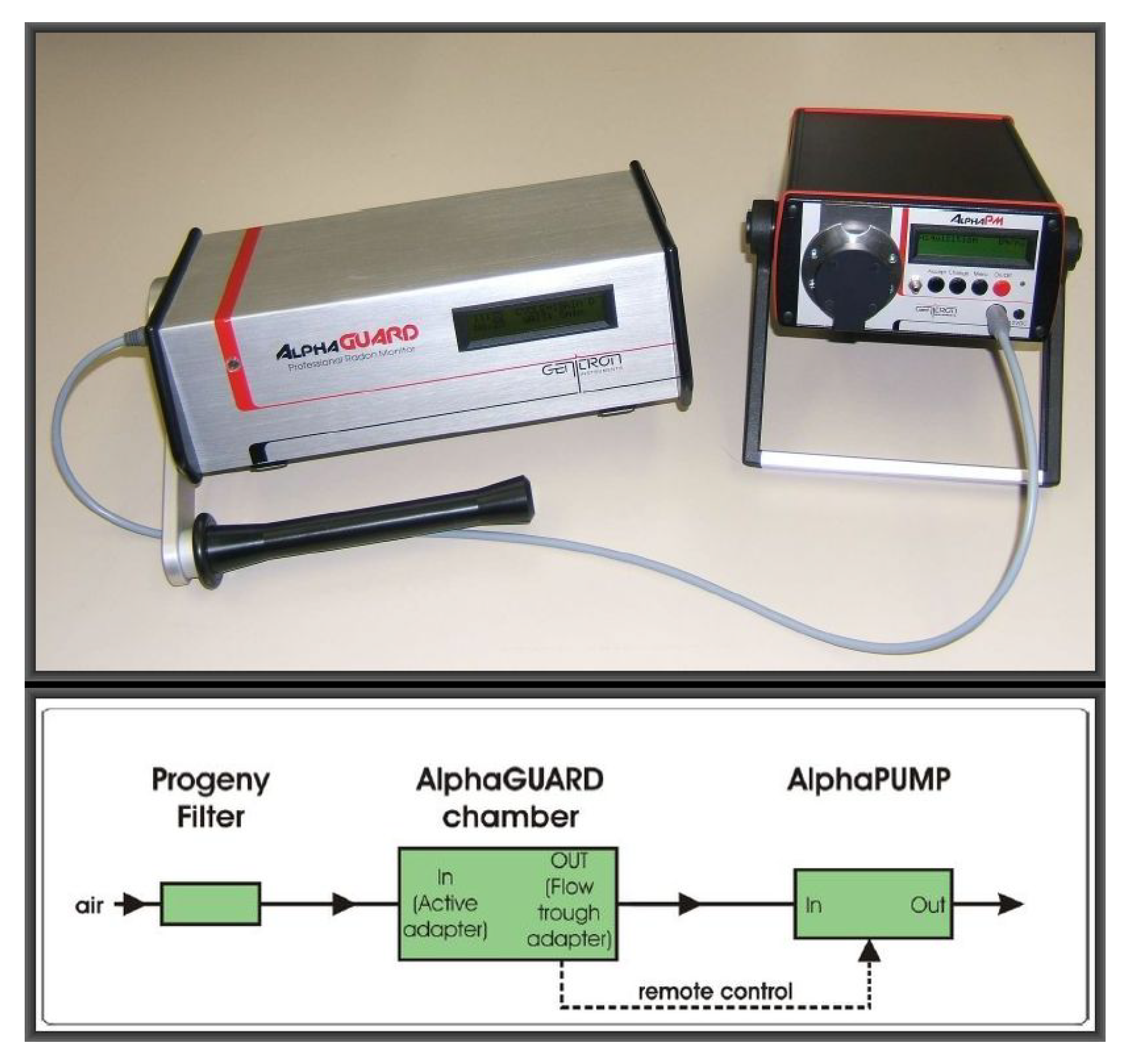
The Alpha Guard System (AGS) utilises pulse-ionization to measure radon and it requires external electrical power or use of the internal battery. Radon diffuses through a fibre-glass filter into a $0.56\mathrm{litre}$ counting chamber. The filter diffusion characteristics are designed to allow for the decay of ${}^{220}\mathrm{Rn}$, (half-life of ∼56 seconds), a progeny of the naturally occurring radioisotope thorium-232. As the Radon, and progeny decay within the chamber, the air is ionized and the ions are attracted to either the cathode or anode producing an electrical pulse, which is processed via a series of internal algorithms generating and recording radon measurements at set frequencies and average concentrations—i.e., every 10 min. Its downside is that it has limited storage capacity and depending on the set frequency data must be downloaded periodically to prevent data loss through data overwrite. Recorded data alongside calculated uncertainties are retrievable by connecting the AGS to a computer running the specialised package DataExpert with an option to generate an Excel file from the data. Unlike the passive devices, the AGS is equipped with environmental sensors designed to monitor air temperature, barometric pressure and relative humidity in its immediate vicinity. A total of 4843 observations on six variables, as summarised in

Table 2. Active data attributes.

Variable	Description
time	Time in hh:mm:ss
radon	Concentrations in Bq/m${}^3$
raderror	Concentration+error in Bq/m${}^3$
pressure	Air Pressure in mbar
humidity	Relative Humidity in %
temperature	Temperature in Celcius
dose	Dose rate in nSv/h

, were generated by the AGS.

Figure 5 [16] shows the AGS in a deployed mode for simultaneous monitoring of radon and its decay products (top panel) while the bottom panel shows the setup and flow direction of gas with the radon/thoron mode. We seek to explore relationships between the variables in Table 2—the behaviour of radon over a long near continuous detection period. The general strategy for attaining the foregoing objectives is outlined below.

2.2. Implementation Strategy

For both objectives 1 and 2 in Section 1, we can use a combination of parametric and non-parametric methods to explore and visualise radon patterns from both detectors. A natural way to do this would be to take an unsupervised approach via which data objects are clustered according to their homogeneity. Data clustering is a standard method in statistical analysis and potentially leads to parameter estimation and likelihood [17,18]. Thus, we can generally let

$$\mathcal{X}=\left\{{\mathbf{v}}_1,{\mathbf{v}}_2,\dots ,{\mathbf{v}}_{p-1},{\mathbf{v}}_p\right\}\subset {\mathbb{R}}^n$$

(3)

and assume k distinct clusters for $\mathcal{X}\mathrm{i}.\mathrm{e}.,\mathcal{C}=\left\{c_1,c_2,\dots ,c_k\right\}$ each with a specified centroid. Then, for each of the vectors $j=1,2,\dots p,$ we can obtain the distance from ${\mathbf{v}}_j\in \mathcal{X}$ to the nearest centroid from the set $\left\{{\mathbf{x}}_1,{\mathbf{x}}_2,\dots {\mathbf{x}}_k\right\}$ as

$${\mathcal{D}}_j\left({\mathbf{x}}_1,{\mathbf{x}}_2,\dots {\mathbf{x}}_k\right)=\underset{1\le l\le k}{min}d\left({\mathbf{x}}_l,{\mathbf{v}}_j\right),$$

(4)

where $d\left(.\right)$ is an adopted measure of distance and the clustering objective would then be to minimise the sum of the distances from each of the data points in $\mathcal{X}$ to the nearest centroid. That is, optimal partitioning of $\mathcal{C}$ requires identifying k vectors ${\mathbf{x}}_1^{\ast },{\mathbf{x}}_2^{\ast },\dots ,{\mathbf{x}}_k^{\ast }\in {\mathbb{R}}^n$ that solve the continuous optimisation function in Equation (5):

$$\underset{\left\{{\mathbf{x}}_1,{\mathbf{x}}_2,\dots ,{\mathbf{x}}_k\right\}\in {\mathbb{R}}^n}{min}f\left({\mathbf{x}}_1,{\mathbf{x}}_2,\dots ,{\mathbf{x}}_k\right)=\sum _{j=1}^p{\mathcal{D}}_j\left({\mathbf{x}}_1,{\mathbf{x}}_2,\dots ,{\mathbf{x}}_k\right).$$

(5)

This minimisation of the distances will depend on the initial values in $\mathcal{C}$ and hence, if we let $z_{i=1,2,\dots ,n}$ be an indicator variable denoting group membership with unknown values, the search for the optimal solution can be through iterative smoothing of the random vector $x\left|\right(z=k),$ for which we can compute $\overline{\mu }=\mathbf{E}\left(x\right)\mathrm{and}\delta =\left\{{\mu }_k-\overline{\mu }|y=k\in {\mathbf{c}}_z\right\}.$ In a supervised scenario—with labelled data, $\left\{x_i,y_i\right\}i=1,2,\dots n,$ Equation (5) amounts to minimising

$$f\left(\theta \right)=\sum _{i=1}^n{\left[y_i-g\left(x_i;\theta \right)\right]}^2,$$

(6)

where $x_i$ are described by $\left\{\overline{\mu }\mathrm{and}\delta \right\}\in \theta .$ Thus, for the data from passive detectors, we shall be looking for features that are reflective of variant or invariant behaviour of these parameters across the deployment locations and periods.

For the active data, we explore various values of the methods’ smoothing parameter to provide different sizes of the neighbourhood to minimise the effect of different types of randomness on the results [19,20]. With Loess—Local Regression, we fit multiple regressions in local neighborhoods of the radon flow from the active detector. We assume the radon concentrations to be bound within the range suggested by the passive devices and the national acceptable limit as shown above. With the passive detectors only providing two readings, this approach is potentially useful for simulating values for the test centres performing least squares regression within localized subsets.

Algorithm 1 provides general mechanics for estimating crucial parameters of radon and related likelihoods. Our interest is in obtaining a set of parameters $\Theta \left\{.\right\}$ that makes the target variable as accurate and as consistent as possible. In practice, this amounts to tracking the variability across and testing, i.e., $\mathbf{Var}\left[\Delta \right]$ as an indicator of stability/variability across models. Note that $C_{y|x.j};j=1,2,3,\dots ,K;i=1,2$ is readily adaptable to the problem at hand—e.g., K-Means for unlabelled data or Random Forest for labelled data and, in both cases, it seeks to minimise over-fitting.

Algorithm 1 Adaptable to Unsupervised and Supervised Modelling

1: procedureGeneral Modelling Mechanics(${\mathcal{C}}_{z|x.j}$) 2:   $\mathbf{Let}{\mathcal{C}}_{z|x.j};j=1,2,3,\dots ,K;i=1,2,\dots r\mathrm{be}\mathrm{classifiers}$ 3:   $\mathbf{Initialise}:\Theta \left\{.\right\}\leftarrow \theta \leftarrow {\mathcal{C}}_{z|x.j}\left\{\mathrm{Initial}\mathrm{Parameters}\right\};\mathrm{Vector}\mathrm{of}\mathrm{Sample}\mathrm{Sizes}\mathbf{s};m:=0,M\left(Large\right)$ 4:   while $m\le M$ do 5:     ${\mathcal{S}}_m\leftarrow m^{\mathrm{th}}\mathrm{sample}{x}_{m.i,j}\subset {\mathcal{X}}_{i,j}$ 6:     $\mathbf{Fit}\mathcal{C}\left(z_m|x_{m.i}\right)\propto \frac{{\pi }_{m.j}{f}_{m.j}\left(x\right)}{{\sum }_{j=1}^k{\pi }_{m.j}{f}_{m.j}\left(x\right)}\leftarrow {\widehat{C}}_{m.z|x_{m.j}\left({\mathcal{S}}_m\right)}$    7:     $\mathbf{Update}m:=m+1$ 8:     $\mathbf{Update}{\Theta }_m\left\{.\right\}\leftarrow {\widehat{C}}_{m.y|x_{m.j}\left({\mathcal{S}}_m\right)}$ 9:     $\mathbf{Update}:{\theta }_m\left\{.\right\}\leftarrow C_{y|x.j}\left\{\mathrm{Fitted}\mathrm{Parameters}\right\};\mathbf{s}:=0$ 10:     $\mathbf{Set}\mathrm{Acceptance}\mathrm{Criteria}{\widehat{C}}_{\mathrm{m}.\mathrm{s}.\mathrm{crit}}\propto {\widehat{C}}_{m.z|x_{m.j}\left({\mathcal{S}}_m\right)}$ 11:     for $\mathbf{s}=1\to \mathrm{Length}\mathrm{of}V$ do 12:       if ${\widehat{\mathcal{C}}}_{m.s.z|x_{m.s.j}\left({\mathcal{S}}_{m.s}\right)}\cong {\widehat{\mathcal{C}}}_{\mathrm{m}.\mathrm{s}.\mathrm{crit}}$ then 13:         $\mathbf{Update}{\Theta }_{m.s}\left\{.\right\}\leftarrow {\theta }_m\left\{.\right\}\leftarrow {\widehat{C}}_{m.s.z|x_{m.s.j}\left({\mathcal{S}}_{m.s}\right)}$ 14:       else 15:         if ${\widehat{\mathcal{C}}}_{m.s.z|x_{m.s.j}\left({\mathcal{S}}_{m.s}\right)}\neg \cong {\widehat{\mathcal{C}}}_{\mathrm{m}.\mathrm{s}.\mathrm{crit}}$ then 16:           $\mathbf{Update}{\Theta }_{m.s}\left\{.\right\}\leftarrow \mathrm{NULL}$    17:         end if   18:       end if   19:     end for 20:     $\mathbf{Update}{\Theta }_m\left\{.\right\}\leftarrow {\Theta }_{m.s}\left\{.\right\}$ 21:   end while 22:   $\mathbf{Output}\mathbf{and}\mathbf{Assess}\mathbf{Performance}\mathbf{Parameters}\mathbf{in}{\Theta }_m\left\{.\right\}$ 23:   $\mathbf{Select}{\Theta }_m\left\{.\right\}\mathrm{that}\mathrm{maximises}{\widehat{\mathcal{C}}}_{m.z|x_{m.j}\left({\mathcal{S}}_m\right)}\propto \frac{{\pi }_{m.j}{f}_{m.j}\left(x\right)}{{\sum }_{j=1}^k{\pi }_{m.j}{f}_{m.j}\left(x\right)}$ 24: end procedure

3. Implementation, Analyses and Discussion

This section presents implementation results based on the strategy outlined in Section 2.2 and, where possible, on the mechanics of Algorithm 1. It focuses on parameter estimation, modelling and visualisation for both detectors.

3.1. Passive Radon Detectors

We present results from 36 passive detectors deployed in 23 different neighbourhoods, focusing on parameter estimation, exploratory data visualisation and simulations for replicating crucial parameters and patterns of radon variations.

Table 3. Descriptive statistics of 36 passive detectors.

Statistic	Days: Deployed	Radon: Concentrations
Minimum	106.00	8.10
First Quartile	145.00	35.70
Median	192.50	60.35
Mean	184.10	64.56
Third Quartile	206.50	80.85
Maximum	252.00	146.60
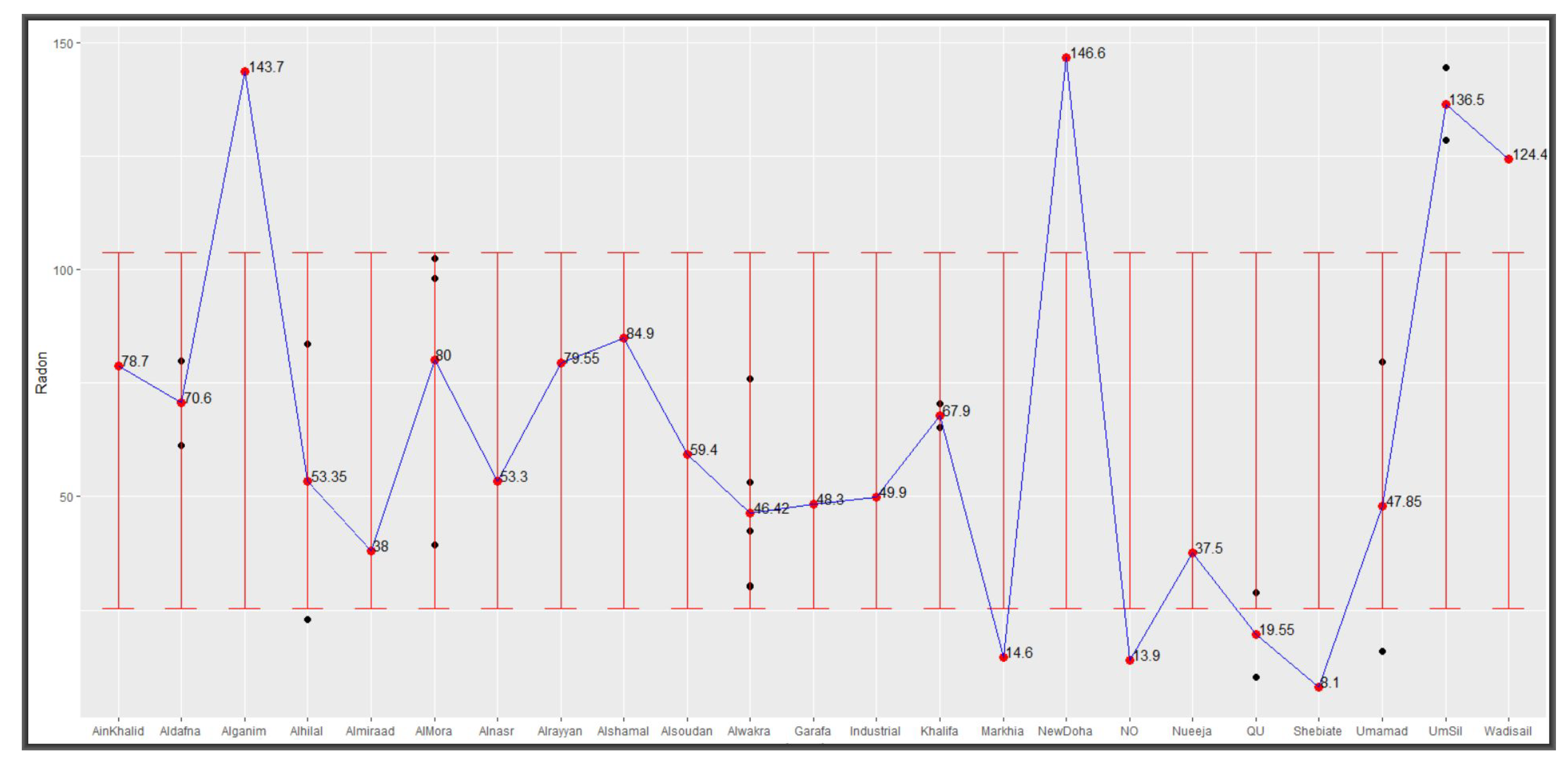
Standard Deviation	43.02	39.25

provides summary statistics for the two variables—number of days and concentrations. With the radon mean at 64.56, the average variation of 39.25 is rather high. Of particular interest was the strong inverse relationship between radon concentrations and uncertainity (61%). While this strong correlation does not necessarily mean we attribute radon concentrations to uncertainty, it highlights the need for further investigations into this detection method. Each device was deployed for at least three months and some remained on site for up to almost nine months. Implicitly, two devices deployed, one for a month and another for six months, are likely to yield approximately readings. Furthermore, the inverse relationship between radon and endvolt suggests that the longer the device remains deployed, the more the readings depend on the initial voltage, suggesting further that there is no benefit of long deployment. It is therefore reasonable to focus on $\left\{\overline{\mu },\delta \right\}\in \theta ,$ particularly on how radon concentrations from various locations vary around these parameters. The black and red dots in Figure 6 show levels of radon concentrations as collected from devices deployed in various locations in and around Doha and their average respectively. Added error bars, based on $\widehat{\mu }=64.56$ and $\delta =39.25291$, show 8 out of the 23 test centres with averages outside the variation interval but all being within Qatar’s acceptable limit of 148 Bq/m${}^3.$ In our final analyses, we explore radon variations around these parameters.

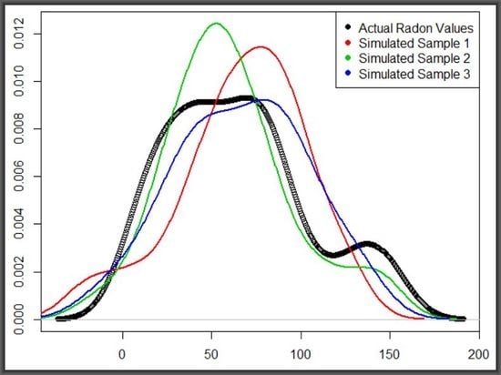
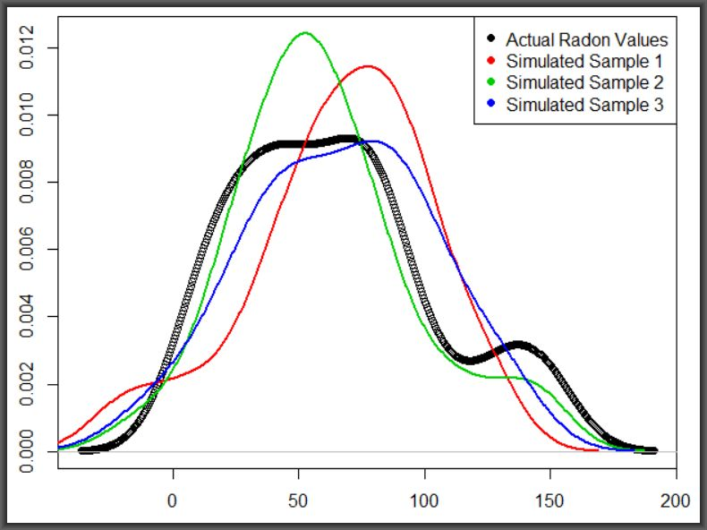
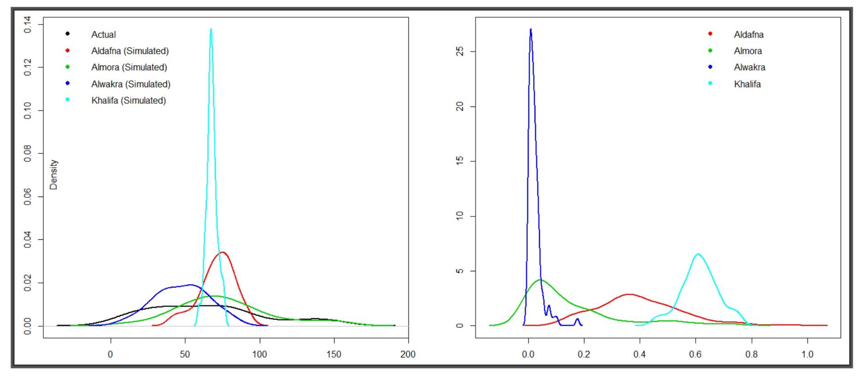
With the exception of Alwakra, which was host to four passive detectors, each of the remaining 35 Doha neighbourhoods had either one or two and with radon concentrations dependent on two parameters, the data sources were constrained. These circumstances provided a motivation for simulating more data to mimick known radon distributions across the neighbourhoods in order to provide a calibrating effect on the detection method. Thus, four neighbourhoods, with meaningful $\widehat{\mu }\mathrm{and}\delta ,$ were selected for data simulation and comparison based on these parameters. The two panels in Figure 7 are results of t-tests for similarity between the overall mean of the 36 locations and that of each of the four test centres. They represent hundreds of simulations of random normal values with mean and standard deviations of the data collected from the centres—i.e., simulated values on the left-hand side and the corresponding p-values on the right. That is, five hundred sample replications were generated and tested for similarity to the overall radon concentration vector. Data from Aldafna and Khalifa exhibited huge departure from the mean, at the 95% level of confidence while only 37% and 10% from Almora and Alwakra, respectively, fell within the acceptable range.

3.2. Active Radon Detectors

This section presents results from the data captured by the Alpha Guard active system—a total of 4843 observations on six variables, as summarised in Table 2. The overall range of radon values generated by Alpha Guard is very different from the range we saw in Section 3.1—a variation that is attributable to the equipment used.

Table 4. Descriptive statistics: Alpha Guard—January 2016 and September 2017.

Time	Statistic	Radon	Radonerror	Pressure	Humidity	Temperature	Dose
January 2016	Minimum	0	3	1011	31.60	19.40	43.00
	1st Quart.	2	3	1014	52	21.10	68
	Median	4	3	1017	60.3	22.50	75
	Mean	4.874	3.713	1017	61.15	22.33	77.27
	3rd Quart.	7	4	1019	71	23.50	84
	Maximum	34	12	1024	85	25.40	156
	STD	4.158	1.158	2.969	12.312	1.486	15.322
September 2017	Minimum	1	3	996	29.50	22.10	49
	1st Quart.	16	7	1000	40.30	24.10	79
	Median	23	9	1002	46.00	24.8	88
	Mean	23.57	9.084	1002	46.84	24.85	88.04
	3rd Quart.	29	11	1004	51	25.4	96
	Maximum	76	22	1008	72	27.60	138.00
	STD	10.25	2.672	2.456	8.548	1.113	12.362

shows summaries of the active readings for the months of January 2016 and September 2017. Used in the analyses below are also radon readings for the months of April, May, June, July and August of 2017. Variable correlations are given in Figure 8 and, as it can be seen, radon does not appear to correlate with any of the meteorological factors. Our final analyses focus on local regression and clustering. In both cases, we aim to determine the optima values for the smoothing parameter and therefore we fit both the loess() function and K-means via Algorithm 1.

Minimising the error—i.e., the smoothing parameter that minimizes the Sum of Squared Errors (SSE) requires lower values of span—which obviously might lead to spurious peaks. Based on different smoothing parameters, we implemented Algorithm 1 to obtain optimal parameters from the predictions by averaging over multiple span runs.

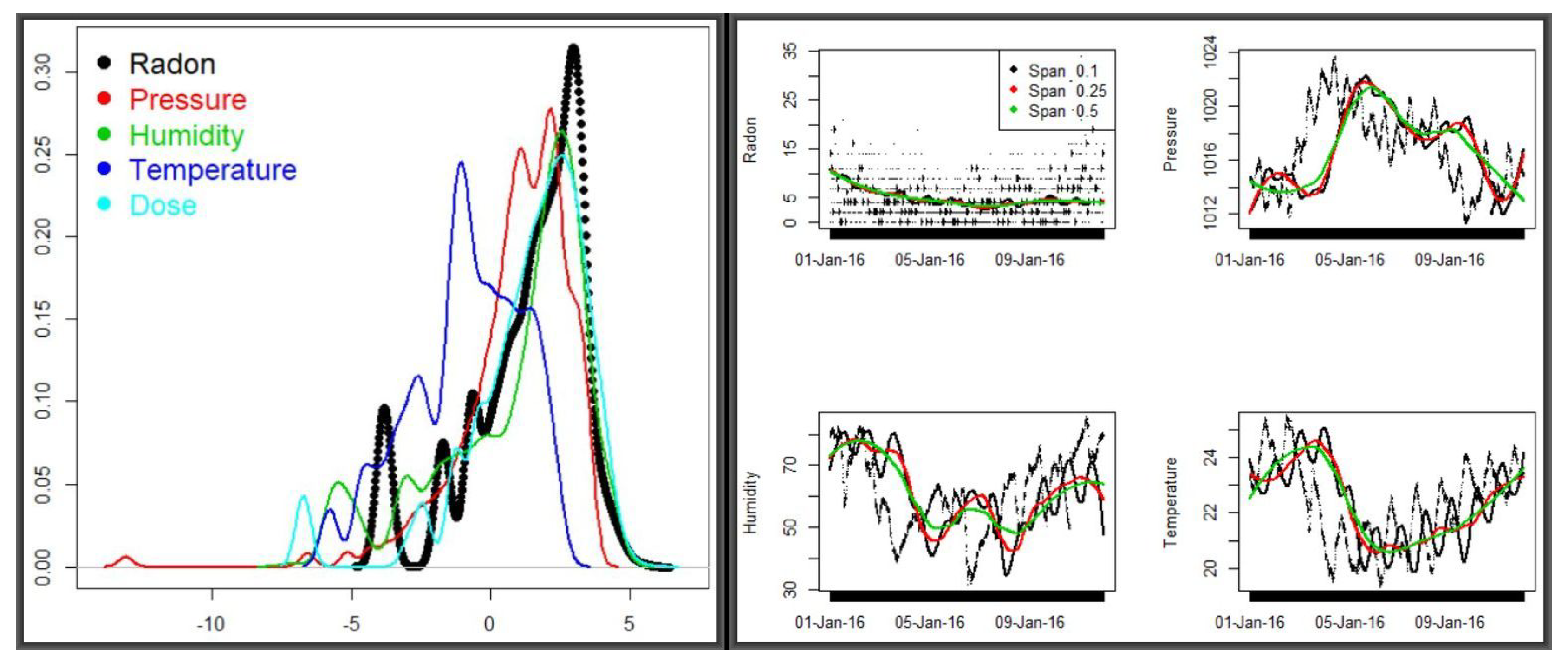
Figure 9 shows the densities for the five variables in the combined dataset (left panel) and the smoothed predictions of radon and meteorologcal variables for two periods of the year (discussed below). Corresponding descriptive summaries for the loess smoothing and predictions of radon and the three meteorological variables—radon, pressure, humidity and temperature are provided in

Table 5. Variable means from loess smoothed predictions for January 2016 and September 2017.

Period	Span	Radon	Pressure	Humidity	Temperature
January 2016	0.10	4.883	1017	61.16	22.33
	0.25	4.870	1017	61.12	22.33
	0.50	4.886	1017	60.88	22.35
September 2017	0.10	23.57	1002	46.83	24.85
	0.25	23.60	1002	46.80	24.87
	0.50	23.49	1002	46.90	24.87

. These variable means were obtained by iteratively refining a span vector of length 40—from 0.025 to 1 at step 0.025. The vector was input to a loess function, updating ${\Theta }_{m.s}$ as in step 13 of Algorithm 1. The three span values yielded the closest estimations to the actual means in Table 4.

The huge variation of radon concentration between the two periods of year was pronounced throughout the spans—but the fact that there are other variables showing little sensitivity to time variations suggests that there must be other factors affecting radon levels. In the next exposition, we carry out two types of analyses—multiple observational and variable clustering, both running through Algorithm 1, for an indication as to which directions to look further. The three panels in Figure 10, left to right, show graphical patterns from the K-Means algorithm on two, three and five centroids, respectively. They are based on radon readings every ten minutes from 30 December 2015 to Sunday, 10 January 2016, combined with those from Tuesday, 29 August 2017 to Thursday, 28 September 2017. The first chunk has 1576 observations with a mean of 4.87 and standard deviation of 4.15, whereas the second consists of 4263 with a mean and standard deviation of 23.57 and 10.25, respectively. All three panels exhibit a huge gap between the first and second chunks of observations, with the former being characterised by low readings and the early readings of the latter starting with extremely high readings and slowly levelling down in mid-September. It may be plausible to attribute the gap to weather variation—also possibly to the data gap between Monday, 11 January 2016 and Monday, 28 August 2017 as the period covers the last days of winter and the onset of summer.

The search for, and optimal testing of, fitted parameters was via Algorithm 1 from which

Table 6. Observational clustering of the radon vector—tested against the samples from the clusters.

Number of Clusters	$\frac{{\mathbf{Between}}_{\mathit{SS}}}{{\mathbf{Total}}_{\mathit{SS}}}\%$	Centroids	Sizes	t-Test vs. $\mathit{\mu }$
$k=2$	66.0%	29.367	2673	0.000000
		9.372	3166	0.000000
		36.715	1177	0.000000
$k=3$	83.5%	5.476	1975	0.162600
		20.148	2687	0.000000
		11.110	940	0.000000
		18.299	1403	0.000000
$k=5$	92.8%	27.483	1546	0.000000
		3.377	1355	0.280000
		41.995	595	0.000000

was generated. The Welch Two Sample t-test was carried out between the full elements of each cluster and a sample of 100 drawn from it in order to determine the representativeness of the centroids with respect to the overall radon readings. The samples were generated as random normal with mean and standard deviation equal to those of the cluster and, despite clear separation between the two chunks of data, sample means hugely differed from those of the two clusters. Table 6 shows that the measure of the goodness of the K-Means classification—i.e., the decomposition of deviance in deviance between and within clusters grows with the number of clusters. Notice that all but two centroids are highly significant. However, the higher the ratio, the higher the cohesion, and we must always be careful as that may lead to over-fitting.

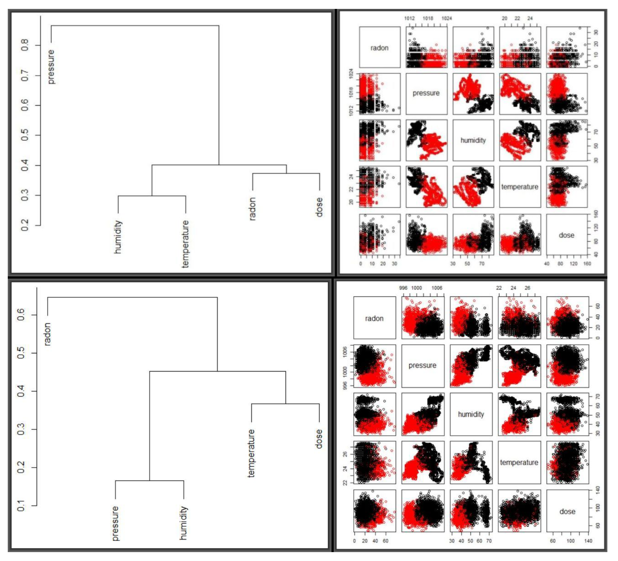
One in the three cluster setting was consistently in agreement with the overall cluster mean, whereas, in the five-cluster setting, this happened only once in 150 runs. It is reasonable to go for three natural clusters in this dataset, but it is imperative to explore factors that may have led to this variation. Figure 11 shows dendograms and and optimal two clusters for the two periods, side by side, scaled by the mean and standard deviation, as shown in

Table 7. Between to Total variation at different scaling and cluster numbers.

Between to Total Variation—at Various Scale and Cluster Numbers
Scaling: January 2016	$\frac{{\mathbf{Between}}_{\mathit{SS}}}{{\mathbf{Total}}_{\mathit{SS}}}\%(\mathit{k}=\mathbf{2})$	$\frac{{\mathbf{Between}}_{\mathit{SS}}}{{\mathbf{Total}}_{\mathit{SS}}}\%(\mathit{k}=\mathbf{3})$	$\frac{{\mathbf{Between}}_{\mathit{SS}}}{{\mathbf{Total}}_{\mathit{SS}}}\%(\mathit{k}=\mathbf{5})$
$\frac{x}{\sqrt{x^2}}+1$	56.70%	66.9%	77.7%
$\frac{x-\mathrm{mean}\left(x\right)}{\mathrm{std}\left(x\right)}+0.1$	39.3%	51.0%	60.1%
$\frac{x}{\mathrm{std}\left(x\right)}+1$	39.3%	51%	60.5%
Scaling: September 2017
$\frac{x}{\sqrt{x^2}}+1$	49.00%	56.10%	72.80%
$\frac{x-\mathrm{mean}\left(x\right)}{\mathrm{std}\left(x\right)}+0.1$	29.50%	37.3%	56.70%
$\frac{x}{\mathrm{std}\left(x\right)}+1$	29.90%	37.20%	56.70%

. The top two panels represent the January 2016 period while the bottom two correspond to September 2017.

For optimisation, the K-means algorithm was repeatedly fitted via Algorithm 1 compared based on scaling methods and cluster numbers and yielding two optimal clusters with clearer separation observed for September 2017 than for January 2016. Columns 2, 3 and 4 of Table 7 were obtained from hundreds of candidate simulations, based on eight scaling methods and cluster numbers between 2 and 15. For both periods, scaling about the mean and standard deviation yielded the best results, with tests similar to those in Table 6 suggesting that three clusters were optimal for both periods. A larger number of clusters yielded very high between to total variation, which, as we explain below, is susceptible to over-fitting. Finally, the mclust [21] also performed better on the data with Algorithm 1 than without.

For both sets of results presented in Table 6 and Table 7, it is worth noting that the algorithm updates cluster centers, allocating observation as it moves until the set condition is met or the change of within-cluster sum of squares in successive iterations becomes insignificant. Updated cluster centers are associated with a measure of the total variance in the dataset that is explained by the clustering. The goal is to minimize the within cluster variation and maximize the between-cluster variation dispersion. However, while we want a higher proportion of between to total variation—as it represents the variance in the data set that is explained by the clustering—i.e., a reduction in sums of squares in percentage, we do not want to overfit the data, as this is what is potentially likely with cluster numbers 5 and above.

4. Conclusions

This paper focused on modelling radon variations in the city of Doha and, despite being specific to that city, many lessons were learned. The study set low level objectives, which we believe were all met as defined but opened new paths for research. This was the first radon study to be conducted in Doha and we expect that our findings will readily be extended to other urban areas where residential workplaces and industrial installations overlap. Although not detailed in this study, such extensions, potentially motivated by geogenic, architectural and general life style conditions, may open new paths towards our understanding of the impact of radon on human health.

4.1. Study Evaluation

Although dependence of the radon level on meteorological factors, nature of building materials, and basement ceilings was not particularly evident in our study, it is usually known to complicate detection mechanisms. A comparative study of short-term (activated carbon) and long-term (alpha particle track) detectors conducted by [22] in a confined geographic area in northwestern Spain yielded a mild correlation between the two detectors, deployed in 391 homes. Overall, readings from short- and long-term detectors didn’t always agree, but high correlations were observed for unventilated homes, coastal sites and the old buildings. As the Spanish Northwest is particularly known for high radon concentrations, these findings can be incorporated in drawing our conclusions—particularly on spatio-temporal radon modelling. The worldwide acceptable recommendation is to measure the radon using passive detectors over a period of one year and this just about what was done in this study. In the aftermath of the study, it is imperative to highlight several challenges. Doha—the subject of this study—is generally characterized by low radon concentrations compared to global levels. The immediate consequence of this is that deployed detectors and calculations of radon concentrations need to be adapted to the local conditions, an issue that has already been raised with the manufacturers of the detectors used in this study. The LLT-OO type of chamber is probably not the best choice for low radon concentration countries and future studies may have to use a combination of large volume chambers and more sensitive detectors. Its suitability for 4- to 12-month deployment assumes that radon concentrations are constant throughout the period and hence it takes the average of the two readings as the location’s representative. Thus, we would like to consider this study as a pilot—constrained by both detectors and area coverage. A national plan requires thousands of detectors covering the residential areas, schools, and work places—the success of which depends much on inter-ministerial decisions—more specifically, on resources allocation and approval by the ministries of interior and municipality and environment. The active detector was located in a single laboratory in the Mesaimeer area of Doha, which may be highlighted as a weakness of the study. However, under the circumstances, it was the only practical tool available that was capable of providing insights into radon and other meteorological factors over months, days and minutes. Furthermore, Doha’s underlying geological formation is almost the same across the city and neighbourhoods, which suggests that the exhale rate of radon from the soil is almost equal across neighbourhoods.

4.2. Future Directions

Environmental factors tend to affect groups of people that share common habitats—residential and working. Identifying and understanding their role as human health predictors potentially helps explain spatio-temporal variations and patterns and mitigation. Thus, while the approach was applied to a geographically confined Doha neighbourhood and over a short period of time, similar analyses and comparisons can be made across continents, countries and wider regions over longer periods of time. Thus, it would be interesting for future studies to map radon variations on specific health conditions within Doha neighbourhoods and beyond. They may, particularly, focus on capturing systematic interactions among a broader category of pollutants such as hydrocarbon, air particulate carbon monoxide and nitrogen dioxide; and monitor radon variations against carbon monoxide at specific time periods of the year or air particulate versus radon levels at different humidity levels. Most importantly, such studies may map pollutants to health conditions, such as lung cancer across various parts of the country. Such extensions are particularly appealing because health risks from radon exposure have been a priority among the top global health institutions as stated in Section 1 and, as reported in [23], while differentiating factors of spatial-temporal variations may be more pronounced across countries, there is sufficient evidence that noticeable differences across regions and neighborhoods within cities exist. This study has the potential to provide lessons for and learn from other countries—particularly those well-documented radon patterns. For instance, both [24,25] studies were carried out in two of the 34 countries listed by [11] as having thorough radon data mappings and they both highlight how radon exposure can be reduced through mitigation measures. Thus, given the measurement variations uncovered in our study, it is extremely important that research findings are widely shared—that is, ensuring that data, findings and modelling approaches are archived and shared among researchers and that there is continuity to such studies. For that purpose, the data, tools, and methods used in this study will be kept available in the project’s archives and it is our expectation that this study will have opened new paths for research.

References

- Darby, S.; Hill, D.; Auvinen, A.; Barros-Dios, J.M.; Baysson, H.; Bochicchio, F.; Deo, H.; Falk, R.; Forastiere, F.; Hakama, M.; et al. Radon in homes and risk of lung cancer: Collaborative analysis of individual data from 13 European case-control studies. BMJ 2005, 330, 223. [Google Scholar] [CrossRef] [PubMed]
- Kant, K.; Chauhan, R.P.; Sharma, G.S.; Chakarvarti, S.K. Hormesis in humans exposed to low-level ionising radiation. Int. J. Low Radiat. 2003, 1, 76–87. [Google Scholar] [CrossRef]
- Alavanja, M.C.; Lubin, J.H.; Mahaffey, J.A.; Brownson, R.C. Residential radon exposure and risk of lung cancer in Missouri. Am. J. Public Health 1999, 89, 1042–1048. [Google Scholar] [CrossRef] [PubMed]
- Steck, D.J. Spatial and temporal indoor radon variations. Health Phys. 1992, 62, 351–355. [Google Scholar] [CrossRef] [PubMed]
- Lubin, J.H.; Boice, J.D., Jr.; Samet, J.M. Errors in exposure assessment, statistical power and the interpretation of residential radon studies. Radiat. Res. 1995, 144, 329–341. [Google Scholar] [CrossRef] [PubMed]
- Shafer, D.S.; McGraw, D.; Karr, L.H.; McCurdy, G.; Kluesner, T.L.; Gray, K.J.; Tappen, J. Comparison of Ambient Radon Concentrations in Air in the Northern Mojave Desert from Continuous and Integrating Instruments; Research Institute (DRI), Nevada System of Higher Education: Reno, NV, USA, 2010. [Google Scholar]
- Pinault, J.-L.; Baubron, J.-C. Signal processing of soil gas radon, atmospheric pressure, moisture, and soil temperature data: A new approach for radon concentration modeling. J. Geophys. Res. 1996, 101, 3157–3171. [Google Scholar] [CrossRef]
- EMSL Analytics Inc. Radon Testing Laboratories; EMSL Analytics Inc.: New York, NY, USA, 2011; Available online: http://www.radontestinglab.com/enterhome.asp (accessed on 16 June 2018).
- Song, M.L.; Fisher, R.; Wang, J.L.; Cui, L.B. Environmental performance evaluation with big data: Theories and methods. Ann. Oper. Res. 2016, 1–14. [Google Scholar] [CrossRef]
- Zheng, Y.; Liu, F.; Hsieh, H.P. U-air: When urban air quality inference meets big data. In Proceedings of the 19th International Conference on Knowledge Discovery and Data Mining, Chicago, IL, USA, 11–14 August 2013. [Google Scholar]
- Zielinski, J.M.; Chambers, D.B. Mapping of residential radon in the world. In Proceedings of the 12th International Congress of the International Radiation Protection Association, Buenos Aires, Argentinien, 19–24 October 2014. [Google Scholar]
- Catelinois, O.; Rogel, A.; Laurier, D.; Billon, S.; Hemon, D.; Verger, P.; Tirmarche, M. Lung cancer attributable to indoor radon exposure in France: Impact of the risk models and uncertainty analysis. Environ. Health Perspect. 2006, 114, 1361–1366. [Google Scholar] [CrossRef] [PubMed]
- Krewski, D.; Lubin, J.H.; Zielinski, J.M.; Alavanja, M.; Catalan, V.S.; William Field, R.; Klotz, J.B.; Létourneau, E.G.; Lynch, C.F.; Lyon, J.L.; et al. A combined analysis of north american case-control studies of residential radon and lung cancer. J. Toxicol. Environ. Health Part A 2006, 69, 533–597. [Google Scholar] [CrossRef] [PubMed]
- Zeeb, H.; Shannon, F. Who Handbook on Indoor Radon: A Public Health Perspective; Taylor & Francis: London, UK, 2009. [Google Scholar]
- Rad Elec Inc. Radon Measurement Systems; Rad Elec Inc.: Frederick, MD, USA, 2018. [Google Scholar]
- Saphymo GmbH. AlphaGuard Portable Radon Monitor; Saphymo GmbH: Berlin, Germany, 2018. [Google Scholar]
- Chapmann, J. Machine Learning Algorithms; CreateSpace: North Charleston, SC, USA, 2017. [Google Scholar]
- Kogan, J. Introduction to Clustering Large and High-Dimensional Data; Cambridge University Press: Cambridge, UK, 2007. [Google Scholar]
- Mwitondi, K.; Moustafa, R.; Hadi, A. A data-driven method for selecting optimal models based on graphical visualisation of differences in sequentially fitted roc model parameters. Data Sci. 2013, 12, 247–253. [Google Scholar] [CrossRef]
- Mwitondi, K.; Said, R. A data-based method for harmonising heterogeneous data modelling techniques across data mining applications. Stat. Appl. Probab. 2013, 2, 293–305. [Google Scholar] [CrossRef]
- Fraley, C.; Raftery, A.E.; Murphy, T.B.; Scrucca, L. Mclust Version 4 for R: Normal Mixture Modeling for Model-Based Clustering, Classification, and Density Estimation; Springer: Berlin, Germany, 2012. [Google Scholar]
- Ruano-Ravina, A.; Castro-Bernárdez, M.; Sande-Meijide, M.; Vargas, A.; Barros-Dios, J. M Short- versus long-term radon detectors: A comparative study in galicia, NW Spain. J. Environ. Radioact. 2008, 99, 1121–1126. [Google Scholar] [CrossRef] [PubMed]
- Roux, D.; Mair, C. Neighborhoods and health. Ann. N. Y. Acad. Sci. 2010, 186, 125–145. [Google Scholar] [CrossRef] [PubMed]
- Petrescu, D.C.; Petrescu-Mag, R.M. Setting the scene for a healthier indoor living environment: Citizens’ knowledge, awareness, and habits related to residential radon exposure in romania. Sustainability 2017, 9, 2081. [Google Scholar] [CrossRef]
- Fuoco, F.C.; Stabile, L.; Buonanno, G.; Trassiera, C.V.; Massimo, A.; Russi, A.; Mazaheri, M.; Morawska, L.; Andrade, A. Indoor air quality in naturally ventilated italian classrooms. Atmosphere 2015, 6, 1652–1675. [Google Scholar] [CrossRef] [Green Version]
Figure 1.
Different ways radon gas can enter a home [8].
Figure 2.
Available global radon mappings by country as of 2014 (Source: [11]).
Figure 3.
The passive devices—mainly deployed in the Doha neighbourhoods with only one in the north.
Figure 4.
The LLT-OO Chamber passive radon detector (L), and the Rad Electret reader (R).
Figure 5.
Physical deployment of the AGS (top) panel and its setup and gas flow direction (bottom) (Source: Bertin Instruments, Montigny-le-Bretonneux, France, https://www.bertin-instruments.com/) [8].
Figure 6.
Radon concentrations and associated averages as gathered from 36 passive detectors.
Figure 7.
Real radon concentrations versus multiple simulations based on and for each of the neighbourhoods (LHS) and the corresponding p-values on the right.
Figure 8.
Top-left clockwise: variable correlations for January 2016 and February, June, and September 2017.
Figure 9.
Densities for the five variables in the combined dataset (LHS) and the standardised smoothed predictions of radon and meteorologcal variables for two periods of the year (RHS).
Figure 10.
From left to right—radon vector clustering results for two, three and five clusters, respectively.
Figure 11.
Dendograms and optimal clusters for January 2016 (top) panels and September 2017 (bottom) panels.