Reynolds Stresses and Hemolysis in Turbulent Flow Examined by Threshold Analysis

Abstract

Use of laminar flow-derived power law models to predict hemolysis with turbulence remains problematical. Flows in a Couette viscometer and a capillary tube have been simulated to investigate various combinations of Reynolds and/or viscous stresses power law models for hemolysis prediction. A finite volume-based computational method provided Reynolds and viscous stresses so that the effects of area-averaged and time-averaged Reynolds stresses, as well as total, viscous, and wall shear on hemolysis prediction could be assessed. The flow computations were conducted by using Reynolds-Averaged Navier-Stokes models of turbulence (k-ε and k-ω SST) to simulate four different experimental conditions in a capillary tube and seven experimental conditions in a Couette viscometer taken from the literature. Power law models were compared by calculating standard errors between measured hemolysis values and those derived from power law models with data from the simulations. In addition, suitability of Reynolds and viscous stresses was studied by threshold analysis. Results showed there was no evidence of a threshold value for hemolysis in terms of Reynolds and viscous stresses. Therefore, Reynolds and viscous stresses are not good predictors of hemolysis. Of power law models, the Zhang power law model (Artificial Organs, 2011, 35, 1180–1186) gives the lowest error overall for the hemolysis index and Reynolds stress (0.05570), while Giersiepen’s model (The International journal of Artificial Organs, 1990, 13, 300–306) yields the highest (6.6658), and intermediate errors are found through use of Heuser’s (Biorheology, 1980, 17, 17–24) model (0.3861) and Fraser’s (Journal of Biomechanical Engineering, 2012, 134, 081002) model (0.3947).

1. Introduction

Artificial hearts and ventricular assist devices create non-physiological blood flow conditions [1], such as turbulence [2,3], causing red blood cell (RBC) damage, an important consideration in the design of prosthetic heart devices. Turbulent flow means that irregular, random, chaotic, and multiscale flow conditions prevail with a wide range of time and length scales that cause harmful effects in blood, because of significant fluctuations in shear stresses and pressure. It is commonly accepted that turbulence effects are important to RBC damage causing hemolysis, i.e., release of hemoglobin from erythrocytes, which increases when cells are exposed to turbulent stresses [4]. While stress levels are well characterized for laminar flow fields, the effects of turbulence structure on hemolysis of blood cells are unclear [4,5,6]. Predicting and understanding the effect of turbulent stresses on erythrocytes would lead to more rational design of prosthetic heart devices [4,5,6].

The factors that are commonly accepted as important to blood damage are the stresses that the cells undergo and the time duration over which the cells are exposed to these stresses. It is unlikely that stress alone can rupture the cell membrane; however, it can cause enough damage to the cell that it can start leaking hemoglobin into the blood stream [7]. The most typical empirical model that includes both stresses and time of exposure is the power law model that can be written in its most general form as follows [8]:

$$HI=C{\mathsf{\tau }}^{\mathsf{\alpha }}{t}^{\mathsf{\beta }}$$

(1)

where HI, hemolysis index, is a measure of hemolysis, τ is shear stress, t is time of exposure to stress τ, and α, β, and C are constants that are experimentally obtained.

Since the values of the parameters appearing in Equation (1) have been obtained through experiments for laminar flow [9,10,11], the applicability of the power law models to turbulent flows is questionable. The main reason is that turbulent flows in medical devices are not isotropic, and the stresses that the cells experience depend on the cell motion as they move through the flow field. The local flow environment, including the presence of flow eddies and pressure and stress local fluctuations can be crucial for damaging the RBC membrane. Such issues generate questions about the accuracy of models based on power law expressions. Similar issues, where laminar models do not work well for turbulent flow situations, are also observed when models for platelet activation are adopted [12,13,14].

Hemolysis has been examined using different stresses (Reynolds, viscous, wall shear, etc.) by several researchers. Which characterization of turbulent stress relates best to hemolysis is an important consideration for application of the power law. If the dependence on Reynolds stresses is similar to what is seen for stresses in laminar flow, then one expects to see a large increase in hemolysis at some threshold value of the Reynolds stress, because of the exponential feature of the power law relationship. However, it has been seen that a value of the threshold turbulent stresses for hemolysis remains unsettled [15]. As such, the main goal of this research is to investigate the effect of time-averaged and area-averaged Reynolds stresses and viscous stresses on hemolysis by conducting a threshold analysis.

In this study, a systematic analysis using computational fluid dynamics (CFD) for two completely different systems has been carried out using a wide range of hemolysis experiments in Couette flow [16] and capillary tube flow geometries [4]. CFD has been widely used to determine hemolysis as a function of flow field conditions found in cardiovascular devices and has often been used to analyze, improve, and optimize Ventricular Assist Devices (VADs) [17,18,19,20,21,22]. Correct measurements of flow parameters, such as the instantaneous spatial distribution of the rate of dissipation of turbulent kinetic energy (ε), are difficult in the laboratory, which makes CFD essential for these systems. The experiments simulated here were performed by different laboratories and include high quality hemolysis measurements. Moreover, these systems have distinctly different flows and exposure times representing a range of experimental conditions yielding data on hemolysis levels. The computational results provide the spatial stress variation for the simulated experiments enabling a useful evaluation of the importance of Reynolds and viscous stresses for hemolysis. In particular, the suitability of various stresses in power law models to estimate hemolysis was examined with the stresses obtained from computations.

This study also considers a different aspect of the power law approach by testing applicability of area-averaged and time-averaged Reynolds, as well as total, viscous, and wall shear stresses using reported power law parameters [10,11,18,23] for the experiments in the capillary tube. The standard error [24] between experimentally measured hemolysis data and theoretical calculations for each stress option was also found. Background information is given in Section 2 and the device geometries used for our analysis as well as the computational techniques are introduced in Section 3. In Section 4, we show results for the Reynolds stress distributions in Couette viscometer and capillary tube experiments. We observe that in each set of capillary flows and Couette viscometer flows, there exists no single consistent Reynolds and viscous stress value above which hemolysis occurs. Therefore, neither Reynolds stress nor viscous stress is a good predictor of hemolysis. We have recently described a relationship between dissipative eddies comparable or smaller in size to RBCs and hemolysis. Such findings may lead to the development of other approaches to predict mechanical trauma with turbulence [25].

2. Background

The power law equation (Equation (1)) was adopted by Giersiepen et al. [23], based on in vitro laminar flow experiments with human RBC, to predict hemolysis downstream of aortic valves. Constants α, β, and C were determined from regression analysis applied to experimental data for shear stresses less than 255 Pa and exposure times less than 700 ms. Heuser and Opitz [10] obtained their set of coefficients using laminar flow in a Couette viscometer to determine hemolysis of porcine blood for exposure times less than 700 ms and shear stresses less than 255 Pa. Zhang et al. [11] examined hemolysis of ovine blood for exposure times of less than 1500 ms and shear stresses between 50–320 Pa and obtained power law constants by fitting the hemolysis results to Equation (1). It has, however, been argued that since power law models were obtained by using viscometer experiments with steady, uniform laminar flow shear stress, the models often fail when capturing the general flow features of typical medical devices [26] which usually impose multiple, shorter term exposures.

Quinlan and Dooley [27] have presented an analysis for both laminar and turbulent flow. In their turbulent flow analysis, a model to predict shear stress on red blood cells was developed by considering the effect of turbulent flow on an isolated cell. They applied their model to prosthetic valve data by Liu et al. [28] and investigated the relationship between true stress on blood cells and the measurable macroscopic stresses. Reynolds stresses are not small enough to directly capture the microscopic flow field in which hemolysis happens [27,29,30,31]. Moreover, the stress distribution on the surface of the cell was affected by complicated local plasma flow around each cell. Quinlan and Dooley suggested that cells are exposed to low stress and acceleration by larger eddies. However, smaller eddies are responsible for causing the cells to experience high velocity gradients and fast velocity changes. Therefore, effect of different length scales on cells cannot be captured separately by using Reynolds stresses [27]. Viscous stresses also characterize blood in macroscopic levels and they are not adequate to resolve the flow field near the cells to determine hemolysis [27]. Lee et al. [32] investigated viscous and Reynolds stresses for three different heart valves. The calculated maximum value of viscous shear stresses was small. Therefore, the effect of viscous stresses on cell trauma was neglected.

The value of Reynolds stresses in predicting blood damage was also investigated by Jones [33]. Local viscous stresses were determined in turbulent flow and it was suggested that using local viscous stresses instead of Reynolds stresses to determine hemolysis was more reasonable [33]. Even though Reynolds stresses were used to correlate hemolysis results in the work of Sallam and Hwang [34], viscous shearing was recommended as a potential mechanism [35,36]. Other researchers have considered Reynolds stresses as having a similar effect as the viscous stresses in laminar flows [28,34,37,38].

In the work of Hund et al. [3], the Navier-Stokes and Reynolds-Averaged Navier-Stokes (RANS) equations were used to mathematically calculate the errors of predicted blood damage. It was found that significant error can be anticipated when Reynolds stresses are used in a power law equation to predict hemolysis. As such, if Reynolds stresses are used in blood damage calculation, the accuracy of predictions would be doubtful [3]. However, Hund et al. also noted surprising success of some groups in predicting hemolysis by using Reynolds stresses. In this study, we examine four different power law models with Reynolds and other stresses for prediction of hemolysis with turbulence.

3. Methods

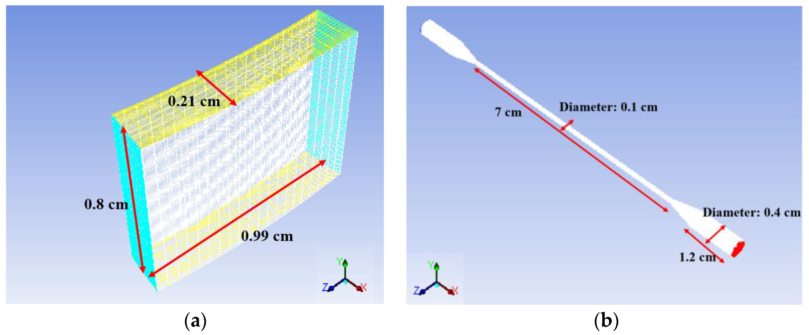
3.1. Modeled Systems

Two different experimental systems with reported levels of hemolysis with turbulence were chosen and simulated using CFD. The simulations were performed for hemolysis experiments in a Couette viscometer and a capillary tube, which offer distinctly different flows with exposure times varied by orders of magnitude.

The first modeled geometry is a Couette viscometer, in which the magnitude of the average shear stress is determined by the gap width and relative rotational speed of the two concentric cylinders. Couette viscometers have been commonly used to study hemolysis [10,39,40], because high shear stresses can be obtained for well-defined laminar flow with relatively short loading times [10]. Couette viscometers have also been used for turbulent flows such as in the work of Sutera and Mehrjardi [16]. In their study, the rotor of the viscometer [16] was 5 cm long, 10 cm in diameter with a rotating inner cylinder and a stationary outer cylinder. A maximum shear stress of 450 Pa was reached by the use of 2.07 mm gap width between cylinders. Hemolysis was determined for a period of 4 min by using washed, human erythrocytes in phosphate buffered saline (PBS)/glucose at low hematocrit (2%). The flow is turbulent in this range of parameters, as is discussed in the next section of this work. To simulate their experiment, 1/32nd of the whole viscometer was modeled (Figure 1a). The size of the section modeled was determined by taking into account the turbulence integral length scales in the computational domain when expressed in dimensionless viscous wall units. (Dimensionless wall parameters are based on the friction velocity, u*, and the viscous length scale, l*, and are typically used in scaling wall turbulent flow. The friction velocity is a function of the fluid density, $\mathsf{\rho }$, and the wall shear stress, τ_w, defined as $u^{*}=\sqrt{\frac{{\mathsf{\tau }}_w}{\mathsf{\rho }}}$, while the viscous length scale is defined from the fluid kinematic viscosity, ν and the friction velocity as $l^{*}=\frac{v}{u^{*}}$). The typical value of the integral length scales in wall turbulence is about 1000 in viscous wall units. The range of the size of our computational domain in the azimuthal direction was changing from 2174 (for the lowest shear stress experiment, 50 Pa) to 6498 (for the highest shear stress experiment, 450 Pa) in viscous wall units. Both values are more than twice the typical value of 1000, justifying the use of 1/32nd of the viscometer in the azimuthal direction for the simulations.

A capillary tube is the second geometry examined, one frequently used to study hemolysis in biomedical practice. Capillary tubes give an opportunity to simply observe hemolysis when changing different parameters such as pipe diameter, length and type of wall surface [41]. The specific system simulated in this study is the capillary tube used by Kameneva et al. [4]. The length and the diameter of the tube are 70 mm and 1 mm respectively and the tube has conically shaped connectors (8 mm length) at each end of the capillary (Figure 1b). Hemolysis experiments were performed by circulating washed bovine red cells in phosphate buffered saline (PBS) at a 24% hematocrit through the capillary in a closed loop network providing multiple short-term exposures to turbulent flow. While the human blood has hematocrit in the range of 40%–55%, the experiments and the results obtained can be used to relate stresses to cell behavior. Capillary tube was in a closed circulating loop which includes a pump, polyvinyl chloride (PVC) tubing, a water bath, a collapsible reservoir, and small glass capillary tube [4]. Time for one circulation of blood in the experimental loop was calculated from volume of blood sample and volumetric flow rates which were specified in the original work [4]. Moreover, the time for one pass of blood through the capillary tube was calculated from the known volume of the capillary tube and experimental volumetric flow rates. The average number of trips around the experimental flow loop was also calculated from a given experimental time and the time for one pass of blood around the loop. Finally, estimated cumulative exposure time of blood was calculated from the total time of the experiment and the time to circumnavigate the loop. Estimated cumulative exposure time was to the order of 1 s. Times for one pass of blood around the loop and number of circulations were different for each experiment. However, cumulative exposure time of blood in each experiment was found to be equal as also stated in the original work [4]. Furthermore, the surfaces of the viscometer and the capillary tube are considered to be neither rough nor biochemically interacting with the cells.

3.2. Computational Procedures

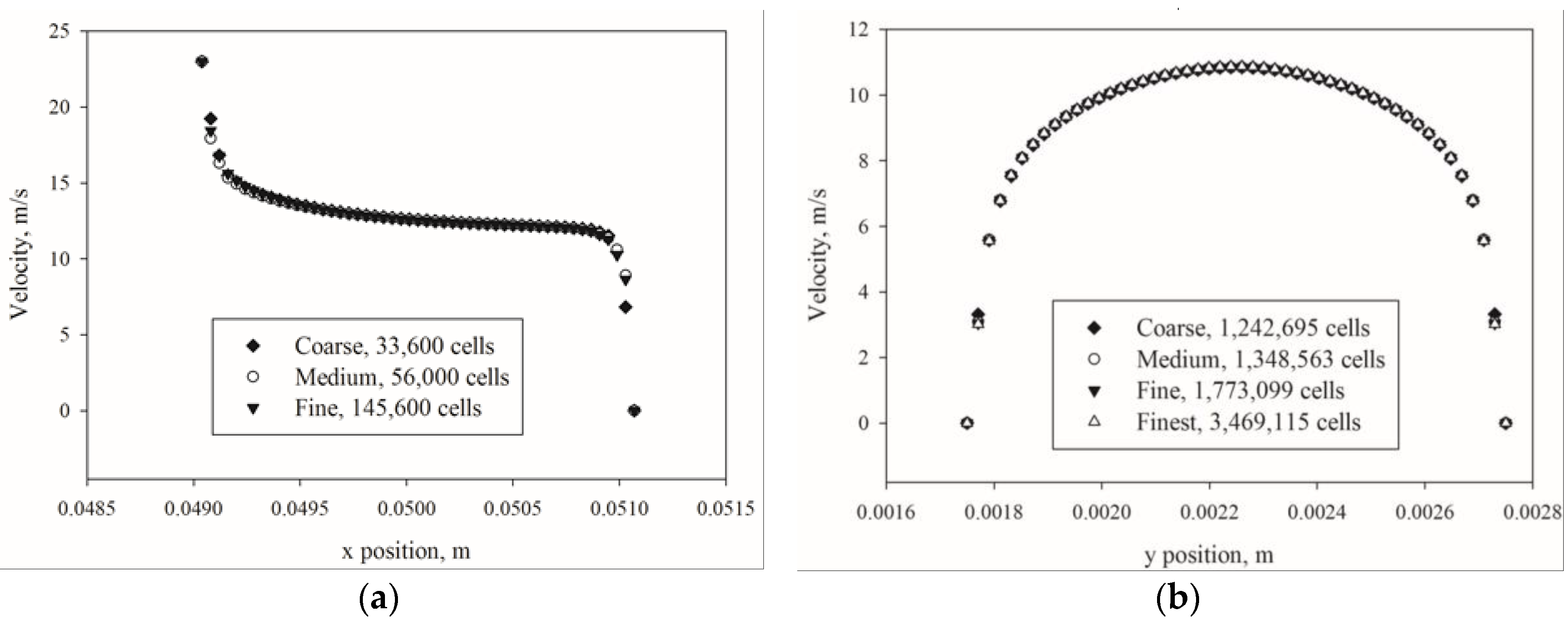
3.2.1. Computational Mesh

The Couette viscometer (Figure 1a) and the capillary tube (Figure 1b) were meshed using Fluent 14.0 and its preprocessing program ICEM CFD (Ansys, Pittsburgh, PA, USA). In the capillary tube geometry, a three-dimensional model of the whole geometry with the conic entrance and exit regions was recreated. Meshing the entire geometries with hexahedral elements was performed after the geometries were created. Moreover, element orthogonality and the mesh quality of the capillary tube was increased by using o-grids around the inlet and outlet region. After mesh creation in ICEM CFD, the flow geometries were imported into Fluent to solve the incompressible Navier-Stokes equations. Mesh independence of the models was tested by refining the grid in regions of high mean velocity gradient until the percent difference for pressure loss and velocity profile at multiple cross-sectional cuts between a more and less refined simulation solution was below 3%. Only mean velocity magnitude results are shown in Figure 2a for brevity. It can be seen from Figure 2a that velocity values were independent of the mesh size. The final mesh used for the Couette viscometer included 33,600 cells and 37,000 nodes with an average grid cell size of 4 × 10⁻³ mm³. Similar mesh analysis was performed for the capillary tube runs and the mesh includes 1,773,099 cells and 2,023,864 nodes with an average grid cell size of 1 × 10⁻² mm³. The grid independence analysis for velocity is shown in Figure 2b, and it can be seen that velocity values in this capillary system were independent of mesh size.

3.2.2. Flow Simulation

The (k-ε) model equations are solved with a finite volume solver. In the turbulence k-ε model, the turbulence kinetic energy, $k=\frac{1}{2}\overline{u_i^{\prime }{u}_i^{\prime }}$, and the dissipation rate of turbulent kinetic energy, $\mathsf{\epsilon }=2\nu \overline{s_{ij}^{\prime }{s}_{ij}^{\prime }}$, $\overline{s_{ij}^{\prime }}=\frac{1}{2}\left(\overline{\frac{\partial u_i^{\prime }}{\partial x_j^{\prime }}}+\overline{\frac{\partial u_j^{\prime }}{\partial x_i^{\prime }}}\right)$ are determined as:

$$\frac{\partial }{\partial t}\left(\mathsf{\rho }k\right)+\frac{\partial }{\partial x_j}\left(\mathsf{\rho }k{U}_j\right)=\frac{\partial }{\partial x_j}\left[\left(\mathsf{\mu }+\frac{{\mathsf{\mu }}_t}{{\mathsf{\sigma }}_k}\right)\frac{\partial k}{\partial x_j}\right]+G_k-\mathsf{\rho }\mathsf{\epsilon }$$

(2)

$$\frac{\partial }{\partial t}\left(\mathsf{\rho }\mathsf{\epsilon }\right)+\frac{\partial }{\partial x_j}\left(\mathsf{\rho }\mathsf{\epsilon }{U}_j\right)=\frac{\partial }{\partial x_j}\left[\left(\mathsf{\mu }+\frac{{\mathsf{\mu }}_t}{{\mathsf{\sigma }}_{\mathsf{\epsilon }}}\right)\frac{\partial \mathsf{\epsilon }}{\partial x_j}\right]+\mathsf{\rho }{C}_{1}S\mathsf{\epsilon }-\mathsf{\rho }{C}_2\frac{{\mathsf{\epsilon }}^2}{k+\sqrt{\nu \mathsf{\epsilon }}}$$

(3)

$${\mathsf{\mu }}_t=\mathsf{\rho }{C}_{\mathsf{\mu }}\frac{k^2}{\mathsf{\epsilon }},C_1=\max \left[0.43,\frac{\mathsf{\eta }}{\mathsf{\eta }+5}\right],\mathsf{\eta }=S\frac{k}{\mathsf{\epsilon }},\mathrm{S}=\sqrt{2S_{ij}{S}_{ij}}$$

(4)

where $\overline{u_i^{\prime }}$ and $\overline{u_j^{\prime }}$ are the mean fluctuating velocity in the i direction and j directions respectively, $\overline{s_{ij}^{\prime }}$ is the mean fluctuating strain rate, ν is kinematic viscosity, $\mathsf{\rho }$ is density, µ is viscosity, µ_t is turbulent viscosity, G_k is the generation of turbulent kinetic energy due to the mean velocity gradients, and S_ij is the mean strain rate. The standard values of model parameters are C₂ = 1.9, C_µ = 0.09 and the turbulent Prandtl numbers for k and ε are σ_k = 1.0, σ_ε = 1.2 [42].

The k-ω SST model solves the model transport equations for turbulent kinetic energy, k and ω which is defined as $\mathsf{\omega }\equiv \mathsf{\epsilon }/k$. Both k-ε and k-ω models solve the same equation for the turbulence kinetic energy and they differ when solving the second variable. Transport equations of the k-ω SST model are as follows:

$$\frac{\partial }{\partial t}\left(\mathsf{\rho }k\right)+\frac{\partial }{\partial x_j}\left(\mathsf{\rho }k{U}_j\right)=\frac{\partial }{\partial x_j}\left[\left(\mathsf{\mu }+\frac{{\mathsf{\mu }}_t}{{\mathsf{\sigma }}_k}\right)\frac{\partial k}{\partial x_j}\right]+G_k-Y_k$$

(5)

$$\frac{\partial }{\partial t}\left(\mathsf{\rho }\mathsf{\omega }\right)+\frac{\partial }{\partial x_j}\left(\mathsf{\rho }\mathsf{\omega }{U}_j\right)=\frac{\partial }{\partial x_j}\left[\left(\mathsf{\mu }+\frac{{\mathsf{\mu }}_t}{{\mathsf{\sigma }}_{\mathsf{\omega }}}\right)\frac{\partial \mathsf{\omega }}{\partial x_j}\right]+G_{\mathsf{\omega }}-Y_{\mathsf{\omega }}+D_{\mathsf{\omega }}$$

(6)

where G_k is the generation of turbulent kinetic energy due to the mean velocity gradients, G_ω is the generation of ω, Y_k and Y_ω are dissipation of k and ω due to turbulence, D_ω is the cross-diffusion term. Calculation of the above terms is shown below.

$${\mathsf{\mu }}_t=\frac{\mathsf{\rho }k}{\mathsf{\omega }}\frac{1}{\max \left[\frac{1}{{\mathsf{\alpha }}^{*}},\frac{S{F}_2}{a_1\mathsf{\omega }}\right]},{\mathsf{\sigma }}_k=\frac{1}{F_1/{\mathsf{\sigma }}_{k,1}+\left(1-F_1\right)/{\mathsf{\sigma }}_{k,2}},{\mathsf{\sigma }}_{\mathsf{\omega }}=\frac{1}{F_1/{\mathsf{\sigma }}_{\mathsf{\omega },1}+\left(1-F_1\right)/{\mathsf{\sigma }}_{\mathsf{\omega },2}}$$

(7)

$${\mathsf{\alpha }}^{*}={\mathsf{\alpha }}_{\infty }^{*}\left(\frac{{\mathsf{\alpha }}_0^{*}+{\mathrm{Re}}_t/R_k}{1+{\mathrm{Re}}_t/R_k}\right),{\mathrm{Re}}_t=\mathsf{\rho }k/\mathsf{\mu }\mathsf{\omega },R_k=6,{\mathsf{\alpha }}_0^{*}={\mathsf{\beta }}_i/3,{\mathsf{\beta }}_i=0.072$$

(8)

$$F_1=\tanh \left({\varphi }^4\right),\varphi =\min \left[\max \left(\frac{\sqrt{k}}{0.09\mathsf{\omega }y},\frac{500\mathsf{\mu }}{\mathsf{\rho }{y}^2\mathsf{\omega }}\right),\frac{4\mathsf{\rho }k}{{\mathsf{\sigma }}_{\mathsf{\omega },2}{D}_{\mathsf{\omega }}^{+}{y}^2}\right],D_{\mathsf{\omega }}^{+}=\max \left[2\mathsf{\rho }\frac{1}{{\mathsf{\sigma }}_{\mathsf{\omega },2}}\frac{1}{\mathsf{\omega }}\frac{\partial \mathsf{\omega }}{\partial x_j},{10}^{-10}\right]$$

(9)

$$F_2=\tanh \left({\varphi }_2^2\right),{\varphi }_2=\max \left[2\frac{\sqrt{k}}{0.09\mathsf{\omega }y},\frac{500\mathsf{\mu }}{\mathsf{\rho }{y}^2\mathsf{\omega }}\right]$$

(10)

where y is the distance to the next surface and $D_{\mathsf{\omega }}^{+}$ is the positive portion of the cross-diffusion term.

$$G_k=-\mathsf{\rho }\overline{u_i^{\text{'}}{u}_j^{\text{'}}}\frac{\partial u_j}{\partial x_j},G_{\mathsf{\omega }}=\alpha \frac{\mathsf{\omega }}{k}{G}_k$$

(11)

$$Y_k={\mathsf{\rho }\mathsf{\beta }}^{*}{f}_{{\mathsf{\beta }}^{*}}k\mathsf{\omega },f_{{\mathsf{\beta }}^{*}}=\{\begin{array}{ll}1& x_k\le 0\\ \frac{1+680x_k^2}{1+400x_k^2}& x_k>0\end{array},x_k=\frac{1}{{\mathsf{\omega }}^3}\frac{\partial k}{\partial x_j}\frac{\partial \mathsf{\omega }}{\partial x_j},{\mathsf{\beta }}^{*}={\mathsf{\beta }}_i^{*}\left[1+{\mathsf{\zeta }}^{*}F\left(M_t\right)\right]$$

(12)

$${\mathsf{\beta }}_i^{*}={\mathsf{\beta }}_{\infty }^{*}\left(\frac{\raisebox{1ex}{$4$}\!\left/ \!\raisebox{-1ex}{$15$}\right.+{\left(\raisebox{1ex}{${\mathrm{Re}}_t$}\!\left/ \!\raisebox{-1ex}{$R_{\mathsf{\beta }}$}\right.\right)}^4}{1+{\left(\raisebox{1ex}{${\mathrm{Re}}_t$}\!\left/ \!\raisebox{-1ex}{$R_{\mathsf{\beta }}$}\right.\right)}^4}\right),{\mathsf{\zeta }}^{*}=1.5,R_{\mathsf{\beta }}=8,{\mathsf{\beta }}_{\infty }^{*}=0.09$$

(13)

$$D_{\mathsf{\omega }}=2\left(1-F_1\right)\mathsf{\rho }\frac{1}{{\mathsf{\omega }\mathsf{\sigma }}_{\mathsf{\omega },2}}\frac{\partial k}{\partial x_j}\frac{\partial \mathsf{\omega }}{\partial x_j}$$

(14)

The model constants are ${\mathsf{\sigma }}_{k,1}=1.176$, ${\mathsf{\sigma }}_{\mathsf{\omega },1}=2.0$, ${\mathsf{\sigma }}_{k,2}=1.0$, ${\mathsf{\sigma }}_{\mathsf{\omega },2}=1.168$, $a_1=0.31$, ${\mathsf{\beta }}_{i,1}=0.075$, ${\mathsf{\beta }}_{i,2}=0.0828$, $a^{*}=1$, $a_{\infty }=0.52$, $a_0=\frac{1}{9}$, ${\mathsf{\beta }}_{\infty }^{*}=0.09$, ${\mathsf{\beta }}_i=0.072$, $R_{\mathsf{\beta }}=8$, $R_k=6$, $R_{\mathsf{\omega }}=2.95$, ${\mathsf{\zeta }}^{*}=1.5$, $M_{t0}=0.25$, ${\mathsf{\sigma }}_k=2.0$, ${\mathsf{\sigma }}_{\mathsf{\omega }}=2.0$.

Couette viscometer simulations with the 1/32nd three-dimensional model section were performed with symmetry boundary conditions at the top and the bottom of the domain (axial direction) along with periodic boundary conditions in the azimuthal direction. Also, no-slip boundary conditions were specified for the inner and outer walls of the viscometer (radial direction). In the case of the capillary tube, velocity was specified at the domain inlet and the no-slip boundary condition was used on the capillary walls.

The physical properties of blood are important in blood trauma studies. Blood is often assumed to be Newtonian in modeling of cardiovascular devices even though it is shear-thinning [3]. Another consideration is the assumption of blood as homogeneous fluid. Since blood contains suspended red blood cells in plasma, it was not considered as homogeneous in the work of Antiga et al. [2]. However, blood has often been represented as a homogeneous fluid by many other investigators [5,27,38,43]. In this study, Couette viscometer simulations employed a Newtonian rheological model with a viscosity of 0.001 Pa·s and a density of 998 kg/m³ for the fluid properties (in accordance with Sutera’s Couette viscometer experiments) [16]. In the case of the capillary tube [4], all simulations employed a Newtonian model with a viscosity of 0.002 Pa·s and a density of 1050 kg/m³. Because the shear rates that were used in the capillary tube experimental study were much higher than 500 s⁻¹, Kameneva et al. [4] assumed that blood was a single-phase homogeneous Newtonian fluid. The Newtonian and homogeneous fluid assumptions are valid in both Couette and capillary simulations, since the suspensions used in the experiments contained diluted washed red blood cells. Moreover for turbulent flow, the Schmidt number is to the order of 1 so that the eddy diffusivity can be estimated from the eddy viscosity to gauge mixing. Using Evans distribution of the eddy viscosity and the analysis of Taylor [44,45], we estimated for the capillary tube that, after 10 ms, the standard deviation of displacement corresponds to R at the lowest flow rate.

Solution parameters were specified as the 2nd-order upwind discretization scheme, the PRESTO interpolation scheme for pressure, and the SIMPLE scheme for pressure-velocity coupling for both Couette viscometer and capillary tube simulations which were performed with the finite volume-based Fluent simulator. In the beginning of flow simulations of the Couette viscometer, a slow rotational velocity was assigned to the inner wall (such that the flow remained laminar) then velocity was slowly increased in silico until the resulting shear stress equaled one of the experimental shear stress values reported by Sutera and Mehrjardi [16]. After the rotational rate attained a value high enough to yield turbulent flow, the realizable k-ε model and enhanced wall functions, which increases model capability near the wall, were applied. The procedure of increasing the rotation rate of the inner cylinder was repeated until all seven cases of different shear stress values (50–450 Pa) of the Sutera and Mehrjardi [16] experiments had been simulated (see

Table 1. Model conditions for Couette viscometer experiments [16].

Shear Stress (Pa)	Rotation Rate (rad/s)	Experimental Hemolysis (%)	Taylor Number
50	130	1.403	2725
100	196	1.1364	4108
150	240	2.5448	5030
200	300	4.2883	6288
250	340	11.0547	7126
350	400	40.3351	8383
450	460	85.3609	9641

). The Reynolds number based on the inner cylinder velocity for Couette flow was determined by using the rotational velocity of the inner cylinder, Ω_i, the radius of the inner cylinder, R_i, the gap width, h, and the kinematic viscosity, ν, as $\mathrm{Re}=\frac{{\mathsf{\Omega }}_i{R}_{i}h}{\nu }$, giving values of 13,390 (for lowest shear stress, 50 Pa) to 47,382 (for highest shear stress, 450 Pa). Sutera and Mehrjardi [16] stated that when the Taylor number (Ta) is higher than 400, the flow will be turbulent; therefore, the Ta was also determined for the Couette viscometer as $Ta=\frac{{\mathsf{\Omega }}_i{R_i}^{1/2}{h}^{3/2}}{\nu }$. Calculated Taylor number values for the Couette viscometer range from 2725 (for lowest shear stress, 50 Pa) to 9641 (for highest shear stress, 450 Pa) (shown in Table 1), were much higher than the critical Ta. Thus, flow in the Couette viscometer is fully turbulent.

In the case of capillary tube experiments, a similar procedure was performed, which includes beginning the simulations with the lowest flow rate (0.15 L/min) that corresponds to the lowest wall shear stress used in the experiments, and then continually increasing the flow rate incrementally until examining a specified experimental wall shear stress value [4]. The simulations were performed with flow rates changing from 0.15 L/min to 0.36 L/min (corresponding to wall shear stress values of 100 to 400 Pa) (

Table 2. Model conditions for capillary tube experiments [4].

Shear Stress (Pa)	Flow Rate (L/min)	Experimental Hemolysis (%)	Reynolds Number	Exposure Times (s)
100	0.15	0.0954	2783	0.0230
200	0.23	0.1538	4253	0.0144
300	0.30	0.7625	5313	0.0102
400	0.36	1.9375	6242	0.0086

). The turbulence k-ω SST model was applied for all capillary tube simulations.

Selection of turbulence model (k-ε or k-ω SST) for each geometry was based on comparison to appropriate data obtained through direct numerical simulation (DNS) results and available in the literature (see details in the section below). Simulations for both devices were considered converged when residuals for the velocity components, the continuity equations, and the equations of k, ε, and ω of the turbulence models fell below 1 × 10⁻⁵. The Reynolds numbers for the capillary experiments ranged from 2783 (for lowest shear stress, 100 Pa) to 6242 (for the highest shear stress, 400 Pa), as seen in Table 2. We assume flow in the capillary tube is turbulent since these Reynolds numbers are higher than the critical Reynolds number for pipe flow of 2100–2300 [46,47].

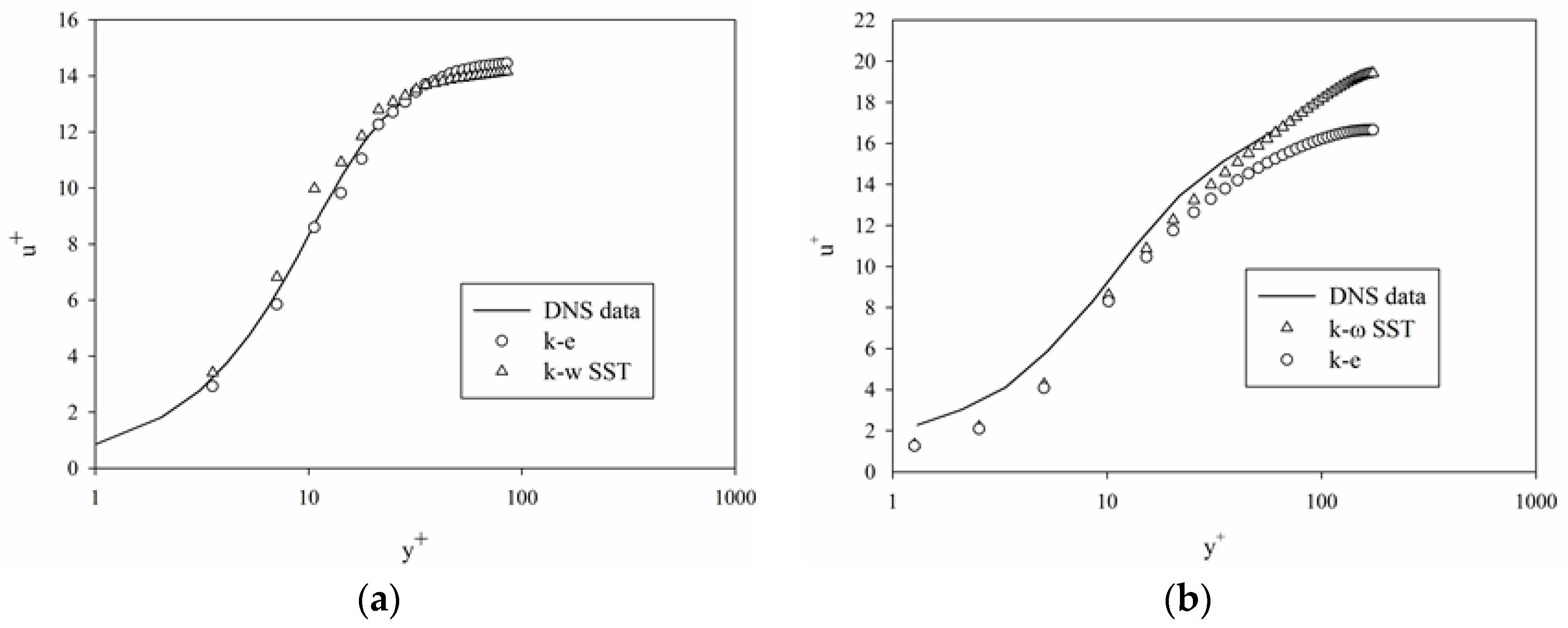
3.2.3. Turbulence Model

To justify the use of k-ε and k-ω SST models, we compared simulation results with Direct Numerical Simulation (DNS) data obtained from the literature in closely related flows. The turbulence k-ε model is a semi-empirical Reynolds-Averaged Navier-Stokes (RANS) model that solves model transport equations for the turbulent kinetic energy, k, and the turbulent kinetic energy dissipation rate, ε [42]. The k-ε model is the most commonly used turbulence model, available in most commercial CFD codes [48]. Some of the advantages of the k-ε model are robustness, reasonable accuracy for wide flow ranges, and computational economy [1,3]. The k-ε model has been commonly used to design prosthetic heart devices [49,50,51,52,53,54]. For the k-ω turbulence model, the shear-stress transport (SST) k-ω model was used. This is the second most commonly used two-equation model after the k-ε model [48]. The k-ω SST model solves the model transport equations for turbulent kinetic energy, k and ω which is defined as $\mathsf{\omega }\equiv \frac{\mathsf{\epsilon }}{k}$ [42]. Both models solve the same equation for the turbulence kinetic energy and they differ when solving the second variable. The k-ω model is considered to be more accurate for flow field predictions at low Reynolds number flows and in the viscous near-wall region when solving boundary-layer flows. However, it has difficulty when solving non-turbulent free-stream boundaries [48]. Also, the k-ω SST model has commonly been used to design prosthetic heart devices [18,55,56,57,58]. In this study, the turbulence models have been used with the enhanced wall treatments available in Fluent to resolve near wall flow conditions.

As already mentioned, the choice of the turbulence models was decided by comparing simulation results with the DNS obtained from literature [59,60]. Both Couette viscometer and capillary tube experiments were simulated by using both k-ε and k-ω SST turbulence models. The simulation results and the DNS data were matched at corresponding friction Reynolds number, Re_τ, which was defined as ${\mathrm{Re}}_{\mathsf{\tau }}=\frac{R}{l^{*}}$ where R is the radius of the pipe and l^* is the viscous length scale in wall turbulence. In the case of Couette viscometer, Re_τ was defined as ${\mathrm{Re}}_{\mathsf{\tau }}=\frac{uh/2}{\nu }$. Couette viscometer simulations were performed with both k-ε and k-ω SST models until obtaining Re_τ value that was given in the DNS data [60]. In the case of capillary tube, simulations were performed at Re_τ matching the DNS data of Chin et al. [59]. After simulations were performed, the mean velocity profiles for the near-wall regions were calculated using the dimensionless wall parameters. The dimensionless distance from the wall, $y^{+}$, was calculated based on distance from wall, Y, and viscous length scale, $l^{*}$, as $y^{+}=\frac{Y}{l^{*}}$. The dimensionless velocity, u⁺, was calculated as $u^{+}=\frac{\langle U\rangle }{u^{*}}$, where $\langle U\rangle$ is the mean velocity. The mean velocity profile for the Couette viscometer is plotted with the DNS data in Figure 3a [60]. It can be seen from Figure 3a that using either the k-ε or the k-ω SST model in the computation of the flow domain did not show significant differences. After determination of the root mean square error for both models, the k-ε model was selected for simulation of the Couette experiments (

Table 3. Root mean square errors for the Couette viscometer [16] and capillary tube experiments [4].

Root Mean Square Error	Couette Viscometer	Capillary Tube
k-ε Model	0.39	1.32
k-ω SST Model	0.65	1.04

). The mean velocity profile for the capillary tube is shown in Figure 3b. Based on error calculations, the k-ω SST model was chosen for the capillary tube simulations (Table 3).

3.2.4. Reynolds Stress Calculation

Reynolds stress calculations were performed for both flow configurations at a post-processing stage. For both capillary tube and Couette viscometer experiments several lines (called rakes in FLUENT) were created with multiple points through the model geometry. Rakes were created equally spaced and each rake had several points that were equally spaced. Then, Reynolds stresses were calculated in each point of each rake and eventually there were more than 1000 different calculated Reynolds stress values for both capillary tube and Couette viscometer. For the capillary tube, the rakes were created through the narrow part of the capillary tube seen in Figure 1b. Time-averaged velocity gradients at each point of every rake (${\mathsf{\tau }}_{\nu }=\mathsf{\mu }\frac{d{\overline{u}}_x}{dy}$ on rakes aligned with the y-axis and ${\mathsf{\tau }}_{\nu }=\mathsf{\mu }\frac{d{\overline{u}}_x}{dz}$ along rakes aligned in the z-axis) yielded viscous stresses. The total stress, ${\mathsf{\tau }}_t=\frac{r}{R}{\mathsf{\tau }}_w$, was found at each point and the Reynolds stresses were calculated by taking the difference between viscous and total stresses ${\mathsf{\tau }}_{\mathrm{Re}}={\mathsf{\tau }}_t-{\mathsf{\tau }}_{\nu }$. Finally, the area-averaged Reynolds stress, <τ_Re>, was calculated by using

$$\langle {\mathsf{\tau }}_{\mathrm{Re}}\rangle =\frac{{\displaystyle \sum _{i=1}^{N_{bins}}{\mathsf{\tau }}_{{\mathrm{Re}}_{r_i}}\mathsf{\pi }\left(r_i^2-r_{i-1}^2\right)}}{\mathsf{\pi }{R}^2},$$

(15)

where ${\mathsf{\tau }}_{{\mathrm{Re}}_{r_i}}$ is the Reynolds stress at point r_i, N_bins, is the number of points in each rake, and r_i is the distance of each point from the center of the capillary tube. For the Couette viscometer, rakes were created in the yellow vertical plane shown in Figure 1a. Calculations of viscous stresses, Reynolds stresses, and area-averaged Reynolds stresses were conducted similarly to the capillary tube, keeping in mind that the total stresses for the Couette viscometer were calculated as

$${\mathsf{\tau }}_{r\mathsf{\theta }}=2\mathsf{\mu }{\mathsf{\Omega }}_i\frac{R_i^2{R}_o^2}{\left(R_o^2-R_i^2\right)}\left(\frac{1}{r^2}\right),$$

(16)

where, ${\mathsf{\Omega }}_i$ is the rotation rate of the inner cylinder, $R_i$ is the radius of the inner cylinder and $R_o$ is the radius of the outer cylinder.

4. Results and Discussion

It is assumed that the simulated systems were well mixed in turbulent flow. Therefore, cells are assumed to spend on average the same amount of time in any location inside of the flow field. Four different power law models [10,11,18,23] were used to investigate the effect of time-averaged and area-averaged Reynolds, in addition to total, viscous and wall shear stresses to hemolysis.

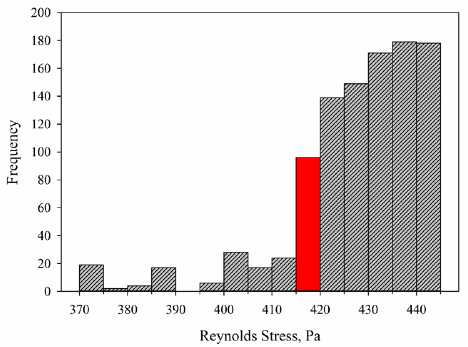
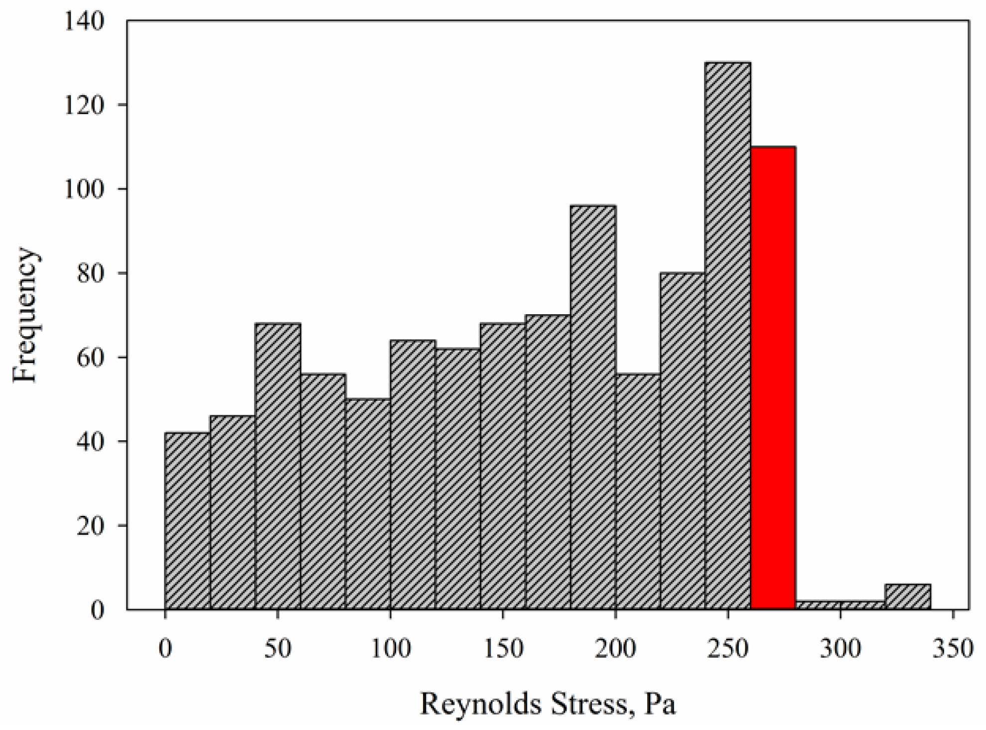
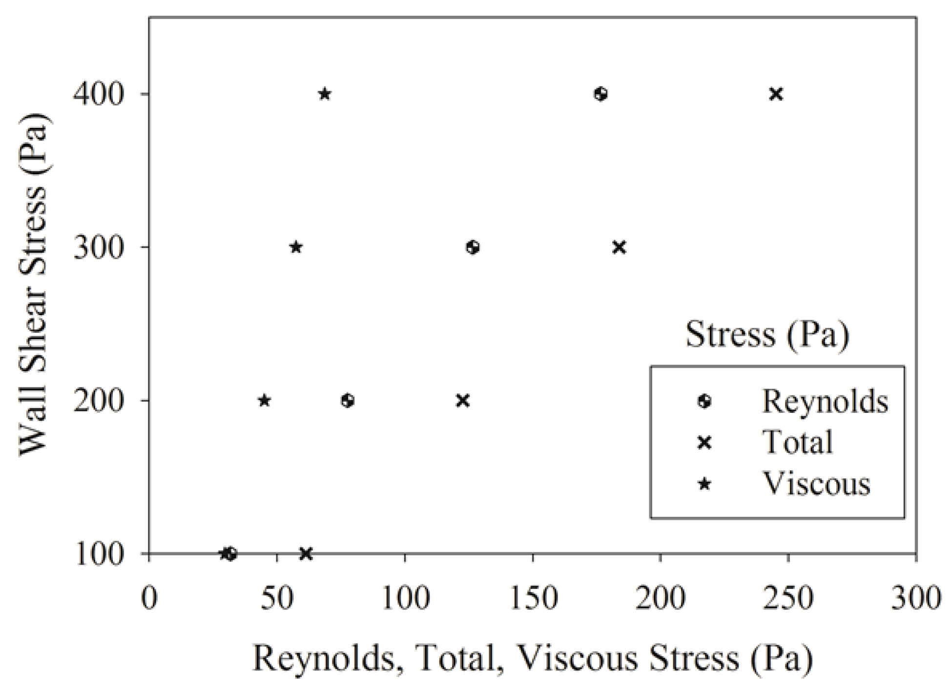
4.1. Reynolds Stress Distributions in Couette Viscometer

Simulations were performed for seven experiments of the Couette viscometer [16] as seen in Table 1. With varying amounts of hemolysis levels (1%–85%) using the Couette viscometer, exploring the existence of a critical (or threshold) value provided a unique perspective on the importance of Reynolds and viscous stresses for hemolysis. Experimental % hemolysis values were obtained from the original work of Sutera and Mehrjardi [16] (Table 1). The spatial distributions of Reynolds stresses (RS) were found for each experiment of the Couette viscometer. Contours of constant stress were mapped for a given experiment and the threshold RS was taken to be on the contour corresponding to the contour level enclosing a volume percent of the flow domain equal to the percent hemolysis. A histogram of results (Figure 4) showed that for the highest shear stress experiment (450 Pa), the threshold RS value was found to be 417 Pa (shown with red color in Figure 4), which means that 85% (hemolysis level of 450 Pa experiment) of the spatial distribution of RS was above this value. When the next highest shear stress experiment (350 Pa) was observed, it was seen that the threshold RS value was 336 Pa, which is lower than the threshold value of the previous experiment. The same analysis was repeated for the entire sequence of lower shear rate experiments (all of the frequency plots are not shown here for brevity) and it was found that the threshold Reynolds stresses shifted continually toward the lower end of the frequency plots. Threshold Reynolds stress values for the other six experiments (350–50 Pa) changed from 336 to 49 dynes/cm². While these experiments were all run at 4 min duration, we note that the times that cells spent in regions of high shear stress may have varied from one experiment to the other.

When all the threshold RS values were compared for Couette viscometer, it can be seen that results (Figure 5) for Reynolds stress threshold values stretched over an order of magnitude. If Reynolds stress was critical for hemolysis, one might expect there to be a common value above which hemolysis is found, given that the exposure time of the RBCs in the Couette viscometer experiments was 4 min. However, results showed that there was not a critical RS leading to hemolysis. For example, for the 200 Pa experiment, the critical RS value was 196 Pa. However, in the 150 Pa experiment, the critical RS value was 147 Pa. If we rely on the 200 Pa experiment, we accept the threshold RS value for hemolysis to be 196 Pa. When we look at the 150 Pa experiment, we would expect that there should not be any hemolysis at 150 Pa. When the other experiments are considered in the same way, it can be seen that there is not a common value of critical RS for all experiments.

4.2. Viscous Stress Distributions in Couette Viscometerr

Viscous stress threshold analysis for the Couette viscometer was performed the same way as the RS threshold analysis. Viscous stress calculation does not contain viscous stresses in or between turbulent structures. They were calculated from time-averaged velocity gradients on several locations in the domain from ${\mathsf{\tau }}_{\nu }=\mathsf{\mu }\frac{d{\overline{u}}_x}{dy}$ on rakes aligned with the y-axis and ${\mathsf{\tau }}_{\nu }=\mathsf{\mu }\frac{d{\overline{u}}_x}{dz}$ along rakes aligned in the z-axis. For each experiment of the Couette viscometer, the distribution of viscous stresses was found (histogram was not shown here for brevity). Then, depending on the hemolysis level of each experiment, the threshold viscous stresses were found. When all the threshold viscous stress values are compared for Couette viscometer, it can be seen that viscous stress threshold values are also different for each experiment (Figure 6). As in the RS, if viscous stress were critical for hemolysis, there would be a common value for a critical viscous stress above which hemolysis occurs. It should further be noted that these stress levels are below thresholds known for laminar flow experiments.

The threshold analysis of both RS and viscous stress showed that threshold stresses were changing in each different experiment of Couette viscometer.

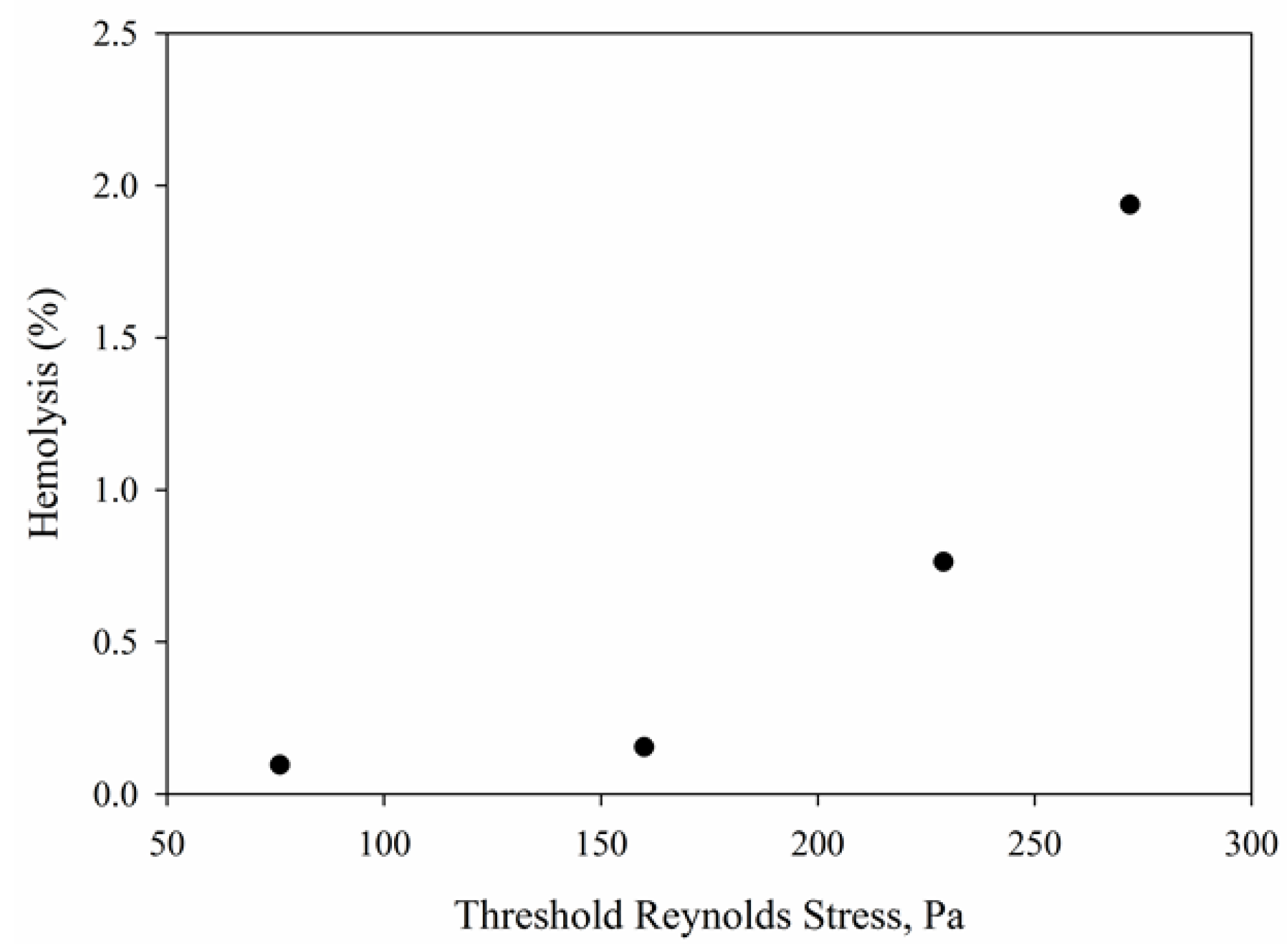
4.3. Reynolds Stress Distributions in Capillary Tube

Simulations were performed for four capillary tube experiments as seen in Table 2. Although capillary tube experiments have lower degrees of hemolysis than these for Couette viscometer, they still have varying levels of hemolysis for each experiment. Hemolysis levels varied from 0.1% to 1.9% enabling threshold analysis in the same way as in the Couette viscometer. Experimental % hemolysis values were not provided directly in the original work [4]. We calculated hemolysis using the formula $H(\%)=\frac{\mathrm{\Delta }{H}_b}{H_b}100$ where H is the percentage of hemolysis, $\mathrm{\Delta }{H}_b$ is change of plasma hemoglobin as hemoglobin is released, and Hb is the total amount of hemoglobin [10] (hemolysis values can be seen in Table 2). Results show that for the highest shear stress experiment (400 Pa), the threshold RS value is 272 Pa (shown with red color in Figure 7), representing that 1.9% (hemolysis level of 400 Pa experiment) of spatial distribution of RS was above this value.

In the next highest shear stress experiment (300 Pa), it was seen that the threshold RS value decreased to 229 Pa. Similar analyses were repeated for the lower shear rate experiments (not all of the frequency plots are shown here for brevity). The threshold RS values for each experiment showed that there were four different Reynolds stress threshold values for four different experiments (Figure 8). As in Couette viscometer experiments, it was expected to see a common threshold. Results do not support RS as a determining factor for hemolysis.

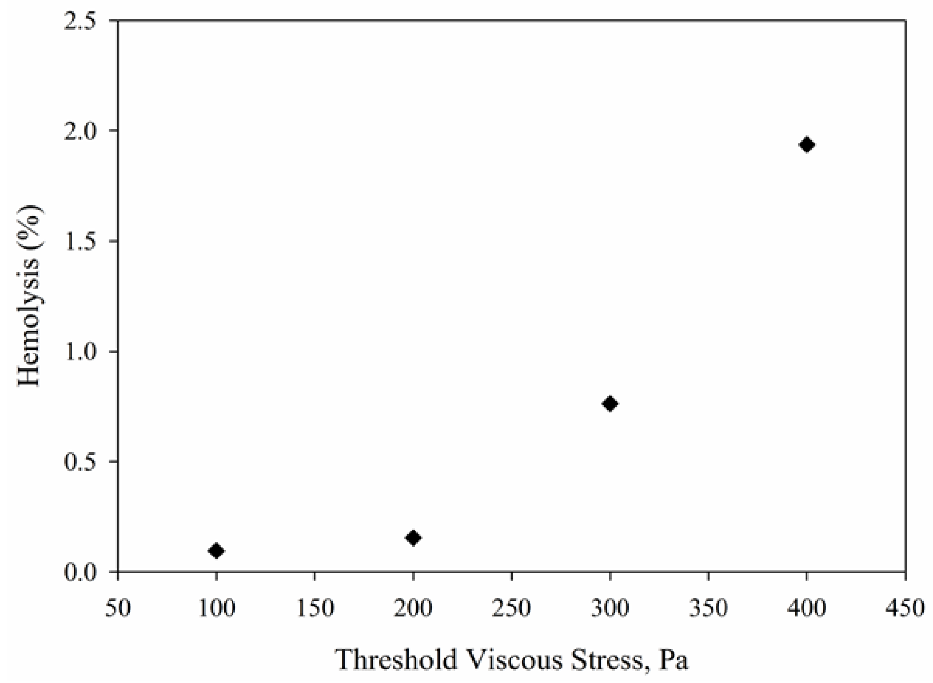
4.4. Viscous Stress Distributions in Capillary Tube

A similar procedure was applied to viscous stresses for the capillary tube. Viscous stress distributions were calculated for each experiment of the capillary tube (frequency plots are not shown for brevity) and threshold viscous stresses determined (Figure 9). Threshold viscous stress increased with increasing shear stress with no common viscous stress value found for the capillary tube.

It can be concluded as a result of RS and viscous stress threshold analysis for the experiments of capillary tube that both time-averaged, area-averaged RS and viscous stresses are not determining parameters for hemolysis.

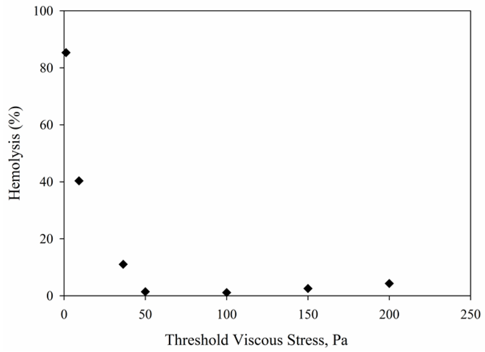
4.5. Hemolysis Calculations Using Power Models

In the previous section, it was seen that RS and viscous stress do not exhibit a threshold value for hemolysis. In order to explore this question further, we have used commonly accepted power law models [10,11,18,23] in the form of Equation (1) to investigate the effects of area-averaged, time-averaged RS, viscous, total, and wall shear stresses on hemolysis (see

Table 4. Calculated Hemolysis Index (HI) applying four different and commonly used power law models and standard error when calculations are compared to experimental measurements by Kameneva et al. [4] ¹.

Power Law Models	Type of Stress	Calculated HI for τw = 100 Pa	Calculated HI for τw = 200 Pa	Calculated HI for τw = 300 Pa	Calculated HI for τw = 400 Pa	Standard Error [24]
Experimental Hemolysis Data [4]	τw	0.0954	0.1538	0.7625	1.9375	0
Giersiepen et al. [23] $HI(\%)=3.62\times {10}^{-5}{\mathsf{\tau }}^{2.416}{t}^{0.785}$	τRe	0.4106	3.9302	13.8268	32.0492	6.6658
	τt	2.0132	11.8869	34.1216	70.8037	14.8321
	τv	0.3455	1.0587	2.0452	3.2602	0.2485
	τw	6.5674	38.7766	111.3085	230.9699	49.3428
Heuser et al. [10] $HI(\%)=1.8\times {10}^{-6}{\mathsf{\tau }}^{1.991}{t}^{0.765}$	τRe	0.0051	0.0335	0.0963	0.1944	0.3861
	τt	0.0188	0.0833	0.2028	0.3735	0.3513
	τv	0.0044	0.0114	0.0199	0.0296	0.4224
	τw	0.0497	0.2208	0.5372	0.9897	0.2126
Zhang et al. [11] $HI(\%)=1.228\times {10}^{-5}{\mathsf{\tau }}^{1.9918}{t}^{0.6606}$	τRe	0.0514	0.3568	1.065	2.1868	0.0557
	τt	0.1905	0.8886	2.2428	4.2034	0.469
	τv	0.0445	0.121	0.2203	0.3323	0.3686
	τw	0.5049	2.3553	5.9447	11.1413	1.9226
Fraser et al. [18] $HI(\%)=1.745\times {10}^{-6}{\mathsf{\tau }}^{1.963}{t}^{0.7762}$	τRe	0.0043	0.0274	0.0775	0.1546	0.3947
	τt	0.0155	0.0673	0.1614	0.2943	0.3677
	τv	0.0037	0.0094	0.0164	0.0241	0.4234
	τw	0.0406	0.176	0.4217	0.7692	0.267

¹ In Table 4, HI is the hemolysis index, τ is the shear stress (Pa), t is exposure time (s), τ_Re, τ_t, τ_v, and τ_w are average RS, total, viscous, and wall shear stresses (Pa), to indicate which is used as τ in the power law models.

).

The standard error between experimental hemolysis data and theoretical calculation is also found for the experiments in capillary tube and is shown in Table 4. (Power law models are not expected to apply to the Couette viscometer experiments, because they were conducted for the very long RBC exposure time of 4 min). Standard error (SE) calculation [24] was performed using the formula $SE=\frac{sdev}{\sqrt{N}}$ where sdev is the standard deviation and N is the number of observations that correspond to the four different experiments of Kameneva et al. [4]. Hemolysis predictions show that the power law model of Zhang [11] gives the lowest standard error. The highest error was obtained by using Giersiepen’s [23] power law model. When results were compared examining different stresses (RS, viscous, total, and wall shear stresses), the best agreement between the experimental data and the power law models was obtained by using RS. The worst agreement was obtained by using wall shear stress with Giersiepen’s [23] power law model. The greater error is expected because 300 and 400 Pa are outside the range of the experimental conditions used to obtain Giersiepen’s model (stresses were less than 255 Pa and exposure times were less than 700 ms). Even though the 400 Pa experiment was higher than the experimental shear stress of Zhang’s model (exposure times of less than 1500 ms and shear stresses between 50–320 Pa), it still gave the smallest error with RS. Zhang’s model is applicable to much lower shear stresses than experimental conditions of Kameneva but it still gave smaller errors compared to Fraser and Heuser. These calculations illustrate the challenge in applying the power law models developed from homogeneous laminar flow measurement to the analysis of devices with complex turbulent flows.

One of the most significant findings of Kameneva et al. [4] was that turbulent and laminar flows with equal shear stress at the wall resulted in very different blood trauma. There are factors, therefore, in addition to wall shear stress that contribute to increasing hemolysis for turbulent flow conditions. The turbulence feature that leads to RBC trauma cannot be the Reynolds stresses acting the way viscous stresses act in laminar flows. Area-averaged RSs, total and viscous stresses are plotted for the capillary tube in Figure 10. It is found that the Reynolds stresses in a turbulent flow with the same wall shear stress as in laminar flow are in fact smaller than the laminar flow shear stresses (when they were both area averaged). It is obvious from Figure 10 that Reynolds stress is less in magnitude than the total stress for the same wall shear stress.

Moreover, viscous stress is the smallest when compared to Reynolds and total stress for the same wall shear stress.

5. Conclusions

The lack of a fundamental physical description of the hemolysis mechanisms in a turbulent flow field complicates a deterministic approach to hemolysis prediction. There is a need to clarify the effect of different stresses in hemolysis. In this work, a threshold analysis for Reynolds stress (RS) and viscous stress was examined for a Couette viscometer and a capillary tube by assuming that systems were well mixed and cells on average spent the same amount of time in any location inside the flow field. While these experiments provide data on hemolysis under well-defined conditions, they do not represent the clinical situation in reproducing flow history or by employing non-physiological hematocrits (i.e., much less than the 40%–55% range), and washed cells and porcine blood. Results of simulations under the conditions of these Couette and capillary experiments showed that there is not a common threshold value for Reynolds and viscous stress where hemolysis happens. It is worth noting on consideration of Leverett’s shear stress-exposure time plot that, under certain conditions, an exposure time threshold might be more appropriate.

Therefore, it is evident that neither Reynolds nor viscous stress is a good predictor when determining hemolysis. At present, additional investigation of threshold analysis of Reynolds and viscous stresses in other devices and systems is required to confirm widespread applicability of these findings. At this time, the threshold analysis may offer insight into the hemolysis calculations by using Reynolds and viscous stresses.

When applying a power law model that takes into account stress and exposure time of the red blood cells (RBCs), use of the RS rather than the total stresses or the viscous stresses in the power law formula is found to provide better agreement between model and measurements at least in both systems modeled. However, it appears the coefficients of the power law formulation must be empirically derived for each device. This is a disadvantage of this class of hemolysis models.

References

1. Fraser, K.H.; Taskin, M.E.; Griffith, B.P.; Wu, Z.J. The use of computational fluid dynamics in the development of ventricular assist devices. Med. Eng. Phys. 2011, 33, 263–280. [Google Scholar] [CrossRef] [PubMed]
2. Antiga, L.; Steinman, D.A. Rethinking turbulence in blood. Biorheology 2009, 46, 77–81. [Google Scholar] [PubMed]
3. Hund, S.J.; Antaki, J.F.; Massoudi, M. On the representation of turbulent stresses for computing blood damage. Int. J. Eng. Sci. 2010, 48, 1325–1331. [Google Scholar] [CrossRef] [PubMed]
4. Kameneva, M.V.; Burgreen, G.W.; Kono, K.; Repko, B.; Antaki, J.F.; Umezu, M. Effects of turbulent stresses upon mechanical hemolysis: Experimental and computational analysis. ASAIO J. 2004, 50, 418–423. [Google Scholar] [CrossRef] [PubMed]
5. Aziz, A.; Werner, B.C.; Epting, K.L.; Agosti, C.D.; Curtis, W.R. The cumulative and sublethal effetcs of turbulence on erythrocytes in a stirred-tank model. Ann. Biomed. Eng. 2007, 35, 2108–2120. [Google Scholar] [CrossRef] [PubMed]
6. Bludszuweit, C. Three-dimensional numerical prediction of stress loading of blood particles in a centrifugal pump. Artif. Organs. 1995, 19, 590–596. [Google Scholar] [CrossRef] [PubMed]
7. Leverett, L.B.; Hellums, J.D.; Alfrey, C.P.; Lynch, E.C. Red blood cell damage by shear stress. Biophys. J. 1972, 12, 257–273. [Google Scholar] [CrossRef]
8. Blackshear, P.L. Mechanical Hemolysis in Flowing Blood; Prentice-Hall: Englewood Cliffs, NJ, USA, 1972. [Google Scholar]
9. Grigioni, M.; Daniele, C.; Morbiducci, U.; D’Avenio, G.; Benedetto, G.D.; Barbaro, V. The power-law mathematical model for blood damage prediction: Analytical developments and physical inconsistencies. Artif. Organs 2004, 28, 467–475. [Google Scholar] [CrossRef] [PubMed]
10. Heuser, G.; Opitz, R. A Couette viscometer for short time shearing of blood. Biorheology 1980, 17, 17–24. [Google Scholar] [PubMed]
11. Zhang, T.; Taskin, M.E.; Fang, H.B.; Pampori, A.; Jarvik, R.; Griffith, B.P.; Wu, Z.J. Study of flow-induced hemolysis using novel Couette-type blood shearing devices. Artif. Organs 2011, 35, 1180–1186. [Google Scholar] [CrossRef] [PubMed]
12. Marom, G.; Bluestein, D. Lagrangian methods for blood damage estimation in cardiovascular devices—How numerical implementation affects the results. Expert Rev. Med. Devices 2016, 13, 113–122. [Google Scholar] [CrossRef] [PubMed]
13. Sheriff, J.; Soares, J.S.; Xenos, M.; Jesty, J.; Bluestein, D. Evaluation of shear-induced platelet activation models under constant and dynamic shear stress loading conditions relevant to devices. Ann. Biomed. Eng. 2013, 41, 1279–1296. [Google Scholar] [CrossRef] [PubMed]
14. Soares, J.S.; Sheriff, J.; Bluestein, D. A novel mathematical model of activation and sensitization of platelets subjected to dynamic stress histories. Biomech. Model. Mechanobiol. 2013, 12, 1127–1141. [Google Scholar] [CrossRef] [PubMed]
15. Goubergrits, L. Numerical modeling of blood damage: Current status, challenges and future prospects. Expert Rev. Med. Devices 2006, 3, 527–531. [Google Scholar] [CrossRef] [PubMed]
16. Sutera, S.P.; Mehrjardi, M.H. Deformation and fragmentation of human red blood cells in turbulent shear flow. Biophys. J. 1975, 15, 1–10. [Google Scholar] [CrossRef]
17. Burgreen, G.W.; Antaki, J.F.; Wu, Z.J.; Holmes, A.J. Computational fluid dynamics as a development tool for rotary blood pumps. Artif. Organs 2001, 25, 336–340. [Google Scholar] [CrossRef] [PubMed]
18. Fraser, K.H.; Zhang, T.; Taskin, M.E.; Griffith, B.P.; Wu, Z.J. A quantitative comparison of mechanical blood damage parameters in Rotary Ventricular Assist Devices: Shear stress, exposure time, and hemolysis index. J. Biomech. Eng. 2012, 134, 081002. [Google Scholar] [CrossRef] [PubMed]
19. Izraelev, V.; Weiss, W.J.; Fritz, B.; Newswanger, E.; Paterson, G.; Snyder, A.; Medvitz, R.B.; Cysyk, J.; Pae, W.E.; Hicks, D.; et al. A passively suspended Tesla pump left ventricular assist device. Am. Soc. Artif. Intern. Organs 2009, 55, 556–561. [Google Scholar] [CrossRef] [PubMed]
20. Morsi, Y.S.; Yang, W.; Witt, P.J.; Ahmed, A.M.; Umezu, M. Numerical analysis of the flow characteristics of rotary blood pump. J. Artif. Organs 2001, 4, 54–60. [Google Scholar] [CrossRef]
21. Nguyen, V.T.; Kuan, Y.H.; Chen, P.Y.; Ge, L.; Sotiropolous, F.; Yoganathan, A.P.; Leo, H.L. Experimentally validated hemodynamics simulations of mechanical heart valves in three dimensions. Cardiovasc. Eng. Technol. 2012, 3, 88–100. [Google Scholar] [CrossRef]
22. Wu, J.; Paden, B.E.; Borovetz, H.S.; Antaki, J.F. Computational fluid dynamics analysis of blade tip clearances on hemodynamic performance and blood damage in a centrifugal ventricular assist device. Artif. Organs 2010, 34, 402–411. [Google Scholar] [CrossRef] [PubMed]
23. Giersiepen, M.; Wurzinger, L.J.; Opitz, R.; Reul, H. Estimation of shear stress-related blood damage in heart valve prostheses-in vitro comparison of 25 aortic valves. Int. J. Artif. Organs 1990, 13, 300–306. [Google Scholar] [PubMed]
24. Chapra, S.C.; Canale, R.P. Numerical Methods for Engineers; McGraw-Hill: New York, NY, USA, 2010. [Google Scholar]
25. Ozturk, M.; O’Rear, E.A.; Papavassiliou, D.V. Hemolysis related to turbulent eddy size distributions using comparisons of experiments to computations. Artif. Organs 2015, 39, E227–E239. [Google Scholar] [CrossRef] [PubMed]
26. Vitale, F.; Nam, J.; Turchetti, L.; Behr, M.; Raphael, R.; Annesini, M.C.; Pasquali, M. A multiscale, biophysical model of flow-induced red blood cell damage. Am. Inst. Chem. Eng. J. 2014, 60, 1509–1516. [Google Scholar] [CrossRef]
27. Quinlan, N.J.; Dooley, P.N. Models of flow-induced loading on blood cells in laminar and turbulent flow, with application to cardiovascular device flow. Ann. Biomed. Eng. 2007, 35, 1347–1356. [Google Scholar] [CrossRef] [PubMed]
28. Liu, J.S.; Lu, P.C.; Chu, S.H. Turbulence characteristics downstream of bileaflet aortic valve protheses. J. Biomech. Eng. 1999, 122, 118–124. [Google Scholar] [CrossRef]
29. Li, C.P.; Lo, C.W.; Lu, P.C. Estimation of viscous dissipative stresses induced by a mechanical heart valve using PIV data. Ann. Biomed. Eng. 2010, 38, 903–916. [Google Scholar] [CrossRef] [PubMed]
30. Quinlan, N.J. Mechanical Loading of Blood Cells in Turbulent Flow; Springer: New York, NY, USA, 2014. [Google Scholar]
31. Yen, J.H.; Chen, S.F.; Chern, M.K.; Lu, P.C. The effect of turbulent viscous shear stress on red blood cell hemolysis. J. Artif. Organs 2014, 17, 178–185. [Google Scholar] [CrossRef] [PubMed]
32. Lee, H.; Tatsumi, E.; Taenaka, Y. Experimental study on the Reynolds and viscous shear stress of bileaflet mechanical heart valves in a pneumatic ventricular assist device. ASAIO J. 2009, 55, 348–354. [Google Scholar] [CrossRef] [PubMed]
33. Jones, S.A. A relationship between reynolds stresses and viscous dissipation: Implications to red cell damage. Ann. Biomed. Eng. 1995, 23, 21–28. [Google Scholar] [CrossRef] [PubMed]
34. Sallam, A.M.; Hwang, N.H.C. Human red blood cell hemolysis in a turbulent shear flow: Contribution of Reynolds shear stresses. Biorheology 1984, 21, 783–797. [Google Scholar] [PubMed]
35. Sallam, A.M. An Investigation of the Effect of Reynolds Shear Stress on Red Blood Cell Hemolysis. Ph.D. Thesis, University of Houston, Houston, TX, USA, 1982. [Google Scholar]
36. Sallam, A.M.; Hwang, N.H.C. Influence of red blood cell concentrations on the measurement of turbulence using hot-film anemometer. J. Biomech. Eng. 1983, 105, 406–410. [Google Scholar] [CrossRef] [PubMed]
37. Ellis, J.T.; Wick, T.M.; Yoganathan, A.P. Prosthesis-induced hemolysis: Mechanisms and quantification of shear stress. J. Heart Valve Dis. 1998, 7, 376–386. [Google Scholar] [PubMed]
38. Grigioni, M.; Caprari, P.; Tarzia, A.; D’Avenio, G. Prosthetic heart valves’ mechanical loading of red blood cells in patients with hereditary membrane defects. J. Biomech. 2005, 38, 1557–1565. [Google Scholar] [CrossRef] [PubMed]
39. Boehning, F.; Mejia, T.; Schmitz-Rode, T.; Steinseifer, U. Hemolysis in a laminar flow-through Couette shearing device: An experimental study. Artif. Organs 2014, 38, 761–765. [Google Scholar] [CrossRef] [PubMed]
40. Paul, R.; Apel, J.; Klaus, S.; Schugner, F.; Schwindke, P.; Reul, H. Shear stress related blood damage in laminar couette flow. Artif. Organs 2003, 27, 517–529. [Google Scholar] [CrossRef] [PubMed]
41. Bacher, R.P.; Williams, M.C. Hemolysis in capillary flow. J. Lab. Clin. Med. 1970, 76, 485–496. [Google Scholar] [PubMed]
42. ANSYS Inc. ANSYS Fluent 14.0: Theory Guide; ANSYS Inc.: Canonsburg, PA, USA, 2011. [Google Scholar]
43. Ge, L.; Dasi, L.P.; Sotiropolous, F.; Yoganathan, A.P. Characterization of hemodynamic forces induced by mechanical heart valves: Reynolds vs. viscous stresses. Ann. Biomed. Eng. 2008, 36, 276–297. [Google Scholar] [CrossRef] [PubMed]
44. Puri, A.N.; Kuo, C.Y.; Chapman, R.S. Turbulent diffusion of mass in circular pipe flow. Appl. Math. Model. 1983, 7, 135–138. [Google Scholar] [CrossRef]
45. Roberts, P.J.W.; Webster, D.R. Turbulent Diffusion. In Environmental Fluid Mechanics: Theories and Applications; Shen, H.H., Ed.; American Society of Civil Engineers: Reston, VA, USA, 2002. [Google Scholar]
46. Bird, R.B.; Stewart, W.E.; Lightfoot, E.N. Transport Phenomena, 2nd ed.; John Wiley & Sons, Inc.: New York, NY, USA, 2002. [Google Scholar]
47. Davidson, P.A. Turbulence: An Introduction for Scientists and Engineers; Oxford University Press: New York, NY, USA, 2004. [Google Scholar]
48. Pope, S.B. Turbulent Flows; Cambridge University Press: New York, NY, USA, 2000. [Google Scholar]
49. Apel, J.; Neudel, F.; Reul, H. Computational fluid dynamics and experimental validation of a microaxial blood pump. ASAIO J. 2001, 47, 552–558. [Google Scholar] [CrossRef] [PubMed]
50. Chua, L.P.; Song, G.; Yu, S.C.M.; Lim, T.M. Computational fluid dynamics of gap flow in a biocentrifugal blood pump. Artif. Organs 2005, 29, 620–628. [Google Scholar] [CrossRef] [PubMed]
51. Mitoh, A.; Yano, T.; Sekine, K.; Mitamura, Y.; Okamoto, E.; Kim, D.W.; Yozu, R.; Kawada, S. Computational fluid dynamics analysis of an intra-cardiac axial flow pump. Artif. Organs 2003, 27, 34–40. [Google Scholar] [CrossRef] [PubMed]
52. Schenkel, A.; Deville, M.O.; Sawley, M.L. Flow simulation and hemolysis modeling for a blood centrifuge device. Comput. Fluids 2013, 86, 185–198. [Google Scholar] [CrossRef]
53. Yano, T.; Sekine, K.; Mitoh, A.; Mitamura, Y.; Okamoto, E.; Kim, D.W.; Nishimura, I.; Murabayashi, S.; Yozu, R. An estimation method of hemolysis within an axial flow blood pump by computational fluid dynamics analysis. Artif. Organs 2003, 27, 920–925. [Google Scholar] [CrossRef] [PubMed]
54. Zhang, Y.; Zhan, Z.; Gui, X.M.; Sun, H.S.; Zhang, H.; Zheng, Z.; Zhou, J.Y.; Zhu, X.D.; Li, G.R.; Hu, S.S.; et al. Design optimization of an axial blood pump with computational fluid dynamics. ASAIO J. 2008, 54, 150–155. [Google Scholar] [CrossRef] [PubMed]
55. Al-Azawy, M.; Turan, A.; Revell, A. Investigating the use of turbulence models for flow investigations in a positive displacement ventricular assist devices. In Proceedings of the 6th European Conference of the International Federation for Medical and Biological Engineering, Dubrovnik, Croatia, 7–11 September 2014; pp. 395–398.
56. Carswell, D.; McBride, D.; Croft, N.; Slone, A.; Croft, N.; Foster, G. A CFD model for the prediction of haemolysis in micro axial left ventricular assist devices. Appl. Math. Model. 2013, 37, 4199–4207. [Google Scholar] [CrossRef]
57. Kido, K.; Hoshi, H.; Watanabe, N.; Kataoka, H.; Ohuchi, K.; Asama, J.; Shinshi, T.; Yoshikawa, M.; Takatani, S. Computational fluid dynamics analysis of the Pediatric tiny centrifugal blood pump (TinyPump). Artif. Organs 2006, 30, 392–399. [Google Scholar] [CrossRef] [PubMed]
58. Song, X.; Wood, H.G.; Day, S.W.; Olsen, D.B. Studies of turbulence models in a computational fluid dynamics model os a blood pump. Artif. Organs 2003, 27, 935–937. [Google Scholar] [CrossRef] [PubMed]
59. Chin, C.; Monty, J.P.; Ooi, A. Reynols number effects in DNS of pipe flow and comparison with channels and boundary layers. Int. J. Heat Fluid Flow 2014, 45, 33–40. [Google Scholar] [CrossRef]
60. Pirro, D.; Quadrio, M. Direct numerical simulation of turbulent Taylor-Couette flow. Eur. J. Mech. B Fluids 2008, 27, 552–566. [Google Scholar] [CrossRef]
Figure 1. (a) 3D computational model of 1/32nd of the viscometer used in Sutera and Mehrjardi [16]; (b) 3D model of the capillary tube used in Kameneva et al. [4].
Fluids 01 00042 g001
Figure 2. Determination of cell count for grid independence: (a) Grid independence analysis for Couette viscometer for highest shear stress (450 Pa) experiment by using k-ε model (Bottom row in Table 1); (b) grid independence analysis for capillary tube for the highest shear stress (400 Pa) experiment by using k-ω SST model (Bottom row in Table 2).
Fluids 01 00042 g002
Figure 3. (a) Couette viscometer mean velocity profiles near wall for the DNS data of Pirro et al. [60]: solid line, k-ε model: circles, k-ω SST model: triangles; (b) capillary tube mean velocity profiles near wall for the DNS data of Chin et al. [59]: solid line, k-ε model: circles, k-ω SST model: triangles.
Fluids 01 00042 g003
Figure 4. Frequency of Reynolds stresses in Couette viscometer for 450 Pa. The frequency and experimentally observed hemolysis of 85% suggest a threshold of 417 Pa.
Fluids 01 00042 g004
Figure 5. Relationship of hemolysis to threshold Reynolds stresses in Couette viscometer for all experiments (450 to 50 Pa).
Fluids 01 00042 g005
Figure 6. Relationship of hemolysis to threshold viscous stresses in Couette viscometer for all experiments (450 to 50 Pa).
Fluids 01 00042 g006
Figure 7. Frequency of Reynolds stresses in capillary tube for the case whereby τ w = 400   Pa .
Fluids 01 00042 g007
Figure 8. Relationship of hemolysis to threshold Reynolds stresses in capillary tube for all of the experiments (100 to 400 Pa).
Fluids 01 00042 g008
Figure 9. Relationship of hemolysis to threshold viscous stresses in capillary tube for all experiments (400 to 100 Pa).
Fluids 01 00042 g009
Figure 10. Changes of area-averaged Reynolds, total, and viscous stress with four different wall shear stresses (first column in Table 2).
Fluids 01 00042 g010