
On the Values for the Turbulent Schmidt Number in Environmental Flows
by
 ,
,
Carlo Gualtieri
1,* ,
,
Athanasios Angeloudis
2, 
Fabian Bombardelli
3,
Sanjeev Jha
4 and
Thorsten Stoesser
5 1
Department of Civil, Construction and Environmental Engineering (DICEA), University of Napoli “Federico II”, Napoli 80125, Italy
2
Department of Earth Science and Engineering, Faculty of Engineering, Imperial College, SW7 2AZ London, UK
3
Department of Civil and Environmental Engineering, University of California, Davis, CA 95616, USA
4
Department of Civil Engineering, University of Manitoba, Winnipeg, MB R3T 5V6, Canada
5
Hydro-environmental Research Centre, School of Engineering, Cardiff University, The Parade, CF24 3AA Cardiff, UK
*
Author to whom correspondence should be addressed.
Fluids 2017, 2(2), 17; https://doi.org/10.3390/fluids2020017
Submission received: 25 February 2017
/
Revised: 13 April 2017
/
Accepted: 17 April 2017
/
Published: 19 April 2017
Abstract
:Computational Fluid Dynamics (CFD) has consolidated as a tool to provide understanding and quantitative information regarding many complex environmental flows. The accuracy and reliability of CFD modelling results oftentimes come under scrutiny because of issues in the implementation of and input data for those simulations. Regarding the input data, if an approach based on the Reynolds-Averaged Navier-Stokes (RANS) equations is applied, the turbulent scalar fluxes are generally estimated by assuming the standard gradient diffusion hypothesis (SGDH), which requires the definition of the turbulent Schmidt number, Sct (the ratio of momentum diffusivity to mass diffusivity in the turbulent flow). However, no universally-accepted values of this parameter have been established or, more importantly, methodologies for its computation have been provided. This paper firstly presents a review of previous studies about Sct in environmental flows, involving both water and air systems. Secondly, three case studies are presented where the key role of a correct parameterization of the turbulent Schmidt number is pointed out. These include: (1) transverse mixing in a shallow water flow; (2) tracer transport in a contact tank; and (3) sediment transport in suspension. An overall picture on the use of the Schmidt number in CFD emerges from the paper.
1. Introduction
Environmental Fluid Mechanics (EFM) is the scientific branch that studies naturally-occurring fluid flows of air and water on our planet Earth, especially those that affect the environmental quality of air and water [1]. Scales of relevance within EFM range from millimeters to kilometers and from seconds to years [1]. EFM is generally not aimed at design, but at understanding and prediction of flow features, which in turn may be useful within a decision-making context. Indeed, typical problems in EFM concern the prediction of parameters of environmental quality that depend on natural fluid flows, such as sediment transport in rivers and pollution levels in an airshed, for example. Research methods in EFM include: (a) full-scale on-site experiments; (b) full-scale laboratory experiments; (c) reduced-scale laboratory experiments in wind tunnels and water flumes; as well as (d) analytical, semi-empirical modelling and computer simulations with Computational Fluid Dynamics (CFD). The main advantages of CFD are that it: (1) allows full control over the boundary conditions; (2) provides results in every point of the computational domain at all times (“whole-flow field data”); and (3) does not suffer from potentially-incompatible similitude requirements due to scaling limitations since simulations can be performed at full scale. CFD also allows efficient parametric analysis of different configurations and for different conditions. However, it is not that CFD is free from potential issues. The accuracy and reliability of CFD solutions are oftentimes questioned, and thus, solid verification and validation studies are necessary [2,3,4]. In this regard, high-quality experimental data for validation studies and analytical solutions become indispensable. The uncertainty in any modeling activity can be determined as follows [5].
In other words, the total uncertainty in any simulation () is the sum of the model structural uncertainty (); the uncertainty induced by numerical aspects of solving the equations of the model (); the uncertainty in the initial/boundary conditions and parameters (); minus the uncertainty due to the measurements (). In the arena of EFM, some criteria for the application of the verification and validation techniques have been proposed by [5,6,7,8,9,10]. More recently, [2] suggested applying the guidelines for model development and evaluation first addressed by [3], i.e., the so-called ten-step approach to CFD methods for EFM flows. This is of particular importance if turbulent flow with mass transfer is modelled, as is typical in the field of EFM.
The most widely-applied approach for simulating turbulent flows is that based on the Reynolds-Averaged Navier-Stokes (RANS) equations, where the turbulent scalar fluxes are mostly estimated by assuming the Standard Gradient Diffusion Hypothesis (SGDH) [11,12].
The SGDH relates the scalar Reynolds fluxes to the spatial gradient of the time-averaged concentration through the turbulent diffusivity. The SGDH model adopts a scalar, the eddy-diffusivity, assuming an alignment of the scalar flux vector with the mean scalar gradient; in Equation (2), the possibility of having different diffusivities in each direction is explored with the use of a diffusivity tensor, which is both diagonal and anisotropic. However, in many cases, this assumption is not verified. Alternatively, other tensorial eddy-diffusivity approaches could be introduced to achieve more accurate predictions of scalar transport and dispersion in complex flows. Such a type of model is given by the so-called Generalized-Gradient-Diffusion Hypothesis (GGDH) [13] and also the High-Order extension of the GGDH model (HO-GGDH) [14]. More generally, it has been recognized for a long time now that the width of a dispersing patch in a turbulent environment grows proportionally with time, rather than the square root of time, if not a little faster [15]. Recently, a new approach using a non-local quantity, which may be interpreted in terms of the probability density distribution of the turbulent velocity, has been proposed [16]. This approach assumes that the diffusivity grows with the patch size and that eddies of the scale most comparable to the size of the patch are the most effective at distorting and dispersing it, letting the smaller eddies to smear details and the larger eddies to transport the patch. In addition, there is recent, important literature on fully-non-Fickian approaches, aimed at providing prediction for the “heavy-tail” behavior of the mass transport of some substances.
Despite the introduction of several recent novel approaches, the Fickian diffusion assumption based on turbulent diffusivity remains the most widely-applied framework to study the transport of a scalar in a turbulent flow. The assumption of the standard gradient diffusion hypothesis requires the estimation of the turbulent Schmidt number, Sct. This parameter is defined as the ratio of momentum diffusivity to mass diffusivity in a turbulent flow:
where νt-i is the eddy kinematic viscosity in the i-th direction. Hence, if the turbulent Schmidt number is known, the turbulent diffusivities can be estimated as:
The turbulent Schmidt number is analogous to the turbulent flow of the Schmidt number:
where ν is the molecular kinematic viscosity of the fluid and Dm is the molecular diffusivity of the scalar within the fluid. Therefore, the turbulent Schmidt number Sct is a property of the turbulent flow, whereas the Schmidt number Sc is a property of the fluid and of the substance being diffused within the fluid. The Schmidt number Sc is usually in the order of one and of 102–102 depending on temperature for environmental flows in air and water, respectively (Table 1). On the contrary, since Sct is a characteristic feature of the turbulent flow, no universal value could be established. Hence, by analogy between momentum and mass transport, Sct is often assumed as a first approximation to be equal to unity. However, empirical values different from one have been used in different studies.
The SGDH is also used in Large Eddy Simulation (LES) to estimate the mass flux. Therefore, a turbulent Schmidt number for SGS motion, Sct-SGS, which is depending on the local flow characteristics, is needed. However, if the grid is so fine that the sub-grid scale viscosity is of the order of the molecular viscosity and the scalar transport processes is dominated by large-scale turbulence, the SGS turbulent diffusion is negligible, and Sct-SGS is not important [17,18].
Given the state of the art regarding the Schmidt number, the following questions arise:
- (a)
- Is it possible to determine similarities in the values of this number among water and air systems?
- (b)
- Is there any difference/similarity between dissolved and particulate matter?
- (c)
- Is it possible to infer some physical behavior from the analysis of the Schmidt number as a function of the concentration or the level of stratification?
- (d)
- How does the Schmidt number vary with flow characteristics?
This paper initially presents a review of previous studies about the turbulent Schmidt number in the field of environmental fluid mechanics, involving both air and water systems. Subsequently, three case studies are presented where the key role of a correct parameterization of the turbulent Schmidt number for a reliable estimation of turbulent mixing is pointed out. These are: (1) contaminant dispersion due to transverse turbulent mixing in a shallow water flow; (2) disinfectant transport in a contact tank; and (3) sediment transport in open channels. The paper closes with a discussion on the results obtained.
2. The Turbulent Schmidt Number within the RANS Approach
The statistical modelling of the turbulent flow is based on the Reynolds-Averaged Navier-Stokes (RANS) approach. Mass and momentum conservation equations of motion must be averaged over turbulent time-scales by applying the Reynolds decomposition, where flow quantities are decomposed in a temporal mean and a fluctuating component. With the application of such a decomposition, the effect of turbulence appears as a number of terms representing the interaction between the fluctuating velocities; those terms are called the Reynolds stresses. The new terms introduce the so-called closure problem, which can be solved, in analogy with the viscous stresses in laminar flow, by using the eddy viscosity or turbulent viscosity concept [19].
According to the kinetic theory of gases, the molecular viscosity of a fluid is proportional to the product of the molecular mean free path and the average speed of the molecules. By analogy, the eddy viscosity can also be expressed as a product of the characteristic turbulent length and velocity scales. Hence, dimensional reasoning provides for eddy viscosity an equation as:
Different approaches can be used to derive these scales. At the simplest level of complexity, one may expect that eddy viscosity would be determined by large-scale eddies, the size of which is close to the characteristic dimension and velocity of the flow itself [20,19]. Thus, eddy viscosity would be linked to the overall velocity gradient, as proposed by Prandtl one century ago in his mixing length model [19]. This model nowadays is used only for an initial guess of the flow field [21], since it does not include any effects of the history of the flow and the turbulence transport on the mixing length [8]. In all turbulence models based on the concept of eddy viscosity, an obvious choice for defining UT is through the turbulent kinetic energy k, as follows:
Note that k½ is also used as a measure of the averaged turbulent intensity [19]. A transport equation for k can be theoretically derived, albeit with some problems on its own associated with the remaining correlations of fluctuations [19]. On the other hand, defining and providing adequate length scale LT is more difficult and uncertain [21], and many variants have been proposed in the literature. Two basic classes of differential turbulence models based on the concept of eddy viscosity can be distinguished, depending on how many differential equations need to be solved to provide eddy viscosity [21]: (1) one-equation models, where only the differential transport equation for k is solved, whereas LT is defined algebraically, usually in terms of flow geometrical parameters; (2) two-equation models, where in addition to the k-equation, another differential equation is solved: in the latter case, the characteristic turbulence length scale LT is provided either directly or in combination with k. The most popular scale-providing variable is the rate of turbulent energy dissipation ε, which is the exact sink term in the equation for k. Equations for k and ε, together with the eddy-viscosity stress-strain relationship constitute the k-ε turbulence model. By solving the two transport equations for k and ε, turbulent viscosity can be estimated. Another widely-applied scale-providing variable is ω = ε/k, which can be interpreted as a characteristic frequency and gives rise to the k-ω turbulence model. Despite several shortcomings and limitations [20], the k-ε model, k-ω and their variations are the most widely-used turbulence models, and this is largely due to their ease in implementation, economy in computation and, most importantly, to their reasonably accurate solutions with the available computer power [8]. If the transport of a scalar within the turbulent flow field needs to be modelled, the advection-diffusion equation can be used:
where molecular diffusion has been neglected and only turbulent diffusion has been considered. To define the turbulent diffusivities in Equation (7), following Equation (2), Sct must be defined. As already pointed out, the first choice is to assume turbulent eddies responsible for the momentum transfer are the same as these controlling the scalar mass transfer, such as the turbulent Schmidt number could be set as Sct = 1. This is sometimes termed the Reynolds or Prandtl analogy. However, this assumption could be considered only a rough approximation, and different values and approaches to estimate Sct have been proposed in the literature, as reviewed in the next section.
3. Review of the Literature on the Parameterization of the Turbulent Schmidt Number
3.1. Water Systems
A number of studies about the turbulent Schmidt number have dealt with the simulation of flow and tracer transport in open channels [22,23,24,25], while others have addressed those issues in contact or water tanks [26,27,28,29,30,31,32,33,34,35,36], inclined negatively-buoyant discharges [37], sediment-laden open channel flows [38,39,40,41,42,43,44,45,46,47,48], density stratified turbulence [49,50] and T-junction mixing experiments [51] (Table 2). The terms “Exp” and “Num” mean the application of experimental and numerical methods, respectively, in each study.
Arnold et al. [22] made extensive measurements in compound channel flow and were able to determine experimentally the values of Sct. They found that Sct varied from 0.1 to 1, with the vast majority of the values in between 0.5 and 0.9. This agreed well with the available data for free shear layers and plane jets (for which Sct = 0.5) and for near-wall flows (Sct = 0.9). The highest values were observed for rough flood plain conditions and high interaction effects, while the lower values were observed in the experiments with smooth flood plains and low interaction effects.
Djordjevic [23] presented a mathematical model for transport processes in open-channel flow and the experimental validation of the model in rectangular and in compound channels. He experimentally determined a value of the eddy viscosity equal to the transverse mixing coefficient, implying that Sct was close to unity for both section shapes. However, he argued that the extrapolation of this conclusion to natural flows is not straightforward.
Lin and Shiono [24] presented a 3D numerical model to investigate transport processes of solutes in compound open channels. They solved numerically the RANS equations in conjunction with the linear and non-linear k-ε models to predict flow and turbulent parameters. Assuming a dimensionless transverse mixing coefficient of 0.134 and calculated values of the dimensionless eddy viscosity, they estimated Sct = 0.72. However, they used for their simulations a value of 0.5, which corresponds to a larger eddy viscosity of 0.195, but this resulted in numerical predictions higher than the measured concentration data. They argued that this disagreement could be due to an incorrect prediction of the local value of the eddy viscosity in the hydrodynamic model or due to the assumption of a constant value of Sct for the whole channel.
Simões and Wang [25] developed a numerical model to simulate time-dependent turbulent flows in open channels, including the transport of dissolved materials. The turbulence closure was provided by two algebraic eddy-viscosity models. The three-dimensional turbulent flow field and the transport of a neutrally-buoyant solute in a compound channel were modelled. The numerical results were compared with experimental data. In the simulation, they used two values of Sct: 0.5 and one. With the latter value, the results significantly underestimated the rate of spreading in the channel, and the concentrations were generally over-predicted. By using Sct = 0.5, the numerical results showed a better agreement with the corresponding experimental values, but the vertical mixing rates were under-predicted. Hence, an anisotropic eddy diffusivity tensor with a Sct of 0.5 for the horizontal mixing and one for the vertical mixing coefficient was used obtaining the best agreement with the experimental data.
In the study of tracer transport in a contact tank, [30] and [33] applied a value of one for Sct. With Sct = 1, [33] obtained after several simulations the best agreement with the experimental data and stressed that the turbulent Schmidt number has a significant impact on the numerical simulations of tracer transport. Kim et al. [31] and Zhang et al. [34,35,36] compared the results from numerical simulations based on the RANS with those obtained using LES. They found that in a tank where the flow field is far from ideal plug flow conditions, Sct = 0.3 was needed to match with the LES data in the concentration RTD (Retention Time Distribution) curve, whereas for Sct = 1, the numerical results overestimated the LES data. This suggested that the best value for the Sct could be related to the characteristics of the flow field in a contact tank [53]. More recently, Angeloudis et al. [26,27,28,29] used Sct = 0.7 to study the effect of tank geometry on the disinfection efficiency confirming the key role of this parameter in the reliable prediction of the tracer transport in a contact tank. The same value was adopted by Martínez-Solano et al. [54] to study flow and concentration fields in a rectangular water tank [32].
Oliver et al. [37] applied the standard k-ε model to achieve reasonable predictions for positively-buoyant vertical discharges before using it to simulate inclined negatively-buoyant discharges. The numerical results were compared with experimental data. The k-ε model was first implemented adopting standard parameter settings and Sct equal to 0.9. To improve the agreement with the experimental data, the turbulent Schmidt number was calibrated to 0.6.
Several studies involved the case of sediment transport. The classical formula to determine the Schmidt number came from the work of van Rijn [55]. By fitting a regression line in the experimental results, he suggested the following formula, which reflects the inertia of particles [55]:
where ws is the particle settling velocity and u* is the shear velocity.
Equation (8) provides a value always less than one, applicable throughout the flow depth, and there is no explicit consideration of the type of bed. Graf and Cellino [41] carried out experimental works to determine a depth-averaged value of Sct by evaluating momentum and concentration diffusivity (Equation (2)) from measurements under laboratory conditions of instantaneous velocity and concentration profiles, obtained simultaneously by using an Acoustic Particle Flux Profiler (APFP). Considering also previous literature data, they concluded that for the suspension flows without bedforms Sct > 1, whereas for the ones with bedforms as in natural waterways, Sct < 1.
Adopting a constant value of Sct and van Rijn pick-up function, Hsu and Liu [42] calibrated the turbulent Schmidt number using the experimental results of [56] and obtained Sct = 0.7.
Amoudry et al. [39] investigated the role of Sct for a dilute two-phase sediment transport model with a k-ε fluid turbulence closure. They first used a constant value of Sct and found that the best fit with the experimental data was obtained with Sct = 0.7 close to the bed and Sct = 0.52 far from it. They concluded that describing the Schmidt number as a constant value might not be appropriate and that using a Sct that depends on concentration generally gives the expected experimental dependence on the elevation from the bed. In doing so, they firstly considered, following [55], that Sct is typically less than unity because of centrifugal forces on the sediment particles, which cause the sediment particles to be thrown to the outside of the fluid eddies. Secondly, Sct is expected to increase with the concentration because of the dynamic effect of the sediment itself, making it more difficult for sediment to be diffused. Thirdly, previous experimental data suggested a power law to relate the Schmidt number and sediment concentration. Finally, because an infinite sediment diffusivity is physically impossible, they forced Sct to asymptotically approach a nonzero value as the concentration approaches zero. Hence, they proposed:
where c is the sediment concentration and c0 = 0.65 is the maximum possible sediment concentration (close-packing concentration), while Sct-0 and q are empirical constants. The application of Equation (9) resulted in an improvement of concentration predictions.
Muste et al. [48] developed Particle Image Velocimetry-Particle Tracking Velocimetry (PIV-PTV) measurements to study the interaction between suspended particles and flow turbulent structures. They compared the traditional mixed-flow approach to sediment-laden flows that treats these flows essentially as flow of a single fluid, with a two-phase flow perspective. Two sets of experiments were conducted: one set with Natural Sand (NS) and the other set with Neutrally-Buoyant Sediment formed of crushed nylon (NBS). From the experimental data, they obtained values of the ratio between sediment to momentum diffusion coefficients quite different for the two datasets. The calculated Sct values were much larger than one, namely from 1.4 to 2.11, for the NS flows, and much smaller than one, namely from 0.22 to 0.52, for the NBS flows.
Toorman [52] derived Eulerian equations for the vertical flux and momentum of suspended particles in dilute sediment-laden open-channel flow in equilibrium using the two-fluid approach. Reynolds averaging was applied in order to allow validation of individual terms with experimental data. Moreover, he argued that progress in the prediction of suspended sediment transport requires a good closure for Sct and that the available experimental data suggest that it varies over the entire depth. From the analysis of eddy viscosity and eddy diffusivity data obtained by using his new approach, Toorman concluded that it should be Sct < 1. Finally, he obtained a new parameterization for Sct as:
where α is integral turbulence timescale factor, cμ = 0.09 and β0 is the inverse of the neutral Sct., i.e., suspension-free turbulent Schmidt number. Using the experimental data from [57], he concluded that the turbulent Schmidt number for suspension-free conditions is in the range from 0.5 to 0.8.
Bombardelli and Jha [40] proposed, discussed and validated a theoretical and numerical framework for sediment-laden, open-channel flows, which was based on the Two-Fluid-Model (TFM) equations of motion. Within the umbrella of the RANS equations, they applied k-ε-type closures (standard and extended) to account for the turbulence in the water phase. They additionally reported and discussed the values of Sct found to improve the agreement between predictions of the distribution of suspended sediment and the experimental data. Their results suggested values of Sct smaller than one for dilute mixtures, indicating that the diffusivity of momentum of the carrier fluid, i.e., νt, is smaller than the diffusivity of sediment. In particular, they obtained a value for Sct in the range from 0.56 to 0.7 depending on the experimental dataset, which was in agreement with those from Van Rijn equation ranging from 0.601 to 0.668.
Jha and Bombardelli [44] assessed the performance of diverse turbulence closures in the simulation of dilute sediment-laden, open-channel flows. Under the framework proposed in [40], they discussed the simulation results obtained by applying the Reynolds stress model (RSM), the algebraic stress model (ASM), the k-ε and the k-ω models (in their standard and extended versions), paired with each member of the framework. To assess the accuracy of the models, they compared numerical results with the experimental data from several datasets. They concluded that Sct is the key parameter to obtain satisfactory predictions of sediment transport in suspension. In particular, following the findings presented in [40], they noted that for Sct = 0.56, the results from ASM, the k-ε and the k-ω models were in agreement with the experimental data, while RSM deviated from the data, and it was in agreement only for Sct = 0.42. In general, for the k-ε model, the fitting with experimental data was obtained with Sct in the range from 0.4 to 0.9, depending on the experimental dataset. Jha [43] investigated under the framework of the RANS equation the effect of inertia on the transport of particle-laden open channel flow. He analyzed the sensitivity to a range of particle size, density and concentration and observed that Sct decreased with the increase in particle size in the case of flow with high particle density. For low particle density, the maximum concentration of the particles at the channel bed governed the values of the Schmidt number required to match the experimental data.
Absi [38] addressed the profile of suspended sediments concentration over ripples. He argued that field and laboratory measurements showed a contrast between an upward convex profiles for fine sands and an upward concave profiles for coarse sands. Second, the application of a 1D vertical gradient diffusion model with Sct = 1 resulted in good predictions of the concentration profile for fine sediments, but it fails for coarse sand. Hence, he proposed to consider Sct as a function of the distance from the bed and of an additional parameter, which is a function of the settling velocity.
Huang et al. [49] applied the buoyancy-modified k-ε model to the saline density currents and dilute sediment-laden turbidity currents. A calibrated value of 1.3 for Sct improved overall matches between the experimental data and the numerical simulation, especially near the bed. On the other hand, Sct = 0.9 generally produced lower simulated concentration for this near-bed region. Therefore, they suggested that in stratified turbidity currents and density currents, the turbulent Schmidt number should be greater than one. This could be interpreted as a decrease in the turbulent diffusivity in order to take into account the decay of turbulence due to density stratification.
Huq and Stewart [50] performed experiments on stably-stratified turbulence in a water tunnel. Turbulent velocity, density fields and buoyancy flux were measured to determine the turbulent Schmidt number Sct. Sct values were found to be dependent on two parameters, the Richardson number Ri, i.e., the strength of stratification, and T* representing the non-dimensional eddy turnover timescale. T* is defined as the ratio of the advective time scale to the time scale of energy transfer from large to small eddies. The dependence of Sct on T* had not been identified previously. For large values, i.e., T* ≈ 10, Sct is independent of Ri and approached the value for neutral stratification, i.e., Sct = 1. In contrast, for small values, i.e., T* ≈ 1, Sct increased with Ri. He finally argued that the variation of Sct with T* explains the large scatter of Sct values observed in atmospheric and oceanic datasets as a range of values of T* occur at any given Ri.
Experimental data obtained at an adiabatic T-junction, using wire-mesh sensors and the concentration of dissolved ions as the transport scalar, were used by Walker et al. [51] to validate steady-state CFD calculations with some widely-used turbulence models, such as the k-ε model, the Menter’s Shear Stress Transport (SST) model and the Menter Baseline (BSL) Reynolds stress model. By using the default value for Sct of 0.9, turbulent mixing was underestimated regardless of the model used. A decrease of Sct down to 0.2 and 0.1 improved the agreement, although some qualitative differences in the shape of the concentration profiles remained. Hence, better results were obtained by increasing of the model coefficient Cμ in the k-ε model, leading to an improvement of both concentration and velocity profiles.
3.2. Atmosphere Systems
A large number of studies has been carried out to identify the best value for the turbulent Schmidt number to be applied in the numerical simulation of scalar transport in atmospheric systems. A first group of studies was aimed at estimating the most proper value for Sct and at identifying the impact of Sct on the numerical results [54,58,59,60,61,62,63,64,65,66,67,68] (Table 3). Again, the terms “Exp” and “Num” mean the application of experimental and numerical methods, respectively, in each study.
Koeltzsch [66] reviewed some previous experimental investigations and found that most authors use a constant value for Sct ranging from 0.5 to 0.9.
Flesch et al. [63] used measurements of pesticide emission from a bare soil to calculate Sct. During their experiments, Sct averaged 0.6, with large variability between observation periods that could not be correlated to atmospheric conditions. Some of this variability was due to measurement uncertainty, but they concluded that it also reflected true variability in Sct.
Wilson [69] measured vertical fluxes and concentration differences above a spring wheat crop to derive the turbulent Schmidt number for water vapor and carbon dioxide based on concentration differences between intakes 2.55 and 3.54 m above the ground. During nearly-neutral stratification, he obtained a Sct = 0.68 ± 0.1 for water vapor and Sct = 0.78 ± 0.2 for carbon dioxide.
Tominaga and Stathopoulos [67] reviewed a number of previous studies related to the application of optimum values of Sct for engineering flow fields relevant to atmospheric dispersion, such as jet-in-cross flow, plume dispersion in boundary layer and dispersion around buildings. They found that the optimum values for Sct were widely distributed in the range of 0.2–1.3, and the specific value selected had a significant effect on the prediction results. Since the optimum values of Sct largely depended on the local flow characteristics, they recommended that Sct should be determined by considering the dominant effect in the turbulent mass transport in each case.
Riddle et al. [68] simulated the atmospheric boundary layer flow and plume dispersion from an isolated stack for neutral stability and flat terrain situations. They compared the CFD results about the spread of gas plume with the predictions from the Atmospheric Dispersion Modelling System (ADMS), a well-tested and validated quasi-Gaussian model. They used Sct = 0.7, but found that the CFD predictions were significantly higher (exceeding a factor of two) than expected values. By reducing Sct to 0.3 to increase the plume dispersion, the predicted ground level concentrations were improved, but the horizontal plume spread was still significantly less than expected.
Di Sabatino and Buccolieri [61] compared the CFD simulations with the predictions from a well-validated Gaussian model for the case of dispersion due to the presence of a buildings array. They found the best results for low and high frontal area density when using Sct = 0.7 and 0.4, respectively.
Blocken et al. [58] presented the results of a numerical study of pollutant dispersion in the neutrally-stable Atmospheric Boundary Layer (ABL) for three case studies: plume dispersion from an isolated stack, low-momentum exhaust from a rooftop vent on an isolated cubic building model and high-momentum exhaust from a rooftop stack on a low-rise rectangular building with several rooftop structures. They concluded that numerical results were quite sensitive to the value of Sct, which was ranging from 0.3 to 1.
Chavez et al. [59] carried out numerical simulations of pollutant transport in urban environments, for both isolated buildings and a group of buildings, using Sct equal to 0.1, 0.3 and 0.7. They found a strong influence of Sct on CFD simulations of pollutant transport for the isolated building configurations; however, variations of Sct had less impact on assessing pollutant dispersion in the presence of adjacent buildings.
Mokhtarzadeh-Dehghan et al. [54] applied the RANS approach to simulate the dispersion of a heavier-than air gas from a ground level line source in a simulated atmospheric boundary layer. They considered three cases for a Richardson numbers Ri* of 0.1, 7 and 16. The results showed significant sensitivity to the value of Sct, that was in the range from 0.7 to 2.5 depending on the value of Ri*. By optimizing the value of Sct as a linear function of the Richardson number, they obtained close comparisons between the predicted and measured parameters.
Ebrahimi and Jahangirian [62] presented a new analytical formulations for the calculation of the most effective parameters in the Gaussian plume dispersion model; for comparison, CFD simulations were carried out for single stack dispersion on a flat terrain surface. They used Sct = 0.7.
Chen et al. [60] applied the RANS approach with the standard k-ε model to study turbulence and dispersion of gaseous substances in urban areas on building to city block scales. They used both a standard value of Sct = 1.0 and a corrected value based on the concentration data collected in a wind tunnel experiment. However, deviation of the concentration between the simulation with the corrected Sct and the wind tunnel experiments was observed due the constant Sct assumption used in the CFD model.
Hassan et al. [65] presented a modified multi-scale turbulence approach to allow the resolved field to adaptively influence the value of Sct in the RANS sub-filter model. As the simulation proceeded, averaged resolved turbulent mass and momentum viscosities were calculated, and Sct was defined based on their ratio. This approach resulted in a better agreement with the experimental data for a supersonic crossflow.
Galeazzo et al. [64] conducted high-resolution measurements using particle image velocimetry combined with laser-induced fluorescence to validate simulations ranging from simple steady-state RANS to sophisticated LES. They used a constant value of Sct in the range from 0.3–0.9 to gain a better reliability of numerical results. However, they pointed out that Sct should be considered as a vector quantity.
A second group of studies investigated the question if Sct is a constant or it is varying inside the flow domain [66,70,71,72]. Koeltzsch [66] carried out wind tunnel experiments in a turbulent boundary layer above a flat plate. The data showed a strong dependence of Sct, which was in the range from 0.3 to 1, on the height within the boundary layer. These experimental data corresponded well with values reported previously when the height used is normalized by the boundary layer thickness, suggesting that Sct should be not considered as a constant in the flow domain.
Goldberg et al. [70] proposed an approach based on an extension of the [20] algebraic Reynolds stress model and relies on Reynolds stresses’ anisotropy. The approach used these stresses to algebraically build velocity-scalar correlations, which were the starting point for a variable Sct formulation.
Ross [71] performed numerical simulations of scalar transport in neutral flow over forested hills using both a 1.5-order mixing-length closure scheme and LES. He found that the common assumption that momentum and scalars are transported in the same way is not valid within and just above the canopies, with strong variations in Sct in the vertical direction and across the hill.
Shi et al. [72] investigated the performances of six RANS models and one LES model in predicting both weakly- and strongly-stratified jets. The velocity, turbulent kinetic energy and Reynolds stress distributions were examined. They proposed an equation for Sct based on the local velocity gradient and density gradient with the objective to improve the simulation of scalar variables, such as the density difference distributions in the jets.
4. Case Studies
4.1. Contaminant Dispersion Due to Transverse Turbulent Mixing in a Shallow Water Flow
We first discuss the case of transverse turbulent mixing of a steady-state point source of a tracer in a two-dimensional rectangular geometry, which is expected to reproduce a shallow flow (Figure 1).
Although transverse mixing is a significant process in river engineering when dealing with the discharge of pollutants from point sources or tributary inflows, no theoretical basis exists for the prediction of its rate, which is indeed based on the results of experimental works carried out in laboratory channels or in streams and rivers. This case was presented in detail in [73], and the interested reader is referred to it. The geometry was that of [74], who collected turbulent mixing data for shallow flows in a rectangular flume 30.7 m long and 0.60 m wide. Furthermore, flume bed roughness was varied by using sands of different sizes and smooth coverings on the bottom flume. Mixing measurements were made using salt solution as the tracer. The solution was continuously discharged from a constant head injection apparatus into the middle of the flume at approximately mid-depth. The tracer concentrations were measured at mid-depth at eight or more stations downstream of the injection point by using a single electrode conductivity probe. The probe was moved along the channel width to derive cross-stream concentration distributions [74].
In the numerical study to solve the flow field, an approach based on the RANS equations was applied, where the closure problem was solved by the k-ε model [75]. The transport of a tracer was simulated by using Equation (7), as adapted for a 2D geometry, and steady-state conditions. The turbulent Schmidt number was assumed to be equal to one. These equations were solved using Multiphysics 3.4™, which is a commercial multiphysics modeling environment.
To gain the flow field, boundary conditions were assigned at the inlet, the outlet and at the walls. At the inlet, a uniform velocity profile with a turbulent intensity of 5%, which corresponds to fully-turbulent flows, and length scale equal to 0.07 × W, where W is the channel width, was assigned. At the outlet and at the walls, a pressure condition and the law of the wall condition were applied, respectively. To solve the advection-diffusion equation, boundary conditions were assigned at the inlet, the outlet, at the walls and in the injection point. At the inlet, zero concentration was assigned, whilst at the injection point, a constant concentration equal to 100 mol/m3 was applied. The walls were treated as insulated boundary, and an advective flux type condition was assigned at the outlet.
A preliminary mesh convergence study was carried out. To better capture transverse mixing, the mesh had the minimum size of the triangular elements at the walls and downstream of the point of injection. The numerical simulations gained both the time-averaged flow and the concentration field. Two methods were first applied to the model results in terms of time-averaged concentration to evaluate the turbulent transverse mixing coefficient Dt-y for several cross-sections downstream of the point of injection. They were the methods of moments [76] and a method based on the transverse profile of turbulent kinematic viscosity νt, which provides a local value of the turbulent diffusivity. A value of Dt-y for the whole geometry was obtained considering that in a Fickian process, Dt-y and the transverse variance σy2 are related on the Lagrangian timescale as [76]:
Hence, the data of the spatial variance of the tracer transverse profile were plotted against the travel time of the plume t, as suggested by [77]. In this plot, the transverse mixing coefficient Dt-y was taken as the fitting parameter, and the line was forced to go through zero. However, the numerical value was about 30% above the maximum experimental data in [73]. This value is listed in Table 4 as Run 3.
Later on, further numerical simulations were carried out to investigate how the parameterization of Sct affects the numerical results, which is the focus of the present paper (Table 4). As expected, values of Sct lower than one resulted in stronger lateral spreading of the tracer with a larger transverse variance and, according to Equation (9), in larger Dt-y. On the contrary, if it was assumed that Sct > 1.0, the turbulent transverse mixing coefficient tended to a lower value. For Sct = 1.3, Dt-y was very close to the experimental value.
Overall, the above results confirmed that the turbulent Schmidt number is a very important parameter in the numerical modelling of environmental flows.
4.2. Tracer Transport in a Contact Tank
This section reports on a sensitivity analysis conducted to investigate the influence of Sct on disinfectant transport in a typical contact tank of a waste water disinfection facility. The variability of Sct found in the literature, and provided in Table 5, covers a significant range for very similar conditions. The hydrodynamics in contact tanks have been under scrutiny due to implications regarding mixing and chemical processes. These processes are difficult to quantify at field scale and involve elaborate and costly measurement campaigns, which is why effort has been put into the development of numerical tools that can provide accurate predictions. Recent advances in CFD techniques have enabled the simulation of contact tank (CT) flow conditions and mixing processes [30,33] with a view to predict hydraulic efficiency indicators through the simulation of conservative tracer injections for the derivation of Residence Time Distribution (RTD) curves [17,18,31,78,79]. As a result, standard indicators used for the process efficiency of CT units can practically be obtained through CFD simulations, as well as the more traditional approach of “black box” tracer experiments. However, the turbulent Schmidt number appears to be a non-constant value and dependent on the tank geometry [18].
For the sensitivity analysis of the numerical results to the Sct values, the experimental contact tank model of [28] is used, which is sketched in Figure 2. The tank features eight compartments through which the flow meanders due to the internal baffling configuration [27,28,29]. Angeloudis et al. [27,28] conducted pulse tracer experiments using Rhodamine WT (Water Tracing) injections at the inlet, while submersible sensors monitored fluorescence levels at designated locations for the production of normalized RTD curves at 25 sampling points across the domain. Figure 2 illustrates the laboratory model’s main geometric features and depicts the concentration sampling locations.
RANS simulations of the hydrodynamics in the tank were performed employing a finite-volume CFD model that operates on a structured orthogonal grid. A Semi-Implicit Method for Pressure-Linked Equations (SIMPLE) was applied to couple the pressure to the velocity field, and the standard k-ε turbulence closure was included. Once the simulation converged to a steady-state flow field, the transport of scalar quantities was simulated by solving the three-dimensional Reynolds-averaged advection-diffusion equation. More details of the numerical methods, computational model setup, grid independency and validation of the CFD approach are reported in [27,28]. In these, a Sct value of 0.7 (Table 5) was used following Launder’s suggestion [80], and the effect of Sct was not contemplated further. For this investigation, supplementary simulations were conducted, in which the Sct number was altered within the range of 0.2–1.8 in order to identify and quantify the significance of the parameter on the RTD curves and the corresponding Indicators of Hydraulic Efficiency (HEIs).
The accurate reproduction of the tracer RTDs is crucial for the evaluation of the performance of the tank since hydraulic efficiency is directly related to the concentration time series at the monitoring points. Figure 3 presents simulated residence time distribution curves, i.e., normalized tracer concentration as a function of normalized residence time (θ = t/T, where T (≈ 1265 s) is the theoretical retention time; T equals the tank volume V divided by the flow rate Q) at mid-depth of Compartments 3, 5, 7 and close to the outlet in Compartment 8 using different Sct, as well as experimental data. At the exit of the tank, overall agreement with measured data is reasonably good regardless of the value of Sct, with Sct = 1 achieving the best agreement. However, lower values of Sct seem to smear out the strong advection dominated turbulence in the early compartments resulting in a clear underestimation of peak concentrations (e.g., in Compartment 3) and more pronounced tailing of the RTD curve.
In Figure 3, E(θ) represents the normalized RTD and is calculated as:
where C(θ) is the concentration time series normalized in time (θ = t/T) according to the tank mean retention time T = V/Q, M is the tracer mass injected and V is the tank volume. The curve is corrected by further dividing E(θ) by the mass recovery index (REC). This parameter is defined as in Teixeira and Siqueira [79]:
Values of REC that noticeably deviate from 1.0 were considered with caution or discarded.
Already in Compartment 5, this is not an issue anymore; quite the contrary, the higher Sct values appear to overestimate the peak. In general, as Sct decreases (i.e., Sct < 1), numerical diffusivity increases, and therefore, it should be applicable when the flow is characterized by a large number of small and less energetic vortices leading to uniform, but strong mixing. Turbulent diffusivity is decreased as Sct > 1, and thus, scalar transport is accordingly dominated by the effects of advection rather than diffusion, which translates to a pattern of the tracer to remain along the major flow paths rather than being influenced by small-scale turbulence, which means diffusing into low-velocity flow zones. From Figure 3, it is obvious that the simulation results with greater Sct values lead to earlier concentration peaks at the sampling points, as well as slightly more pronounced tailing. The latter can be explained by considering the flow structures developed in the tank geometry [29]. Generally, not all of the recirculation zones are by definition dead zones where scalars are entrapped primarily by means of turbulent diffusion. For example, recirculation zones are formed due to flow deflection induced by the interaction of the flow with domain boundaries, e.g., recirculation zones in compartment corners. These recirculation zones are advection-driven regions (lid-driven cavity effect). Once the scalar enters such a zone, it becomes more difficult to be transported back to the main flow path through diffusion, due to the reduced diffusivity, which encourages retention in the zone. This leads to greater residence times and therefore slightly more RTD tailing. In contrast, lower Sct values promote more even mixing in the tank; the scalar enters and exits recirculation zones more rapidly; short-circuiting is slightly reduced, as well as the tailing of the curve; hence, the RTD curve is less skewed towards the right-hand side. According to Teixeira and Siqueira [79], the most suitable HEI to holistically characterize an RTD is the dispersion index σ2 = σt2/tg2. σt2 is the variance of the RTD curve, while tg is the normalized time at the centroid of the distribution curve [81].
Figure 4 plots the numerically-predicted σ2 values using three different Sct values together with the experimentally-observed values at three different depths in the tank for all compartments. The lower σ2, the closer the flow is to the outlet. Clearly, in the later compartments and in the presence of more uniform flow conditions, Sct of one yields the best agreement to the measured data. On the other hand, results fluctuate substantially (Figure 4b) among monitoring points in the earlier compartments, which are characterized by complex flow structures, i.e., large flow recirculations and local advective accelerations.
In light of Figure 3 and the effects occurring with the more skewed RTDs, when Sct > 1, σ2 appears overestimated, except for Compartment 1. At the same time, the opposite can be observed for Sct < 1 due to the more pronounced mixing facilitated by the increased diffusivity; the RTD shape is less asymmetrical. Table 5 summarizes in tabular form the predictions and the results of numerical and experimental results for different HEIs at the tank outlet, where it can be seen that different values of Sct are found to be appropriate for each parameter. Mainly, Sct < 1 appears to work best for short-circuiting indicators (t10, tp), whereas Sct > 1 is more accurate for mixing indicators (i.e., t90, Mo).
The results of the sensitivity analysis indicate the influence of Sct on the RTDs and hence on the HEIs derived from the curves. It is found that under well-established turbulent flow conditions, occurring in the later compartments (4–8) of the contact tank, a Sct = 1 appears as most appropriate. However, results are more ambiguous in the earlier part of the tank, where large-scale turbulence dominates the hydrodynamics. This suggests that either Sct is not a constant due to the highly variant turbulent conditions or that the chosen numerical methodology is inept at capturing the unsteadiness of the flow in this part of the contact tank.
4.3. Sediment Transport in Suspension
In this section, the particulate flow of solids (in the range of fine sands) in open channels is analyzed with specific emphasis on the impact of different concentration levels on the values of the Schmidt number. It is possible to imagine that the diffusion process associated with turbulence would be significantly affected by the particle concentration, as opposed to what occurs with dissolved substances. To do that, a one-dimensional approach in the wall-normal direction in the open channel, so as to simplify the analysis, is considered.
Sediment transport in suspension occurs away from the wall. Pioneering work by Rouse [82] and Vanoni [83] assumed that Fickian diffusion represents adequately the action of turbulence on the finite-sized, solid particles. Then, Rouse established the so-called equilibrium conditions by which the action of turbulence counterbalances the effect of gravity in the vertical direction, disregarding the differences in the horizontal directions. This brilliant, simple and yet powerful analysis leads to the Rousean distribution, which has been widely used in the estimation of sediment concentrations in rivers, estuaries and coastal areas [84,85]. Similarly, Hunt [86] employed a vertical balance of actions and used a non-linear term for their representation, intending to represent mixtures with higher sediment concentrations. This means that two different approaches have been used during the last six decades, i.e., Rousean and Hunt distributions, for two diverse ranges of sediment concentration.
Since the traditional Rouse’s model has been found to have difficulties in explaining quantitatively many of the laboratory and field datasets (even for dilute cases), diverse authors have provided modifications to Rouse’s formula. In that regard, Greimann et al. [87] developed a similar analysis to Rouse’s, but incorporated notions of the two-phase flow theory and approximate turbulence closure to produce a modified Rouse formula. Bombardelli and Jha [40], Jha and Bombardelli [43,44,45] developed a hierarchy of models based on the two-phase flow theory, which has its roots on early developments by Bombardelli [88], Bombardelli et al. [89] and Buscaglia et al. [90]. This theory not only solves for the mass and momentum equations of both the carrier (water) and disperse phases (sediment), but it also includes a full turbulence closure and additional closures for the different combinations of the equations. Bombardelli and Jha [40] investigated the potential of the two-phase flow theory to contribute to a better understanding and prediction of the phenomenon and analyzed the weight of terms in the mass and momentum equations. Further, Jha and Bombardelli [45] presented a general framework able to simulate both dilute and non-dilute conditions. The “non-dilute” conditions refer to those simulation in which the concentration of sediment near the bed is larger than, say, 2–4% in the entire water depth.
Bombardelli and Jha [40] defined three levels of complexity for the models, as follows: (a) the simplest level in which the quasi-horizontal velocity of the disperse phase (sediment) is considered to be equal to the quasi-horizontal velocity of water, while the wall-normal velocity of the disperse phase is given by the fall velocity of sediment. Thus, no momentum equation is needed for the disperse phase in this approach, which is called the Pseudo-Single Phase-Flow Model (PSPFM); (b) the most comprehensive approach includes a full discrimination of the velocities of water and sediment through specific momentum equations for each phase and separate mass conservation equations for both phases, which is called the Complete Two-Phase Model (CTFM). This last model allows one in particular to address the velocity lag observed experimentally by, for example, [48]. Finally, an intermediate third case was developed, in order to address the possibility of avoiding the complexity of the CTFM (which is called the Partial Two-Fluid Model (PTFM)). The CTFM possesses an ensemble average and a second average over turbulence. The equations for the CTFM are as follows [40,45]:
Mass balance:
Momentum balance:
where α indicates the volume fraction of the phase k (“c” for carrier and “d” for disperse); ρ, U and u’ represent the density, averaged velocity and velocity fluctuation of phase k; P is the pressure; i and j vary from 1 to 3 (spatial dimensions); Г is the mass transfer between phases; g is the acceleration of gravity; M is the interaction forces between phases; T is the deviatoric stress tensor. In turn, the superscript Re refers to the remaining tensor of the averaging processes (ensemble- and time-averages), and the overbars indicate the averaging on turbulence.
In the wall-normal direction, the CTFM equations give [40]:
Carrier phase (water):
Disperse phase (sediment):
where the overbars in the time-averaged values have been eliminated. With different closures for the unknowns, the distributions of water horizontal velocity (Uc), sediment horizontal velocity (Ud), sediment concentration (αd) and vertical sediment velocity (wd) can be obtained. In the above equations, the terms in overbars have been closed via the use of the gradient-diffusion hypothesis [11], and F indicates the sum of interaction forces in the respective direction. In turn, the equations of the PTFM are as follows:
Carrier phase (water):
Disperse phase (sediment):
wd = −ws
In Equation (17), the subscript “m” indicates the mixture variables, which are obtained from adding the mass and momentum equations (see [89,91]). As can be seen, the two theoretical models differ essentially in the treatment of the equations of the carrier fluid and the replacement of the momentum in the vertical direction by the simple Equation (17e).
Jha and Bombardelli [45] included some terms in the models to account for the non-dilute nature of the flow. The models were referred to as partial two-fluid model for non-dilute Flow (PTFMND) and complete two-fluid model for non-dilute flow (CTFMND).
The numerical integration of the equations has been developed by using the finite-volumes method. It is worth emphasizing that in the CTFM, the vertical velocity of the sediment is calculated and that the computed value can in principle be different than the value of the settling velocity (ws) obtained from available formulas. In order to assess the ability of the models to represent diverse datasets, the contributions of [47,48,92,93], who used particle sizes between 0.15 and 1.3 mm (fine to medium sands), were selected (Table 6). In particular, the works by [47,48,93] utilized methodologies that allowed for the discrimination of velocities of the carrier and the disperse phases: discriminator Laser-Doppler Velocimetry (LDV), Particle Image Velocimetry (PIV) and Particle Tracking Velocimetry (PTV). In the work by Nezu and Azuma [93], the conditions were dilute, with an integral scale Reynolds number Re of about 1 × 10⁴ and a Froude number Fr of 0.4. Further, the density of the particles varied between 1.05 and 1.15 g/cm3. In the case of Muste et al. [48], flow and sediment characteristics include Re of about 1.76 × 10⁴, a Fr of about 1.81 and the density of the particles of 2.65 g/cm3.
To compare the numerical results regarding Sct with experimental data, the following experimental data are selected from [91,92,94] and field and laboratory data by [95].
Figure 5 shows the numerical results of the tests PS03, PS08 and PS13 of Nezu and Azuma [93] and NS1 of Muste et al. [48], in terms of the velocity of the carrier, particle/sediment concentration and total kinetic energy (TKE). These tests were carried out using polystyrene (PS) particles with a size of 0.3, 0.8, 1.3 and natural sand (NS) particles with a size of 0.21 mm respectively.
The PTFM and the k-ε model are applied, which is adequate since the conditions are dilute. The curves of the sediment concentration were adjusted by Sct. A very good agreement is noticed in all variables, except with the shear stresses in the lower portion of the water depth. This indicates that the PTFM is a very adequate model to represent these data.
Figure 6 shows the values of Sct obtained by adjustment of the numerical solutions to match data from [47,48,92] and those obtained in this paper. Results are expressed in terms of the ratio of the sediment vertical velocity and the shear velocity. In the case of the CTFM, both variables are obtained within the numerical solution, while in the PTFM, only the shear velocity is calculated. It is observed that a good agreement between numerical predictions and observations has been obtained. Differences stem from the fact that the actual vertical velocity of sediment is not exactly that obtained from usual literature regressions (employed in the PTFM) and that the calculated shear velocity also differs from that reported in the experiments by a relatively small amount.
The above models were used to study also non-dilute mixtures by Jha and Bombardelli [45] (see Figure 6, as well). They found that the Schmidt number for non-dilute conditions is larger than one, which could be attributed to the smaller distance among particles, in a similar way as what happens with the diffusion of gases.
5. Discussion
The analysis of the literature both for the water and atmospheric system shows a significant variability from case to case of the best-fitting turbulent Schmidt number Sct if this parameter is assumed as a constant inside the flow domain. In most of the presented studies, the best-fitting Sct is in the range from 0.1 to 1, but in sediment-laden open channel flows for sand particles, it was found that the best Sct was largely above unity, in the range from 1.4 to 2.1. Thus, it is impossible to identify a unique value for the best-fitting Sct valid for all of the considered cases. Second, the same best-fitting value was found for very different flow conditions. For example, Sct = 0.3 was the best fit for a particular flow in a contact tank [17,18], as well as for the pollutant dispersion in the ABL [58]. Furthermore, some of the presented studies suggested that Sct should be considered as a parameter, which has different values in the same flow domain, but there was no agreement about the parameters controlling this variability in the flow domain. In sediment transport, some studies suggested even an influence of the presence or not of bedforms [41] and of the type of transported particles [43,48], whereas in stratified flow, even the effect of density gradients was observed [50,54,72].
The same findings were obtained from three distinct Sct sensitivity analyses spanning through 2D and 3D hydrodynamic flow conditions, as well as the implications for 1D sediment transport.
For the contaminant transport due to transverse mixing (Section 4.1), Sct greater than unity (≈ 1.3) reproduces the experimental data best. As Sct increases, turbulent diffusivity Dt-y decreases (Equation (3b)), and thus, the contaminant’s spreading in transverse directions is reduced. This explains the results listed in Table 4. For the 3D tracer transport within a serpentine contact tank (Section 4.2), Sct affects competing physical processes. Lower values of the turbulent Schmidt number (e.g., Sct < 1) promote turbulent mixing and hence reduce short-circuiting and tailing of the RTD curve, while on the other hand, higher values of Sct (e.g., Sct > 1) show more dominant short-circuiting and tailing effects.
For the contact tank case, a value of Sct = 1 for the entire domain produces the most accurate results at the outlet. This value is not applicable for earlier sampling points based on the deviation from experimental data for upstream RTDs (Figure 3) and dispersion indices (Figure 4). These results confirmed that one single value of Sct is unable to represent the physical processes in the entire domain and that Sct may need to be calibrated on a case by case basis. Thus, it would be of interest to better represent the effects of hydrodynamic unsteadiness and turbulence anisotropy on the scalar transport [25] through refined turbulence and algebraic GDH models as highlighted by Combest et al. [97]. For the contact tank, it would be interesting to determine whether inaccuracies can be attributed solely to the inadequacy of the particular turbulence model (in this case, the standard k-ε) chosen or whether an improved calculation of the turbulent diffusivity, e.g., by a locally-varying value of Sct or a departure from the standard GDH would allow more reliable, ideally uncalibrated, predictions.
Even for the sediment transport, the best-fitting Sct varies in a large range (Figure 6). Furthermore, Sct seems to strongly depend on the ratio of settling velocity to the shear velocity. For non-dilute conditions, the best-fitting Sct is larger than one, which could be attributed to the smaller distance among particles, in a similar way as what happens with the diffusion of gases.
At this point, the most important problem is to identify the parameters controlling Sct in the flow domain. Some of the above presented literature studies suggested an influence of the position inside the flow domain on Sct. A relationship between Sct and the distance from the wall was suggested by [38] in sediment transport and by [66] in an air boundary layer flow. Reynolds [98] proposed an equation in which Sct was a function of the molecular Schmidt number Sc, the distance from the wall and the local turbulent intensity of the flow in question:
where C1, C2, m and n are all positive constants. In Equation (18), the position within the flow domain is taken into account implicitly through the turbulent viscosity νt, which is spatially variable and highly influenced by the wall and turbulent boundary layer. Equation (18) is consistent with the observation that Sct decreases as νt/ν increases, indicating greater turbulent mixing in more-turbulent regions. At the end, Equation (18) confirmed that a spatially- and temporally-variable Sct is more appropriate [80], but it has the drawback that for νt/ν ratios approaching zero, i.e., in the laminar regions, Sct tends to C1, whereas it should be undefined. Even Dudukovic and Pjanovic [99] proposed a relationship between Sct and turbulent spectra confirming the conclusions by Reynolds [98] about the importance of the turbulent intensity in predicting the best-fitting Sct value.
The studies on the turbulent Schmidt number in stratified flows showed a significant impact of the Richardson number on Sct. A linear relationship between Sct and Ri was proposed, in which Sct increased with the increasing level of stratification, i.e., with Ri [50,54]. Even, Shi et al. [72] noted that the larger the value of Sct was, the higher the predicted peak density was. This is because the mixing of the two species in the stratified flows was inversely dependent on Sct. A lower Sct can diffuse dense fluid faster into the ambient light fluid and, thus, lead to a lower peak density [72]. This is consistent with the theory of stratified flows, because the stratification tends to quench turbulence and acts more effectively against diffusivity of mass than against diffusivity of momentum [1].
Recently, Donzis et al. [100] analyzed a large database generated from recent Direct Numerical Simulations (DNS) of passive scalars sustained by a homogeneous mean gradient and mixed by homogeneous and isotropic turbulence and extracted the values of Sct over a range of the Taylor microscale Reynolds number Reλ, which is formed with the root-mean-square turbulent velocity and with the Taylor microscale, between eight and 650 and Sc between 1/2048 and 1024. This range of the molecular Schmidt number encompasses mostly environmental contaminants. They suggested that the turbulent Schmidt number is a function of Reλ and Sc. The analysis of the DNS data revealed that Sct has a sensibly unique functional dependence with respect to the molecular Péclet number Pe = Reλ2 × Sc. The data also showed that for Pe < 100, Sct was larger than two and asymptotically increased with the decreasing Pe. On the other hand, the dependence on Sc vanished for Sc > 1, and Sct attained a constant value of about 1.3 for Pe > 1000. This means that high-Sc scalars, such as those typical of environmental flows (see Table 1), should be in the asymptotic state for Reλ in the order of 103 in air and 2–5 in water. It should be noted that the Taylor microscale is proportional to the integral scale Reynolds number as Re−1/2. They argued that this behavior can be expected to hold for each class of homogeneous and free shear flows, but different asymptotic values probably apply for each flow, while for wall flows, where molecular effects have to be taken into account, the behavior can be expected to be more complex. Anyway, this finding suggests that for homogeneous and isotropic turbulent environmental flows, the turbulent Schmidt number is constant.
6. Conclusions
The most widely-applied engineering approach for simulating turbulent flows is that based on the concept of Reynolds-averaging of the Navier-Stokes equations, known as RANS modeling, where the turbulent scalar fluxes are mostly estimated by assuming the Standard Gradient Diffusion Hypothesis (SGDH). RANS modeling of the transport of a scalar involves (in most cases) specification and hence a priori knowledge of the turbulent Schmidt number, Sct. As no universally-accepted values of this parameter have been established, there is still controversy about the proper parameterization of Sct for the various environmental flows.
This paper initially presented a review of previous literature studies about the turbulent Schmidt number in the field of environmental fluid mechanics, involving both air and water systems. Then, three case studies, namely (1) contaminant dispersion due to transverse turbulent mixing in a shallow water flow, (2) disinfectant transport in a contact tank and (3) sediment-laden open channel flows, have been presented, which have pointed out the key role of a correct parameterization of Sct for obtaining reliable results.
The analysis of both the literature studies and the three case studies suggested that it is impossible to identify a universal value of Sct valid for all of the considered cases. Further, different “best-fitting values” have been found for different flow conditions. Moreover, the presented studies suggest that Sct should be considered a parameter that varies locally, but no trends about the parameters affecting or controlling this variability could be established. In stratified flows, the literature studies agreed that Sct increased with the level of stratification. This is consistent with the observation that stratification acts more effectively against mass diffusivity than against momentum diffusivity. However, the turbulent Schmidt number should not serve as a tuning parameter (or fudge factor) to overcome the inaccuracies or short-comings of the turbulence model employed to solve the flow field. As a recent DNS-based study suggested that the turbulent Schmidt number is a function of the molecular Péclet, a constant value of about 1.3 for homogeneous and isotropic turbulent environmental flows, further research is needed to confirm this asymptotic behavior for more complex turbulent flows, such as wall flows typical of many EFM engineering problems.
Acknowledgments
Carlo Gualtieri acknowledges the support from the project “Experimental and numerical fluid dynamics” at the Department of Civil, Construction and Environmental Engineering (DICEA) of University of Napoli “Federico II”.
Author Contributions
Carlo Gualtieri prepared Section 3 and Section 4.1. Athanasios Angeloudis and Thorsten Stoesser wrote Section 4.2. Fabian Bombardelli and Sanjeev Jha wrote Section 4.3. The remaining parts of the manuscript were contributed by all of the authors.
Conflicts of Interest
The authors declare no conflict of interest.
References
- Cushman-Roisin, B.; Gualtieri, C.; Mihailovic, D.T. Environmental Fluid Mechanics: Current issues and future outlook. In Fluid Mechanics of Environmental Interfaces, 2nd ed.; Gualtieri, C., Mihailovic, D.T., Eds.; CRC Press/Balkema: Leiden, The Netherlands, 2012. [Google Scholar]
- Blocken, B.; Gualtieri, C. Ten iterative steps for model development and evaluation applied to Computational Fluid Dynamics for Environmental Fluid Mechanics. Environ. Model. Softw. 2012, 33, 1–22. [Google Scholar] [CrossRef]
- Jakeman, A.J.; Letcher, R.A.; Norton, J.P. Ten iterative steps in development and evaluation of environmental models. Environ. Model. Softw. 2006, 21, 602–614. [Google Scholar] [CrossRef]
- Zamani, K.; Bombardelli, F.A. Analytical solutions of nonlinear and variable-parameter transport equations for verification of numerical solvers. Environ. Fluid Mech. 2014, 14, 711–742. [Google Scholar] [CrossRef]
- The American Society of Mechanical Engineers (ASME). Standard for Verification and Validation in Computational Fluid Dynamics and Heat Transfer; ASME V & V 2009; The American Society of Mechanical Engineers (ASME): New York, NY, USA, 2009. [Google Scholar]
- Ercoftac. Best Practices Guidelines for Industrial Computational Fluid Dynamics. Version 1.0. Available online: http://www.ercoftac.org/ (accessed on 19 April 2017).
- Franke, J.; Hellsten, A.; Schlünzen, H.; Carissimo, B. Best practice guideline for the CFD simulation of flows in the urban environment. In COST 732: Quality Assurance and Improvement of Microscale Meteorological Models; COST Office Brussels: Bruxelles, Belgium, 2007. [Google Scholar]
- Ingham, D.B.; Ma, L. Fundamental equations for CFD river flow simulations. In Computational Fluid Dynamics. Applications in Environmental Hydraulics; Bates, P.D., Lane, S.N., Ferguson, R.I., Eds.; John Wiley & Sons: Chichester, UK, 2005; p. 534. [Google Scholar]
- Knight, D.W.; Wright, N.G.; Morvan, H.P. Guidelines for Applying Commercial CFD Software to Open Channel Flow. Report Based on Research Work Conducted under EPSRC Grants GR/R43716/01 and GR/R43723/01. 2005, p. 31. Available online: http://www.nottingham.ac.uk/cfd/ocf/Methodology.pdf (accessed on 18 April 2017).
- Tominaga, Y.; Mochida, A.; Yoshie, R.; Kataoka, H.; Nozu, T.; Yoshikawa, M.; Shirasawa, T. AIJ guidelines for practical applications of CFD to pedestrian wind environment around buildings. J. Wind Eng. Ind. Aerodyn. 2008, 96, 1749–1761. [Google Scholar] [CrossRef]
- Pope, S.B. Turbulent Flows; Cambridge University Press: Cambridge, UK, 2000; p. 806. [Google Scholar]
- Rossi, R.; Iaccarino, G. Numerical simulation of scalar dispersion downstream of a square obstacle using gradient-transport type models. Atmos. Environ. 2009, 43, 2518–2531. [Google Scholar] [CrossRef]
- Daly, B.J.; Harlow, F.H. Transport equations in turbulence. Phys. Fluids 1970, 13, 2634–2649. [Google Scholar] [CrossRef]
- Abe, K.; Suga, K. Towards the development of a Reynolds–Averaged algebraic turbulent scalar flux model. Int. J. Heat Fluid Flow 2001, 22, 19–29. [Google Scholar] [CrossRef]
- Fischer, H.B.; List, E.J.; Koh, R.C.Y.; Imberger, J.; Brook, N.H. Mixing in Inland and Coastal Waters; Academic Press: New York, NY, USA, 1979; p. 484. [Google Scholar]
- Cushman-Roisin, B. Beyond turbulent diffusivity. Environ. Fluid Mech. 2008, 8, 543–549. [Google Scholar] [CrossRef]
- Kim, D.; Stoesser, T.; Kim, J.H. The effect of baffle spacing on hydrodynamics and solute transport in serpentine contact tanks. J. Hydraul. Res. 2013, 51, 558–568. [Google Scholar] [CrossRef]
- Kim, D.; Stoesser, T.; Kim, J.H. Modeling aspects of flow and solute transport simulations in water disinfection tanks. Appl. Math. Model. 2013, 37, 8039–8050. [Google Scholar] [CrossRef]
- Kundu, P.K.; Cohen, I.M.; Dowling, D.R. Fluid Mechanics, 5th ed.; Elsevier Academic Press: San Diego, CA, USA, 2012; p. 892. [Google Scholar]
- Rodi, W. Turbulence Models and Their Application in Hydraulics—A State of the Art Review; International Association for Hydraulics Research: Delft, The Netherlands, 1980. [Google Scholar]
- Hanjalić, K. Closure Models for Incompressible Turbulent Flows; Lecture Notes; Von Kármán Institute: Sint-Genesius-Rode, Belgium, 2004; p. 75. [Google Scholar]
- Arnold, U.; Hottges, J.; Rouv, G. Turbulence and mixing mechanisms in compound open channel flow. In Proceedings of the 23th IAHR Congress, Ottawa, ON, Canada, 21–25 August 1989. [Google Scholar]
- Djordjevic, S. Mathematical model of unsteady transport and its experimental verification in a compound open channel flow. J. Hydraul. Res. 1993, 31, 229–248. [Google Scholar] [CrossRef]
- Lin, B.; Shiono, K. Numerical modelling of solute transport in compound channel flows. J. Hydraul. Res. 1995, 33, 773–788. [Google Scholar] [CrossRef]
- Simões, F.J.M.; Wang, S.S.Y. Numerical prediction of three dimensional mixing in a compound channel. J. Hydraul. Res. 1997, 35, 619–642. [Google Scholar] [CrossRef]
- Angeloudis, A.; Stoesser, T.; Gualtieri, C.; Falconer, R.A. Contact Tank Design Impact on Process Performance. Environ. Model. Assess. 2016, 21, 563–576. [Google Scholar] [CrossRef]
- Angeloudis, A.; Stoesser, T.; Kim, D.; Falconer, R.A. Modelling of flow, transport and disinfection kinetics in contact tanks. Proc. Inst. Civ. Eng. Water Manag. 2014, 167, 532–546. [Google Scholar] [CrossRef]
- Angeloudis, A.; Stoesser, T.; Falconer, R.A. Predicting the disinfection efficiency range in chlorine contact tanks through a CFD-based approach. Water Res. 2014, 60, 118–129. [Google Scholar] [CrossRef] [PubMed]
- Angeloudis, A.; Stoesser, T.; Falconer, R.A.; Kim, D. Flow, transport and disinfection performance in small- and full-scale contact tanks. J. Hydro Environ. Res. 2015, 9, 15–27. [Google Scholar] [CrossRef]
- Gualtieri, C. Numerical simulation of flow and tracer transport in a disinfection contact tank. In Proceedings of the 3rd Biennial Meeting of the International Environmental Modelling and Software Society, Burlington, VT, USA, 9–12 July 2006. [Google Scholar]
- Kim, D.; Kim, D.; Kim, J.H.; Stoesser, T. Large Eddy Simulation of flow and tracer transport in multichamber ozone contactors. J. Environ. Eng. 2010, 136, 22–31. [Google Scholar] [CrossRef]
- Martínez-Solano, F.J.; Iglesias-Rey, P.L.; Gualtieri, C.; López-Jiménez, P.A. Modelling flow and concentration field in a 3D rectangular water tank. In Proceedings of the 5th Biennial Meeting of the International Environmental Modelling and Software Society, Ottawa, ON, Canada, 5–8 July 2010; Volume I, pp. 389–398. [Google Scholar]
- Rauen, B.; Angeloudis, A.; Falconer, R.A. Appraisal of chlorine contact tank modelling practices. Water Res. 2012, 46, 5834–5847. [Google Scholar] [CrossRef] [PubMed]
- Zhang, J.; Tejada-Martinez, A.E.; Zhang, Q. Developments in computational fluid dynamics-based modeling for disinfection technologies over the last two decades: A review. Environ. Model. Softw. 2014, 58, 71–85. [Google Scholar] [CrossRef]
- Zhang, J.; Tejada-Martinez, A.E.; Zhang, Q. Evaluation of Large Eddy Simulation and RANS for determining hydraulic performance of disinfection systems for water treatment. J. Fluids Eng. 2014, 136, 121102. [Google Scholar] [CrossRef]
- Zhang, J.; Tejada-Martinez, A.E.; Zhang, Q. Rapid analysis of disinfection efficiency through computational fluid dynamics. J. Am. Water Works Assoc. 2016, 108, E50–E59. [Google Scholar] [CrossRef]
- Oliver, C.J.; Davidson, M.J.; Nokes, R.I. k–ε Predictions of the initial mixing of desalination discharges. Environ. Fluid Mech. 2008, 8, 617–625. [Google Scholar] [CrossRef]
- Absi, R. Concentration profiles for fine and coarse sediments suspended by waves over ripples: An analytical study with the 1-DV gradient diffusion model. Adv. Water Resour. 2010, 33, 411–418. [Google Scholar] [CrossRef]
- Amoudry, L.; Hsu, T.-J.; Liu, P.L. Schmidt number and near-bed boundary condition effects on a two-phase dilute sediment transport model. J. Geophys. Res. 2005, 110, C09003. [Google Scholar] [CrossRef]
- Bombardelli, F.A.; Jha, S.K. Hierarchical modeling of the dilute transport of suspended sediment in open channels. Environ. Fluid Mech. 2009, 9, 207–235. [Google Scholar] [CrossRef]
- Graf, W.H.; Cellino, M. Suspension flow in open channels; experimental study. J. Hydraul. Res. 2002, 15, 435–447. [Google Scholar] [CrossRef]
- Hsu, T.-J.; Liu, P.L.-F. Toward modeling turbulent suspension of sand in the nearshore. J. Geophys. Res. 2004, 109, C06018. [Google Scholar] [CrossRef]
- Jha, S.K. Effect of particle inertia on the transport of particle-laden open channel flow. Eur. J. Mech. B Fluids 2017, 62, 32–41. [Google Scholar] [CrossRef]
- Jha, S.K.; Bombardelli, F.A. Two-phase modeling of turbulence in dilute sediment-laden, open-channel flows. Environ. Fluid Mech. 2009, 9, 237–266. [Google Scholar] [CrossRef]
- Jha, S.K.; Bombardelli, F.A. Toward two-phase flow modeling of nondilute sediment transport in open channels. J. Geophys. Res. Earth Surf. 2010, 115, F03015. [Google Scholar] [CrossRef]
- Jha, S.K.; Bombardelli, F.A. Theoretical/numerical model for the transport of non-uniform suspended sediment in open channels. Adv. Water Resour. 2011, 34, 577–591. [Google Scholar] [CrossRef]
- Muste, M.; Patel, V. Velocity profiles for particles and liquid in open-channel flow with suspended sediment. J. Hydraul. Eng. 1997, 123, 742–751. [Google Scholar] [CrossRef]
- Muste, M.; Yu, K.; Fujita, I.; Ettema, R. Two-phase versus mixed-flow perspective on suspended sediment transport in turbulent channel flows. Water Resour. Res. 2005, 41, W10402. [Google Scholar] [CrossRef]
- Huang, H.; Imran, J.; Pirmez, C. Numerical model of turbidity currents with a deforming bottom boundary. J. Hydraul. Eng. 2005, 131, 283–293. [Google Scholar] [CrossRef]
- Huq, P.; Stewart, E.J. Measurements and analysis of the turbulent Schmidt number in density stratified turbulence. Geophys. Res. Lett. 2008, 35, L23604. [Google Scholar] [CrossRef]
- Walker, C.; Manera, A.; Niceno, B.; Simiano, M.; Prasser, H.-M. Steady-state RANS–simulations of the mixing in a T–junction. Nucl. Eng. Des. 2010, 240, 2107–2115. [Google Scholar] [CrossRef]
- Toorman, E.A. Vertical mixing in the fully developed turbulent layer of sediment-laden open-channel flow. J. Hydraul. Eng. 2008, 134, 1225–1235. [Google Scholar] [CrossRef]
- Salzano, F.; Gualtieri, C. The effect of baffle spacing on hydrodynamics and solute transport in serpentine contact tanks. J. Hydraul. Res. 2014, 52, 152–154. [Google Scholar] [CrossRef]
- Mokhtarzadeh-Dehghan, M.R.; Akcayoglu, A.; Robins, A.G. Numerical study and comparison with experiment of dispersion of a heavier-than-air gas in a simulated neutral atmospheric boundary layer. J. Wind Eng. Ind. Aerodyn. 2012, 110, 10–24. [Google Scholar] [CrossRef]
- Van Rijn, L.C. Sediment transport, part II: Suspended load transport. J. Hydraul. Eng. 1984, 110, 1613–1641. [Google Scholar] [CrossRef]
- Ribberink, J.S.; Al-Salem, A.A. Sheet flow and suspension of sand in oscillatory boundary layers. Coast. Eng. 1995, 25, 205–225. [Google Scholar] [CrossRef]
- Cellino, M. Suspension Flow in Open Channel. Ph.D. Thesis, Ecole Polytechnique federale de Lausanne, Lausanne, Switzerland, 1998. [Google Scholar]
- Blocken, B.; Stathopoulos, T.; Saathoff, P.; Wang, X. Numerical evaluation of pollutant dispersion in the built environment: Comparisons between models and experiments. J. Wind Eng. Ind. Aerodyn. 2008, 96, 1817–1831. [Google Scholar] [CrossRef]
- Chavez, M.; Hajra, B.; Stathopoulos, T.; Bahloul, A. Near-field pollutant dispersion in the built environment by CFD and wind tunnel simulations. J. Wind Eng. Ind. Aerodyn. 2011, 99, 330–339. [Google Scholar] [CrossRef]
- Chen, B.; Liu, S.; Miao, Y.; Wang, S.; Li, Y. Construction and validation of an urban area flow and dispersion model on building scales. Acta Meteorol. Sin. 2014, 27, 923–941. [Google Scholar] [CrossRef]
- Di Sabatino, S.; Buccolieri, S. MUST experiment simulations using CFD and integral models. In Proceedings of the 11th International Conference on Harmonisation within Atmospheric Dispersion Modelling for Regulatory Purpose, Cambridge, UK, 2–5 July 2007. [Google Scholar]
- Ebrahimi, M.; Jahangirian, A. New analytical formulations for calculation of dispersion parameters of Gaussian model using parallel CFD. Environ. Fluid Mech. 2013, 13, 125–144. [Google Scholar] [CrossRef]
- Flesch, T.K.; Prueger, J.H.; Hatfield, J.L. Turbulent Schmidt number from a tracer experiment. Agric. For. Meteorol. 2002, 111, 299–307. [Google Scholar] [CrossRef]
- Galeazzo Cunha, F.C.; Donnert, G.; Cárdenas, C.; Sedlmaier, J.; Habisreuther, P.; Zarzalis, N.; Beck, C.; Krebs, W. Computational modeling of turbulent mixing in a jet in crossflow. Int. J. Heat Fluid Flow 2013, 41, 55–65. [Google Scholar] [CrossRef]
- Hassan, E.; Aono, H.; Boles, J.; Douglas, D.; Shyy, W. Adaptive Turbulent Schmidt Number approach for multi-scale simulation of supersonic crossflow. In Proceedings of the 20th AIAA Computational Fluid Dynamics Conference, Honolulu, HI, USA, 27–30 June 2011. [Google Scholar]
- Koeltzsch, K. The height dependence of the turbulent Schmidt number within the boundary layer. Atmos. Environ. 2000, 34, 1147–1151. [Google Scholar] [CrossRef]
- Tominaga, Y.; Stathopoulos, T. Turbulent Schmidt numbers for CFD analysis with various types of flowfield. Atmos. Environ. 2007, 41, 8091–8099. [Google Scholar] [CrossRef]
- Riddle, A.; Carruthers, D.; Sharpe, A.; McHugh, C.; Stocker, J. Comparisons between FLUENT and ADMS for atmospheric dispersion modelling. Atmos. Environ. 2004, 38, 1029–1038. [Google Scholar] [CrossRef]
- Wilson, J.D. Turbulent Schmidt numbers above a wheat crop. Bound. Layer Meteorol. 2013, 148, 255–268. [Google Scholar] [CrossRef]
- Goldberg, U.; Palaniswamy, S.; Batten, P.; Gupta, V. Variable turbulent Schmidt and Prandtl number modeling. Eng. Appl. Comput. Fluid Mech. 2010, 4, 511–520. [Google Scholar] [CrossRef]
- Ross, A.N. Scalar transport over forested hills. Bound. Layer Meteorol. 2011, 141, 179–199. [Google Scholar] [CrossRef]
- Shi, Z.; Chen, J.; Chen, Q. On the turbulence models and turbulent Schmidt number in simulating stratified flows. J. Build. Perform. Simul. 2016, 9, 134–178. [Google Scholar] [CrossRef]
- Gualtieri, C. RANS–based simulation of transverse turbulent mixing in a 2D geometry. Environ. Fluid Mech. 2010, 10, 137–156. [Google Scholar] [CrossRef]
- Lau, Y.L.; Krishnappan, B.G. Transverse dispersion in rectangular channel. J. Hydraul. Div. 1977, 103, 1173–1189. [Google Scholar]
- Van Prooijen, B.C.; Uijttewaal, W.S.J. Horizontal mixing in shallow flows. In Water Quality Hazards and Dispersion of Pollutants; Czernuszenko, W., Rowinski, P., Eds.; Springer Science + Business Inc.: New York, NY, USA, 2005; p. 250. [Google Scholar]
- Rutherford, J.C. River Mixing; John Wiley & Sons: Chichester, UK, 1994; p. 348. [Google Scholar]
- Rummel, A.C.; Socolofsky, S.A.; v.Carmer, C.F.; Jirka, G.H. Enhanced diffusion from a continuous point source in shallow free-surface flow with grid turbulence. Phys. Fluids 2005, 17, 075105-1–075105-12. [Google Scholar] [CrossRef]
- Stamou, A.I. Improving the hydraulic efficiency of water process tanks using CFD models. Chem. Eng. Process. Process Intensif. 2008, 47, 1179–1189. [Google Scholar] [CrossRef]
- Teixeira, E.C.; Siqueira, R.N. Performance assessment of hydraulic efficiency indexes. J. Environ. Eng. 2008, 134, 851–859. [Google Scholar] [CrossRef]
- Launder, B.E. Heat and Mass Transport. In Turbulence; Bradshaw, P., Ed.; Springer: Berlin, Germany, 1978. [Google Scholar]
- Markse, D.M.; Boyle, J.D. Chlorine contact chamber design—A field evaluation. Water Sew. Works 1978, 120, 70–77. [Google Scholar]
- Rouse, H. Modern conceptions of the mechanics or fluid turbulence. Trans. Am. Soc. Civ. Eng. 1937, 102, 463–505. [Google Scholar]
- Vanoni, V.A. Transportation of suspended sediment by water. Trans. Am. Soc. Civ. Eng. 1946, 111, 67–102. [Google Scholar]
- Garcia, M. Sedimentation Engineering: Processes, Measurements, Modeling, and Practice; ASCE (American Society of Civil Engineers): New York, NY, USA, 2008. [Google Scholar]
- Parker, G. 1D Sediment Transport Morphodynamics with Applications to Rivers and Turbidity Currents; St. Anthony Falls Laboratory, University of Minnesota: Minneapolis, MN, USA, 2004. [Google Scholar]
- Hunt, J. The turbulent transport of suspended sediment in open channels. Proc. R. Soc. Lond. A Math. Phys. Eng. Sci. 1954, 224, 322–335. [Google Scholar] [CrossRef]
- Greimann, B.; Muste, M.; Holly, F., Jr. Two-phase formulation of suspended sediment transport. J. Hydraul. Res. 1999, 37, 479–500. [Google Scholar] [CrossRef]
- Bombardelli, F.A. Turbulence in Multiphase Models for Aeration Bubble Plumes. Ph.D. Thesis, University of Illinois Urbana-Champaign, Champaign, IL, USA, 2004. [Google Scholar]
- Bombardelli, F.A.; Bizier, P.; DeBarry, P. Characterization of coherent structures from parallel, LES computations of wandering effects in bubble plumes. Bridges 2003, 10, 159. [Google Scholar]
- Buscaglia, G.C.; Bombardelli, F.A.; Garcı́a, M.H. Numerical modeling of large-scale bubble plumes accounting for mass transfer effects. Int. J. Multiph. Flow 2002, 28, 1763–1785. [Google Scholar] [CrossRef]
- Cellino, M.; Graf, W. Measurements on suspension flow in open channels. In Environmental and Coastal Hydraulics Protecting the Aquatic Habitat; American Society of Civil Engineers (ASCE): New York, NY, USA, 1997; pp. 179–184. [Google Scholar]
- Lyn, D. A similarity approach to turbulent sediment-laden flows in open channels. J. Fluid Mech. 1988, 193, 1–26. [Google Scholar] [CrossRef]
- Nezu, I.; Azuma, R. Turbulence characteristics and interaction between particles and fluid in particle-laden open channel flows. J. Hydraul. Eng. 2004, 130, 988–1001. [Google Scholar] [CrossRef]
- Barton, J.; Lin, P. A Study of the Sediment Transport in Alluvial Streams; Civil Engineering Department Report; Colorado Agricultural and Mechanical College, Department of Civil Engineering: Fort Collins, CO, USA, 1955. [Google Scholar]
- Coleman, N.L. Velocity profiles with suspended sediment. J. Hydraul. Res. 1981, 19, 211–229. [Google Scholar] [CrossRef]
- Einstein, H.; Chien, N. Effects of Heavy Sediment Concentration Near the Bed on Velocity and Sediment Distribution; University of California, Institute of Engineering Research: Berkeley, CA, USA, 1955. [Google Scholar]
- Combest, D.P.; Ramachandran, P.A.; Dudukovic, M.P. On the gradien diffusion hypothesis and passive scalar transport in turbulent flows. Ind. Eng. Chem. Res. 2011, 50, 8817–8823. [Google Scholar] [CrossRef]
- Reynolds, A. The prediction of turbulent Prandtl and Schmidt numbers. Int. J. Heat Mass Transf. 1975, 18, 1055–1069. [Google Scholar] [CrossRef]
- Dudukovic, A.; Pjanovic, R. Effect of Turbulent Schmidt Number on Mass-Transfer Rates to Falling Liquid Films. Ind. Eng. Chem. Res. 1999, 38, 2503–2504. [Google Scholar] [CrossRef]
- Donzis, D.A.; Konduri, A.; Sreenivasan, K.R.; Yeung, P.K. The turbulent Schmidt number. J. Fluids Eng. 2014, 136, 060912. [Google Scholar] [CrossRef]
Figure 1.
Sketch of the simulated 2D geometry.
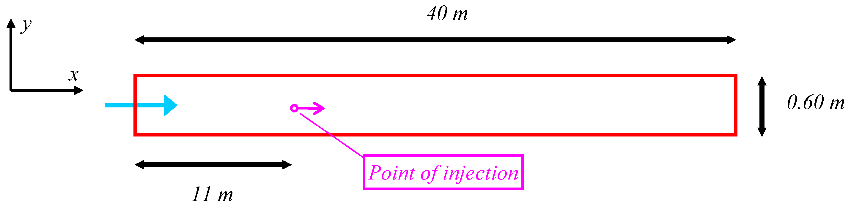
Figure 2.
Schematic plan view of the solute transport case study: (a) a contact tank that features meandering flow as indicated by vectors; (b) cross-sectional view of the channel inlet and Compartment 1 (dimensions in mm).
Figure 2.
Schematic plan view of the solute transport case study: (a) a contact tank that features meandering flow as indicated by vectors; (b) cross-sectional view of the channel inlet and Compartment 1 (dimensions in mm).

Figure 3.
Residence time distribution curves predicted for different sampling points at the tracer sampling points at: (a) z/Ht = 0.5 in Compartment 3; (b) z/Ht = 0.5 in Compartment 5; (c) z/Ht = 0.5 in Compartment 7; and (d) at the outlet.
Figure 3.
Residence time distribution curves predicted for different sampling points at the tracer sampling points at: (a) z/Ht = 0.5 in Compartment 3; (b) z/Ht = 0.5 in Compartment 5; (c) z/Ht = 0.5 in Compartment 7; and (d) at the outlet.

Figure 4.
Dispersion index values predicted numerically and experimentally for the contact tank tracer sampling points at (a) z/Ht = 0.05 in; (b) z/Ht = 0.5; (c) z/Ht = 0.95.
Figure 4.
Dispersion index values predicted numerically and experimentally for the contact tank tracer sampling points at (a) z/Ht = 0.05 in; (b) z/Ht = 0.5; (c) z/Ht = 0.95.
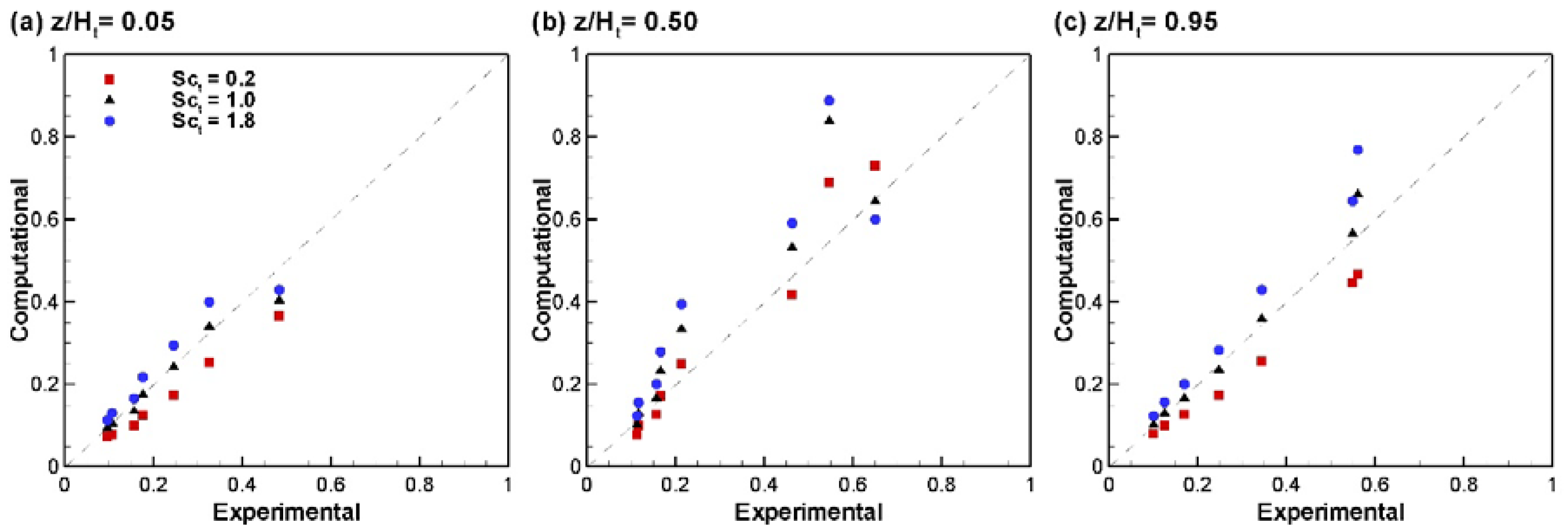
Figure 5.
Comparison of numerical results of carrier velocity, sediment concentration and total kinetic energy (TKE) for tests by [93]: (a) PS03; (b) PS08; (c) PS13; and a test by [48]: (d) NS1. Adapted from [43]. The circles represent the experimental data, and the solid line represents the numerical result.

Figure 6.
Comparison of numerical results (open symbols) with experiments (filled symbols) contributed by different authors for Sct in a particle-laden, open-channel flow. Adapted from [45] and modified for the present contribution. PTFM/CTFM and PTFMND/CTFMND are dilute and non-dilute models, respectively. S13, S14 and S16 refer to the test cases of [96]. The solid line indicates values obtained from the van Rijn (1984) formula.


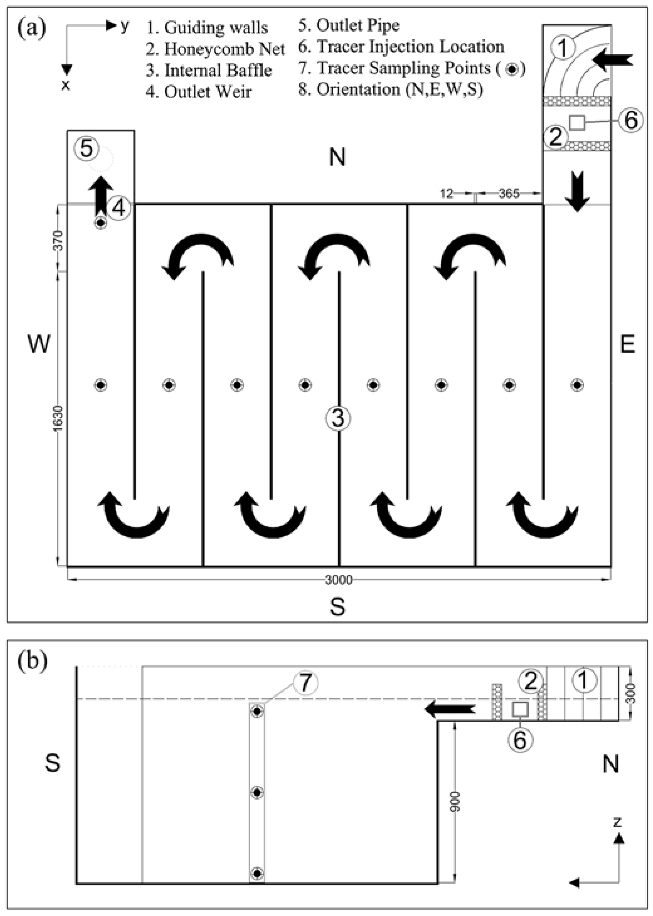
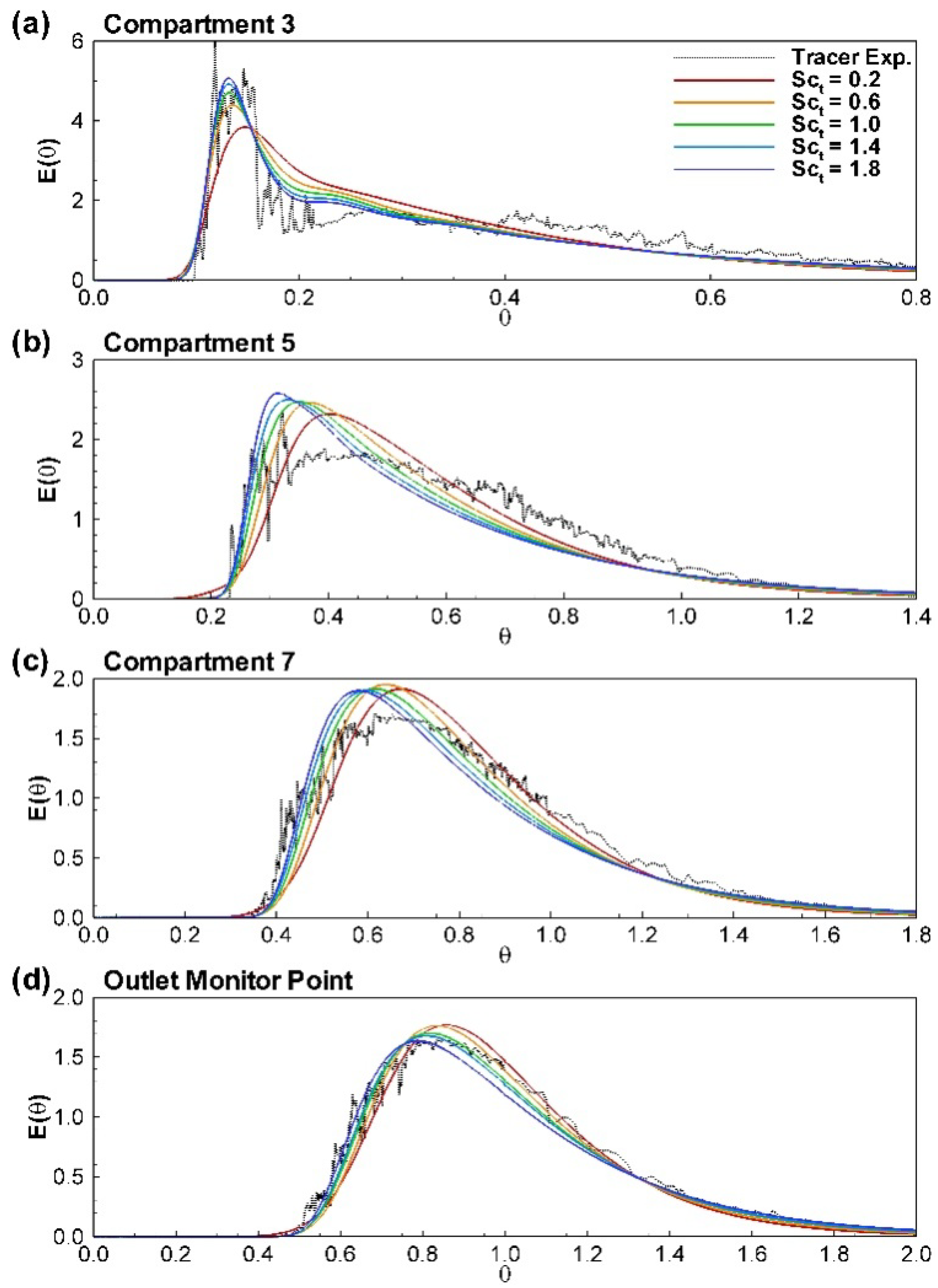
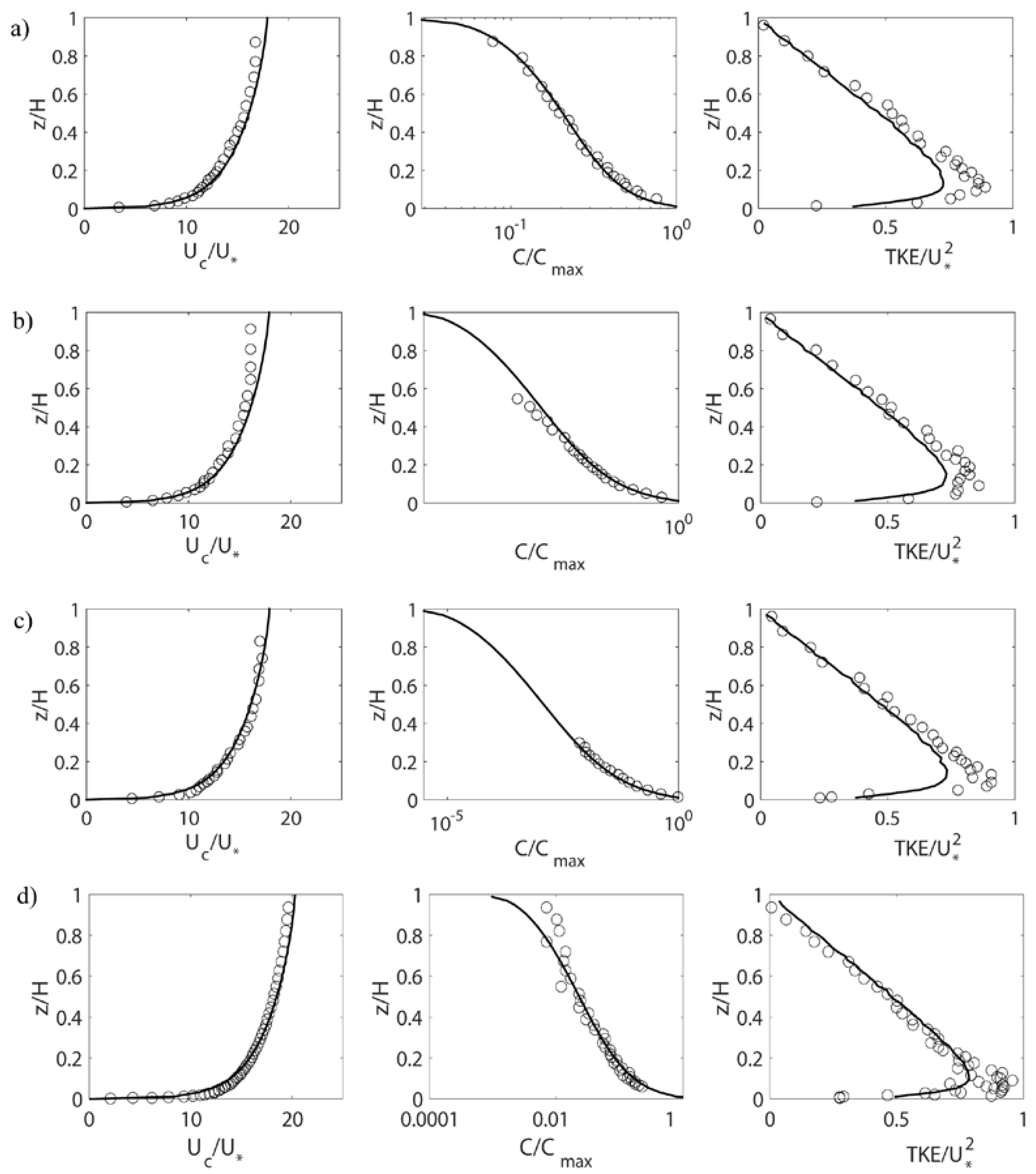
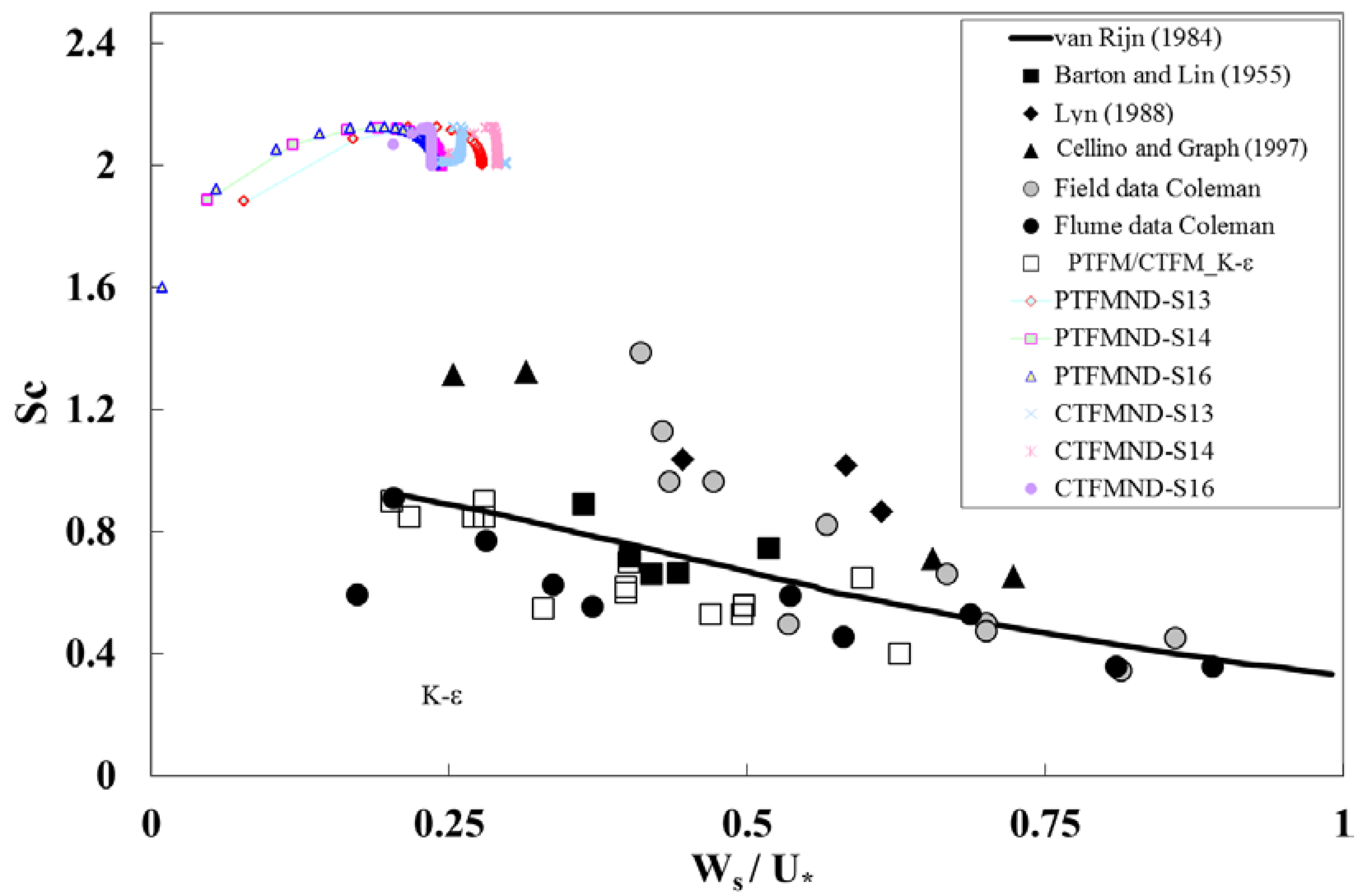
Table 1.
Values of the Schmidt number for different substances in air and water.
| Substance | Formula | Schmidt Number Sc for T = 25 °C | |
|---|---|---|---|
| Air | Water | ||
| Methane | CH4 | 0.99 | 570 |
| Oxygen | O2 | 0.84 | 441 |
| Nitrogen | N2 | --- | 240 |
| Carbon dioxide | CO2 | 1.14 | 410 |
| Ammonia | NH3 | 0.57 | 360 |
| Ethanol | C2H6O | 1.50 | 540 |
| Methanol | CH3OH | 1.14 | 540 |
| Cyclohexane | C6H12 | --- | 985 |
Table 2.
Values of the turbulent Schmidt number from water systems literature. Exp, experimental; Num, numerical.
Table 2.
Values of the turbulent Schmidt number from water systems literature. Exp, experimental; Num, numerical.
| Reference | Environmental Flow | Comments |
|---|---|---|
| Arnold et al. [22] | Flow and tracer transport in open channels | Exp − Sct = 0.5–0.9 |
| Djordjevic [23] | Flow and tracer transport in open channels | Exp/Num − Sct = 1 |
| Lin and Shiono [24] | Flow and tracer transport in open channels | Exp/Num − Sct = 0.72 |
| Simões and Wang [25] | Flow and tracer transport in open channels | Exp/Num − Sct = 0.5 (horizontal), 1 (vertical) |
| Gualtieri [30] | Flow and tracer transport in a contact tank | Exp/Num − Sct = 1 |
| Rauen et al. [33] | Flow and tracer transport in a contact tank | Exp/Num − Sct = 1 |
| Kim et al. [31] | Flow and tracer transport in a contact tank | Exp/Num − Sct = 0.3 |
| Zhang et al. [34,35,36] | Flow and tracer transport in a contact tank | Exp/Num − Sct = 0.7 |
| Angeloudis et al. [26,27,28,29] | Flow and tracer transport in a contact tank | Exp/Num − Sct = 0.7 |
| Martínez-Solano et al. [32] | Flow and tracer transport in a water tank | Exp/Num − Sct = 0.7 |
| Oliver et al. [37] | Inclined negatively buoyant discharges | Exp/Num − Sct = 0.6 |
| Graf and Cellino [41] | Sediment-laden open channel flows | Exp − Sct > 1 (no bedforms), Sct < 1 (bedforms) |
| Hsu and Liu [42] | Sediment-laden open channel flows | Exp/Num − Sct = 0.7 |
| Amoudry et al. [39] | Sediment-laden open channel flows | Exp/Num − Sct = 0.7 (bed), Sct = 0.52 (surface) |
| Muste et al. [47,48] | Sediment-laden open channel flows | Exp − Sct = 1. 4–2.11 (sand), Sct = 0.22–0.52 (nylon) |
| Toorman [52] | Sediment-laden open channel flows | Exp/Num − Sct = 0.5–0.8 |
| Bombardelli and Jha [40] | Sediment-laden open channel flows | Exp/Num − Sct = 0.56–0.7 (dilute mixtures) |
| Jha and Bombardelli [44,45,46] | Sediment-laden open channel flows | Exp/Num − Sct = 0.4–0.9 (k-ε model) |
| Jha [43] | Sediment-laden open channel flows | Exp/Num − Sct = 0.2–1.3 |
| Absi [38] | Sediment-laden open channel flows | Exp/Num − Sct = Sct (z) |
| Huang et al. [49] | Density stratified turbulence | Exp/Num − Sct = 1.3 |
| Huq and Stewart [50] | Density stratified turbulence | Exp − Sct = Sct (Ri, T*) |
| Walker et al. [51] | T-junction mixing experiments | Exp/Num − Sct = 0.1–0.2 |
Table 3.
Values of the turbulent Schmidt number from atmospheric systems literature.
| Reference | Environmental Flow | Comments |
|---|---|---|
| Koeltzsch [66] | Tracer transport in a boundary layer | Exp − Sct = 0.3–1, Sct = Sct (BL height) |
| Flesch et al. [63] | Contaminant emission from soil | Exp − Sct = 0.6 |
| Wilson [69] | Concentration measurements above a wheat crop | Exp − Sct = 0.68 and 0.78 |
| Tominaga and Stathopoulos [67] | Review paper | Exp/Num − Sct = 0.2–1.3 |
| Riddle et al. [68] | Pollutant dispersion in the built environment | Exp/Num − Sct = 0.3 and 0.7 |
| Di Sabatino and Buccolieri [61] | Pollutant dispersion in the built environment | Exp/Num − Sct = 0.4 and 0.7 |
| Blocken et al. [58] | Pollutant dispersion in the built environment | Exp/Num − Sct = 0.3–1 |
| Chavez et al. [59] | Pollutant dispersion in the built environment | Exp/Num − Sct = 0.1–0.7 |
| Mokhtarzadeh-Dehghan et al. [54] | Pollutant dispersion in the built environment | Exp/Num − Sct = 0.4–2.5 as f(Ri*) |
| Ebrahimi and Jahangirian [62] | Pollutant dispersion in the built environment | Exp/Num − Sct = 0.7 |
| Chen et al. [60] | Pollutant dispersion in the built environment | Exp/Num − Sct = 1.0 and corrected from wind tunnel data |
| Hassan et al. [65] | Supersonic crossflow | Exp/Num − Sct = 1.0 and adaptive Sct |
| Galeazzo et al. [64] | Jet in crossflow | Exp/Num − Sct = 0.3–0.9 |
| Goldberg et al. [70] | Different type of air flows | Exp/Num − Sct variable |
| Ross [71] | Flow over forested hills | Exp/Num − Sct = Sct (z) |
| Shi et al. [72] | Density stratified jets | Exp/Num − Sct = Sct (velocity and density gradient) |
Table 4.
Numerical simulations carried out.
| Run | Sct | Dt-y (m2/s) | Reference |
|---|---|---|---|
| Exp. | --- | 1.41 × 10⁻⁴ | Lau and Krishnappan [74] |
| 1 | 0.8 | 2.10 × 10⁻⁴ | Present study |
| 2 | 0.9 | 1.95 × 10⁻⁴ | Present study |
| 3 | 1.0 | 1.88 × 10⁻⁴ | Gualtieri [73] |
| 4 | 1.2 | 1.51 × 10⁻⁴ | Present study |
| 5 | 1.3 | 1.42 × 10⁻⁴ | Present study |
Table 5.
Hydraulic efficiency indicators values drawn from numerical model predictions where Sct values are in the range of 0.2–1.8 and the tracer experiment study results, respectively.
Table 5.
Hydraulic efficiency indicators values drawn from numerical model predictions where Sct values are in the range of 0.2–1.8 and the tracer experiment study results, respectively.
| Numerical Model Sct | Outlet Hydraulic Efficiency Indicators | |||||
|---|---|---|---|---|---|---|
| tp/T | t10/T | t90/T | tg/T | Μο | σ2 | |
| 0.2 | 0.904 | 0.702 | 1.345 | 0.991 | 1.933 | 0.074 |
| 0.4 | 0.843 | 0.700 | 1.356 | 0.994 | 1.938 | 0.077 |
| 0.6 | 0.834 | 0.695 | 1.374 | 0.998 | 1.976 | 0.082 |
| 0.8 | 0.825 | 0.690 | 1.391 | 1.001 | 2.015 | 0.088 |
| 1.0 | 0.817 | 0.685 | 1.407 | 1.004 | 2.052 | 0.093 |
| 1.2 | 0.809 | 0.681 | 1.421 | 1.006 | 2.087 | 0.099 |
| 1.4 | 0.802 | 0.677 | 1.435 | 1.009 | 2.120 | 0.104 |
| 1.6 | 0.794 | 0.674 | 1.448 | 1.011 | 2.150 | 0.108 |
| 1.8 | 0.788 | 0.671 | 1.460 | 1.013 | 2.177 | 0.113 |
| Exp. | 0.833 | 0.695 | 1.418 | 1.005 | 2.113 | 0.097 |
tp = peak concentration time, t10 = time until the passage of 10% tracer mass, t90 = time until passage of 90% tracer mass, tg = time corresponding to centroid of the Residence Time Distribution (RTD), Mo = Morrill index (= t90/t10), σ2 = dispersion index.
Table 6.
List of datasets used in this and other studies developed by the authors (expanded from [44]).
Table 6.
List of datasets used in this and other studies developed by the authors (expanded from [44]).
| Authors | Technique for Velocity Measurements | Variables Observed * |
|---|---|---|
| Lyn [92] | Laser-Doppler anemometry | Vmix, C |
| Muste and Patel [47] | Discriminator laser-Doppler velocimetry | Vc, Vd, T |
| Nezu and Azuma [93] | Particle tracking velocimetry | Vc, Vd, C, T |
| Muste et al. [48] | Particle image velocimetry and particle tracking velocimetry | Vc, Vd, C, T |
* V = velocity profiles; mix: mixture; c = carrier phase; d = disperse phase; C = concentration profile; T = turbulence statistics.
© 2017 by the authors. Licensee MDPI, Basel, Switzerland. This article is an open access article distributed under the terms and conditions of the Creative Commons Attribution (CC BY) license (http://creativecommons.org/licenses/by/4.0/).
Share and Cite
MDPI and ACS Style
Gualtieri, C.; Angeloudis, A.; Bombardelli, F.; Jha, S.; Stoesser, T. On the Values for the Turbulent Schmidt Number in Environmental Flows. Fluids 2017, 2, 17. https://doi.org/10.3390/fluids2020017
AMA Style
Gualtieri C, Angeloudis A, Bombardelli F, Jha S, Stoesser T. On the Values for the Turbulent Schmidt Number in Environmental Flows. Fluids. 2017; 2(2):17. https://doi.org/10.3390/fluids2020017
Chicago/Turabian StyleGualtieri, Carlo, Athanasios Angeloudis, Fabian Bombardelli, Sanjeev Jha, and Thorsten Stoesser. 2017. "On the Values for the Turbulent Schmidt Number in Environmental Flows" Fluids 2, no. 2: 17. https://doi.org/10.3390/fluids2020017