
Comment on Tailleux, R. Neutrality versus Materiality: A Thermodynamic Theory of Neutral Surfaces. Fluids 2016, 1, 32

1
School of Mathematics and Statistics, University of New South Wales, Sydney, NSW 2052, Australia
2
Lamont-Doherty Earth Observatory, Columbia University, Palisades, NY 10964, USA
3
Geophysical Fluid Dynamics Laboratory, National Oceanic and Atmospheric Administration (NOAA), Princeton, NJ 08540, USA
*
Author to whom correspondence should be addressed.
Fluids 2017, 2(2), 19; https://doi.org/10.3390/fluids2020019
Submission received: 27 March 2017
/
Revised: 27 March 2017
/
Accepted: 20 April 2017
/
Published: 26 April 2017
(This article belongs to the Collection Geophysical Fluid Dynamics)
Abstract
:Tailleux has written about the concept of epineutral mixing and has attempted to justify it from an energetic viewpoint. However, Tailleux’s approach is incorrect because it ignores the unsteady nature of the density field during baroclinic motions, which in turn leads to incorrect conclusions. Tailleux also asserts that “adiabatic and isohaline parcel exchanges can only be meaningfully defined on material surfaces” that are functions of only Absolute Salinity and Conservative Temperature and are not separately a function of pressure. We disagree with this assertion because there is no physical reason why the ocean should care about a globally-defined function of Absolute Salinity and Conservative Temperature that we construct. Rather, in order to understand and justify the concept of epineutral mixing, we consider the known physical processes that occur at the in situ pressure of the mixing. The Tailleux paper begins with two incorrect equations that ignore the transience of the ocean. These errors echo throughout Tailleux, leading to sixteen conclusions, most of which we show are incorrect. (Comment on Tailleux, R. Neutrality Versus Materiality: A Thermodynamic Theory of Neutral Surfaces. Fluids 2016, 1, 32, doi:10.3390/fluids1040032.)
1. Overarching Comments on Tailleux
The direction of the mixing associated with stirring by mesoscale oceanic turbulence has been described as “isopycnal” since Iselin [1] The fully nonlinear equation of state of seawater was incorporated into the definition of “neutral surfaces” by McDougall [2,3]. A detailed justification of these “neutral surfaces”, or more precisely “neutral directions”, as being the direction of the mixing by mesoscale eddies had to wait until Section 7.2 of Griffies [4], Section 2 of McDougall and Jackett [5], and recently, Section 1a of McDougall et al. [6]. These authors invoked the ocean measurements of small-scale mixing that have accumulated since the 1980s. These measurements show that interior ocean small-scale mixing is very small relative to lateral mixing, and this small-scale mixing is not obviously related to the strength of mesoscale eddy-induced lateral stirring and mixing. Making use of a reductio ad absurdum argument, McDougall et al. [6] explained why ocean mixing measurements can be interpreted as empirical justification for taking the stirring and mixing from mesoscale eddies to be directed along the locally-referenced potential density surface; i.e., along the neutral direction. This issue is fundamental to how we conceptualize mesoscale eddy stirring and the associated tracer mixing, and furthermore how we parameterize tracer mixing in numerical models that are too coarse to resolve mesoscale eddies.
Tailleux [7] was not convinced by the empirically based reasoning of McDougall et al. [6]. Instead, Tailleux attempted to find arguments based on first principles. Although it was a noble attempt and a good question to ask, we here show that many of the arguments in Tailleux [7] are incorrect or unfounded. Although we consider almost all of Tailleux [7] to be incorrect, the question that paper asked inspired us in McDougall et al. [8] to further motivate, more thoroughly explain, and to update the arguments presented in McDougall et al. [6].
In this comment, we discuss Tailleux [7] in detail to highlight the parts that are incorrect, of which the most important ones are highlighted in this introduction.
- Tailleux [7] misunderstands or misinterprets the justification, as published by Griffies [4], McDougall and Jackett [5], and McDougall et al. [6], that the energetic lateral mixing of mesoscale eddies occurs in the locally-referenced potential density surface. For example, Tailleux [7] quotes McDougall et al. [6] as implying that the individual fluid motions in mesoscale eddies move across the locally-referenced potential density surface. In contrast, McDougall et al. [6] discuss these motions only as part of a reductio ad absurdum proof. That is, McDougall et al. [6] specifically conclude, based on ocean measurements, that this dianeutral motion is NOT what occurs in the ocean. Moreover, inexplicably, Tailleux [7] asserts that while individual motions are diabatic, their average is adiabatic. This is incorrect. Rather, if individual motions are diabatic, then the average of many such motions exhibits dianeutral diffusion.
- Tailleux [7] states that, (1) in order for an adiabatic and isohaline displacement of a fluid parcel over a distance to be neutral, then (his Equation (1), where is the normal vector to the neutral tangent plane); and (2) then goes on to state that (his Equation (7)) is the buoyant force experienced by fluid parcels after such an adiabatic and isohaline displacement. Both of these statements are generally incorrect. Indeed, we consider these two incorrect equations to be at the core of the errors that permeate Tailleux [7]. The reason these equations are generally incorrect is that they ignore the unsteady nature of baroclinic motion. These two equations are only correct if the ocean hydrography is in a steady state. This is the case for a hydrographic atlas, but is it not appropriate for discussions of the underlying physics and energetics of epineutral mixing. For such discussions, it is crucial to properly account for unsteadiness of the flow during baroclinic instability and the associated release of available potential energy.
- Tailleux [7] asserts that “adiabatic and isohaline parcel exchanges can only be meaningfully defined on material surfaces of the form ”. We disagree with this statement. There is no fundamental reason that the ocean should oblige in this regard. Rather, we oceanographers should examine ocean mixing in terms of known physical processes that occur at the in situ pressure of the mixing. (Tailleux [7] uses potential temperature and an undefined type of salinity. Since Absolute Salinity and Conservative Temperature are the recommended salinity and temperature variables for use in oceanographic publications (see Valladares et al. [9] and Intergovernmental Oceanographic Commission (IOC) et al. [10]), we have adopted these variables in this paper).
2. Comments on Section 1 of Tailleux
Equation (1) of Tailleux [7], namely does not generally describe the displacement of an adiabatic and isohaline motion as claimed. Rather, such an adiabatic and isohaline displacement requires that the velocity obeys
which is equivalent to the statement that the locally-referenced potential density does not change for a small neutral displacement, that is, . Hence, the correct version of Tailleux’s [7] Equation (1) is
By contrast, throughout Tailleux [7] the neutral relationship is written as Equation (1) of that paper, which is .
This same neglect of transience occurs in Equations (4), (6), and (7) of Tailleux [7]. In the discussion of Equation (7) of that paper, Tailleux [7] incorrectly states that “the buoyancy of fluid parcels experiencing adiabatic and isohaline lateral displacements is—without approximation—given by” . The key error Tailleux makes here is to assume that the buoyancy force is equal to , thus neglecting the ocean’s transience. Tailleux’s Equation (7) is not “the buoyancy of fluid parcels experiencing adiabatic and isohaline lateral displacements” as claimed, instead, it is the temporal rate of change of buoyancy at a fixed point in space for an adiabatic and isohaline displacement.
Apparently due to this error, Tailleux [7] goes on to state that the individual parcel displacements are likely not adiabatic and isohaline. Furthermore, and without explanation, Tailleux [7] then assumes that the average of many such diabatic displacements may well be adiabatic. If indeed the individual displacements were diabatic (which we dispute), then it would be very unlikely that the mean dianeutral motion would be zero. However, even if this were the case, the integrated effect of many such diabatic displacements will have the character of dianeutral diffusion (to see this, simply perform the averaging in density coordinates), and this is the opposite of the conclusion drawn by Tailleux [7].
Throughout Tailleux [7] the author describes the traditional justification of McDougall [2] and McDougall et al. [6] as being based on “the momentum equation” and hence is a “dynamical concept”. This statement is not correct. The explanation of the neutral concept and of the locally-referenced potential density surface is not based on the momentum equations, nor is it based on energetic considerations, nor is it a dynamical concept. Rather, the arguments of McDougall et al. [6] are a direct and inevitable consequence of the absence of vertical static instabilities except during active turbulence inside individual small-scale mixing events of the Kelvin Helmholtz variety.
In McDougall et al. [8] we have shown that any small-scale turbulence must be treated as an extra dianeutral diffusivity and specifically not as mixing in a direction other than the locally-referenced potential density surface. Tailleux [7] belabours the difference between a “dynamical” and a “thermodynamical” constraint. It is unclear what Tailleux [7] means by these statements; especially so as both Equations (4) and (6) of Tailleux [7], which are central to the discussion, are incorrect since they both neglect the ocean’s transience.
3. Comments on Section 2 of Tailleux
Tailleux [7] misinterprets the arguments we presented in Figure 1 of McDougall et al. [6]. The key focus of this figure is to point out that mixing arising from baroclinic instability does NOT occur by the two paths depicted in this figure. In contrast, Tailleux [7] has adopted as realistic the advection of Figure 1 through the locally-referenced potential density surface, followed by the subsequent dianeutral mixing. This perspective is exactly what McDougall et al. [6] argue does not occur in the ocean. The two-step process of their Figure 1 was part of McDougall et al.’s reductio ad absurdum proof. That is, one assumes something and then shows that this assumption cannot be correct because it leads to a contradiction: the assumption is “absurd”. Inexplicably, the first step of McDougall et al.’s Figure 1, namely the adiabatic and isohaline displacement through the locally referenced potential density surface, is adopted by Tailleux [7] as being part of the McDougall et al. [6] argument. However, the opposite is the case. Namely, this is exactly the step that we argued does not occur in the ocean! This fundamental misinterpretation of McDougall et al.’s physical argument dominates Section 2 of Tailleux [7]. Indeed, it colours the whole of Tailleux [7].
Tailleux [7] confuses the issue of transience with the non-zero buoyant force experienced by a fluid parcel that is displaced through a locally-referenced potential density surface. For example, near the bottom of page 6 of Tailleux [7] one reads “a non-zero buoyancy force does not imply diapycnal mixing…just transience, as attested by Equation (7)”. This statement is incorrect. If a fluid parcel were to be displaced through the locally-referenced potential density surface, and then released and allowed to interact with its surroundings, then it would indeed mix turbulently with the surrounding ocean. This process is called plume dynamics in the geophysical fluid dynamics literature [11]. This was the point of the McDougall et al. [6] argument, and this argument holds whether or not the flow is steady or unsteady.
The key word in the preceding paragraph is “through” as opposed to “normal to”. The buoyant force felt by the fluid parcel is not Tailleux’s Equation (7), but rather it is only due to motion of the parcel through the density surface. For more discussion on the flow through a surface (including moving surfaces) we refer to Griffies [4] (pp. 138–141) and Groeskamp et al. [12] (Figure 3). This incorrect expression for the buoyant restoring force in Tailleux [7] has led to many other incorrect aspects of Tailleux [7].
Tailleux [7] discusses (in Section 2.3.2) the energetic implications of a general displacement and finds that energy can be released by displacements in the wedge of instability. This is a standard result of baroclinic instability theory. Tailleux [7] also finds that if the fluid displacement is directed in the neutral tangent plane ( in the terminology of Tailleux [7]) then no energy will be released or required. However, because Tailleux [7] incorrectly associates the constraint with displacements that incur no buoyant restoring force, Tailleux [7] also incorrectly associates with epineutral displacements and epineutral mixing. This association is incorrect because of transience. Neutral motion occurs when the buoyant restoring force on a parcel is zero, not when the instantaneous velocity vector has no component normal to the neutral tangent plane, that is, when . Transience makes these things unequal. The reader is referred to Section 3 of McDougall et al. [8] for a detailed explanation of the difference.
If Section 2.3.2 of Tailleux’s paper were correct, then epineutral mixing would require that the fluid displacements satisfy , in which case fluid motion in the wedge of instability (which has ) would not be neutral and so would exhibit substantial dianeutral turbulent mixing. We know this to be incorrect as baroclinic instability can occur in the absence of any dianeutral mixing. Indeed, baroclinic instability is routinely taught from the perspective of immiscible layers of ideal fluid in which no fluid is transferred between layers.
Tailleux [7] considers (in Section 2.3.4) the mixing of a variable that is a function of only Absolute Salinity and Conservative Temperature, . The mixing is performed with epineutral diffusion (normal to ) as well as dianeutral diffusion, presumably in an eddy-less ocean model context where the hydrographic data is steady (no transience). Tailleux [7] shows that the mixing of normal to its iso-surfaces occurs with an extra diffusivity equal to essentially the epineutral diffusivity times the square of the slope difference between the neutral tangent plane and the surface. This result is expected and is analogous to the so-called Veronis effect for horizontal mixing (Veronis [13]). However, then Tailleux [7] incorrectly asserts that the globally defined variable must have some significance to the issue of local mixing processes and that we should attempt to minimize the extra unintended mixing across the iso-surfaces of .
There is no reason for the ocean to pay special attention to an arbitrary variable of our construction. For example, consider the specific case of being equal to the Conservative Temperature itself. In this case, epineutral mixing will mix along its epineutral gradient, resulting in a substantial effective diffusivity across surfaces. This behaviour is expected and we should not attempt to minimize this diffusion across surfaces. Since this particular example of is unphysical, we ask how are we to construct a physical basis for a different variable that is a global function only of Absolute Salinity and Conservative Temperature (and is independent of pressure), which has the property that baroclinic motions mix along its iso-surfaces? This aim is not realizable in the ocean.
Rather than attempting to impose a human-conceived, globally-defined variable as a new anthropogenic constraint on ocean mixing dynamics, we instead look to ocean physics for inspiration regarding ocean mixing. In particular, the pressure at which mixing occurs is central to how we understand ocean mixing. In McDougall et al. [8] we consider the physical processes that occur in baroclinic instability, and we emphasize that any small-scale mixing that occurs during baroclinic instability will occur by the Kelvin Helmholtz instability mechanism, a mechanism that occurs while the vertical density gradient is stable. The relevant function to be considered when local mixing processes are considered is the locally-defined potential density, . The reference pressure of this potential density variable is the local in situ pressure at which the mixing is occurring, and is clearly not a globally-defined variable.
McDougall et al. [8] explore the consequences of lateral mixing oriented in a surface other than the locally-defined potential density surface. We show there that the extra fictitious dianeutral diffusivity is different for each passive tracer and that these fictitious diffusivities are not only unequal, but are as often negative as positive. This property of the fictitious diffusivities is a fundamental deficiency of non-neutral mixing since turbulent mixing processes mix passive “potential” properties with equal and positive turbulent diffusivities.
4. Comments on Section 3 of Tailleux
Section 3.1 of Tailleux [7] continues to assume that lateral mixing is oriented according to a globally defined surface, and continues to assert that the buoyant force in the neutral density literature had been assumed to be , again misunderstanding the role of transience in baroclinic instability.
The caption to Tailleux’s Figure 3 is incorrect. This caption reads “Fluid parcel trajectories, depicted as the red arrows, must lie at the intersection of surfaces of constant potential temperature and salinity for adiabatic and isohaline displacements caused by stirring.” However, if lateral displacements occurred along the line of intersection of Conservative Temperature and Absolute Salinity then there would be no epineutral mixing of heat and salt. Rather, the lateral displacements that lead to epineutral mixing lie in the locally-referenced potential density surface but are not along the line of intersection of Conservative Temperature and Absolute Salinity.
Section 3.2 of Tailleux [7] discusses the energetic implications of mixing in various directions, as summarized in Figure 4 of that paper. This figure depicts the exchange of two fluid parcels along a surface, with the angle of the exchange being between the horizontal direction and the slope of the neutral tangent plane, so this parcel exchange releases potential energy. Figure 4a of Tailleux [7] is very similar to Figure 1 of McDougall et al. [6], but the conclusions drawn are diametrically opposite. In McDougall et al. [6] (and in McDougall et al. [8]) we argue that while fluid parcels may well move in the wedge of instability when undergoing baroclinic instability, the fluid parcels do not move through the locally-referenced potential density surface. The distinction is again because of transience. A neutral parcel velocity satisfies during baroclinic instability (that is, there is no change in locally-referenced potential density following the flow during neutral motion). Furthermore, the velocity involved in this motion, , does not satisfy ; that is, Tailleux’s Equation (1), , is not satisfied.
In McDougall et al. [6] we argued that fluid parcels are not transported through locally-referenced potential density surfaces in the manner depicted in Tailleux’s Figure 4a. If this dianeutral motion were to occur, strong small-scale turbulence would be measured along with strong baroclinic eddy motions in the ocean. In McDougall et al. [8] we have generalized this discussion to allow for the possibility that small-scale turbulent mixing might occur as a direct result of baroclinic eddy motions. We have shown that such small-scale mixing must be represented as isotropic down-gradient diffusion and not as mixing along a non-neutral direction. Simply put, the vertical static instability associated with Tailleux’s Figure 4a is not observed in the ocean, and the Kelvin-Helmholtz instability would grow well before the fluid parcels found themselves to be unstably stratified as in Figure 4a.
We refer to the mixing achieved by active small-scale turbulence as being isotropic, although the isotropy of this small-scale mixing has rarely been confirmed by observation. There is some indication that when the mixing is very active, the turbulent diffusivity of the mixing may be regarded as being isotropic [14], while when the mixing is weak, it mixes preferentially along the density surfaces and is suppressed in the dianeutral direction [15]. We will continue to refer to the small-scale turbulent as being isotropic, to emphasise that it does not mix simply in the vertical or dianeutral direction.
Tailleux [7] states that Figure 4a of that paper cannot apply unless there are epineutral gradients of Conservative Temperature and Absolute Salinity, which seems strange (since baroclinic instability can occur in a large stratified freshwater lake), until one realizes that the whole of Figure 4 is predicated on mixing along a surface. The situation of Figure 4a thus precludes that could be the locally-referenced potential density surface in an ocean with no salinity gradients.
In discussing the three panels of Figure 4, Tailleux [7] notes that in the case of panel (a) the parcels are further apart after the parcels are released and have found their level of neutral buoyancy, than they were after their initial lateral displacement. Tailleux calls this case “super-dispersive”. While this behaviour may appear to be the case in Figure 4 with its traditional vertical exaggeration, the extra distance is only proportional to the ratio of the square of the slope of the locally-referenced potential density surface, that is, it is a negligible effect. For example, with a neutral tangent plane slope of , a lateral diffusivity would possibly be increased by 50 parts in a million () due to this effect, taking a lateral diffusivity from say to ; a totally trivial increase.
In Section 3.3, Tailleux [7] proves (his Equation (32)) that when mixing is confined to be along the locally-referenced potential density surface, the energy cost of the parcel exchange is zero. However, the energy cost is further studied in Tailleux’s Appendix B, where again there is confusion between the optimal direction in which parcels move in baroclinic instability, called the “optimal stirring direction” in Figure B2 of Tailleux [7], and the occurrence of small-scale dianeutral mixing. Contrary to the paragraph between Equations (79) and (80) of Appendix B of Tailleux [7], the movement of fluid parcels in the wedge of instability does not directly result in small-scale dianeutral mixing. Rather, fluid parcels can move in the wedge of instability where while the flow is 100% adiabatic and isohaline. The key to understanding this property is (a) to account for the unsteadiness of the flow, and (b) to realize that if small-scale turbulence is initiated, it will occur via the Kelvin Helmholtz instability process while the vertical stratification is stably stratified, and so will transport all passive “potential” variables in a down-gradient manner with the same turbulent diffusivity. By contrast, mixing laterally in a non-neutral direction involves unequal and even negative fictitious dianeutral diffusivities (see McDougall et al. [8]).
5. Comments on Section 6 of Tailleux
The Summary and Conclusions section of Tailleux [7] (Section 6 of that paper) consists of sixteen bulleted paragraphs. We here comment on many of these paragraphs, showing that most of them are incorrect.
5.1. Tailleux’s First Conclusion
Tailleux’s [7] first bullet point of the Summary and Conclusions section says that “…the physical processes for lateral dispersion in the ocean must in general have a non-zero buoyancy…”. This statement is incorrect and seems to be based on Tailleux’s association of with the buoyant force acting on a fluid parcel. As explained above, is not proportional to the buoyant restoring force in unsteady situations such as during baroclinic instability. The movement of a fluid parcel in the wedge of instability guarantees that . However, since the surface itself moves, there is no need for a fluid parcel to move through the locally-referenced potential density surface as it moves in the wedge of instability. That is, even though , there need be no dianeutral motion and no buoyant force on the fluid parcel. When averaging over many such stirring events, each of which is neutral, the average is also neutral.
The first bullet point also says “The concept of epineutral dispersion, therefore, only makes sense if viewed as the aggregate result of many individual non-neutral (i.e., having non-zero buoyancy) stirring events.” This is physically impossible, and it is not clear what led Tailleux [7] to this conclusion. If indeed the individual mixing events involved non-neutral excursions, then averaging over many such events may (possibly, but very unlikely) result in no mean flow through the locally-referenced potential density surface. However, such a collection of non-neutral parcel displacements would certainly result in non-zero diffusion through this locally-referenced potential density surface.
5.2. Tailleux’s Second Conclusion
The second bullet point of Tailleux’s [7] conclusion section begins with “It is not true that neutral trajectories obtained as solutions of the neutral tangent plane Equation (1) can describe actual trajectories, contrary to what is usually assumed, because such trajectories implicitly require the existence of non-material sources of heat and salt.” This statement is incorrect, as are the corresponding last two sentences of Section 2.3.3 of Tailleux [7]. That is, it is incorrect to state that neutral trajectories are usually assumed to be the trajectories of fluid parcels. The literature on neutral trajectories quite clearly does not take them to be the finite amplitude trajectories of material fluid parcels, and it is inexplicable how Tailleux [7] could misunderstand and misrepresent this fundamental aspect of the several papers on neutral trajectories, including the several papers concerned with the path-dependence of neutral trajectories. For example, the following papers, McDougall [2,3,16,17], McDougall and Jackett [5,18,19] and Klocker and McDougall [20,21] all describe neutral trajectories as the integration of the neutral relation defined at a point in space-time, and none of these papers confuse a neutral trajectory with a fluid parcel trajectory.
The reason that a neutral trajectory is not a fluid parcel trajectory is that along the neutral trajectory there are compensating changes in Absolute Salinity and Conservative Temperature, and these changes occur as a result of non-material mixing processes. In this second bullet point, and in our discussion of it here, the hydrographic data used to evaluate the neutral tangent plane is taken to be the result of substantial averaging, such as when the data being used is a smoothed hydrographic atlas, or is taken from a coarse-resolution, non-eddy-resolving ocean model.
The second sentence of the second bullet point reads “It is also not true that neutral tangent planes represent surfaces along which fluid parcels can be exchanged without experiencing (restoring or otherwise) buoyancy forces.” This statement is also incorrect. The neutral tangent plane is indeed such a surface, and it is explicitly defined to have exactly this property. The neutral tangent plane is defined for infinitesimally small lateral displacements and it is well-defined. Being a plane in space, it can only be exactly neutral as the limit of small amplitude displacements is taken. Finite amplitude neutral displacements that are both adiabatic and isohaline do deviate vertically from neutral trajectories, and this behaviour is the physics underlying the thermobaric dianeutral advection that has been studied in many papers in the literature (for example, McDougall [3,16], and Klocker and McDougall [20]).
The last two sentences of Tailleux’s second bullet point discusses finite amplitude lateral displacements and their thermobaric dianeutral motion as though this were an issue which questions the use of locally-referenced potential density surfaces. In fact, there is no such issue. Locally-referenced potential density surfaces are only neutral at the point of osculation with the neutral trajectories that pass through the point concerned. Moreover, the dianeutral advection caused by finite amplitude displacements does not question the concept and use of locally-referenced potential density surfaces. Rather, these finite amplitude dianeutral motions are an extra dianeutral advection process that occurs in the ocean, and this thermobaric advection process has been studied in several papers (e.g., McDougall [3,16], Iudicone et al. [22], Klocker and McDougall [20], and Groeskamp et al. [23]). Moreover, these processes are advective in nature, not diffusive. So, these aspects of epineutral mixing are very well known, and they are not spurious dianeutral mixing processes, but rather they are genuine dianeutral advection processes. The finite amplitude motion of adiabatic and isohaline displacements is studied in the appendix to this paper. This confirms that these neutral trajectories approach the locally-referenced potential density surface quadratically with the lateral displacement.
Moreover, if one insists on mixing in a globally-defined surface, then one obtains an approximate form of the cabbeling dianeutral advection, but, as first pointed out by Iudicone et al. [22], one does not obtain the thermobaric dianeutral advection (see also Appendix A.27 of IOC et al. [10]). Tailleux [7] prefers to imagine that the ocean mixes along a surface, but why would this be the case when in doing so the ocean would automatically delete a real physical process, thermobaricity, that occurs in the ocean?
Also, since is a function whose definition we choose, how would we choose the local slope of such a surface, compared with the slope of the neutral tangent plane? We have the freedom to increase this slope difference in one location and decrease it in another, and on what physical basis would we make this choice? Having made a subjective choice, we are obviously unable to communicate that choice to the ocean! We can think of no justification for any such choices for a globally-defined function. The approach we take is to define the properties of lateral mixing in accordance with the pressure at which the mixing is occurring and the physical ocean processes that are at work. Of course there are practical reasons why one might sometimes opt for the simplicity of a globally-defined function as an approximate description of a neutral density variable, but it is incorrect to argue that this functional form is justified by physical considerations.
5.3. Tailleux’s Third Conclusion
In the third bullet point of Section 6, Tailleux [7] reaches incorrect conclusions regarding the motion of a parcel in a transient ocean. This bullet point states that when a parcel moves in the wedge of instability (in which ), it has a non-zero buoyancy. This statement is incorrect. As explained above, a parcel feels a buoyant force only when it has a different density to the surrounding ocean, and when the ocean is unsteady this buoyant force is not simply proportional to .
Also, contrary to what Tailleux [7] claims in the first sentence of this third bullet point, the equation does not represent a neutral fluid parcel displacement in an unsteady ocean. Rather, neutral motion obeys , which can be written as our Equation (2) above. By contrast, throughout Tailleux [7] the neutral relationship is written as Equation (1) of that paper, which is . The constraint of does not come from “momentum considerations” as Tailleux [7] claims as the underlying motivation for Equation (1) of that paper; this equation being an incorrect version of neutrality in an unsteady ocean. Rather, is based on the physical processes at work during finite amplitude baroclinic instability as explained in McDougall et al. [6,8].
5.4. Tailleux’s Fourth Conclusion
The fourth bullet point of Section 6 of Tailleux [7] states incorrectly “Since the stirring events making up epineutral/isopycnal/lateral dispersion are usually non-neutral…”. This incorrect statement may arise from Tailleux’s incorrect definition of neutrality, namely Equation (1) of Tailleux [7], which is . Instead, the correct definition of neutrality is Equation (1) of the present paper. Because Tailleux [7] realized that Equation (1) of that paper is not satisfied during the unsteady baroclinic motion, the author then seems to have assumed that this means that the motion cannot be neutral. We have explained the error of this thinking in the previous paragraph. The rest of this fourth bullet point then postulates that the average motion over many non-neutral excursions may end up being neutral in the mean. This additional incorrect assertion is not needed since the individual displacements do not have to be non-neutral. However, putting this aside, the individual non-neutral excursions would result in diffusion through the locally-referenced potential density surface.
5.5. Tailleux’s Seventh Conclusion
The seventh bullet point of Section 6 of Tailleux [7] states that the unstable motion in the wedge of instability is associated with enhanced dispersion, meaning that in Figure 4a of Tailleux [7], the distance between the two parcels increases as they move vertically and find their levels of neutral buoyancy. However, the extra distance is increased over the purely horizontal distance between the parcels proportionally by only one half of the square of the slope of the neutral tangent plane; a truly negligible proportion, so this seventh bullet point is of trivial magnitude and is unimportant.
5.6. Tailleux’s Eighth Conclusion
The eighth bullet point in Section 6 is also based on Figure 4 of Tailleux [7]. This eighth bullet point insists that the ocean must mix laterally along a surface that is defined as a function only of Absolute Salinity and Conservative Temperature, . This insistence means that the surface can osculate with the neutral tangent plane only along a few lines in the ocean (this insight is gleaned from taking the special case of where it is a potential density surface referenced to a fixed reference pressure). However, in a salt-less ocean, surfaces (in this case these are surfaces of constant Conservative Temperature) can be neutral surfaces throughout the whole ocean, and mixing along the surface is the same as epineutral mixing. When the ocean does contain salinity gradients, this eighth bullet point incorrectly claims to have found “A new mechanism for enhanced lateral dispersion…”. This dispersion mechanism (as sketched in Figure 4a of Tailleux [7]) appears to be a new mixing mechanism, but it relies on the unphysical demand that the ocean mix along an anthropogenically chosen surface. This sketch is similar to Figure 1 of McDougall et al. [6], in which we made the point, in a reductio ad absurdum proof, that the dianeutral advection of Tailleux’s Figure 4a does not occur in the ocean. This dianeutral advection of a fluid parcel cannot occur because the Kelvin Helmholtz instability mechanism sets in well before fluid parcels find themselves unstably stratified as in Tailleux’s Figure 4a.
The first sentence of this eighth bullet point of Tailleux [7] alludes to the source of energy for the mixing mechanism of Figure 4a being the thermobaric term in the equation of state; see Equation (35) of Tailleux [7]. The mixing mechanism of Tailleux’s Figure 4a does not exist in the ocean. The appearance of the thermobaric coefficient in Equation (35) of Tailleux [7] reflects the fact that the parcels have been mixed in a non-neutral manner in Figure 4a. Furthermore, this mixing occurs in a direction whose slope with respect to the neutral tangent plane is proportional to the thermobaric coefficient times the difference between the in situ pressure and a reference pressure. Depending on the slope so obtained, sometimes this arbitrarily and unphysically-imposed mixing direction will lie in the wedge of instability and sometimes outside of it.
5.7. Tailleux’s Ninth Conclusion
The ninth bullet point in Section 6 of Tailleux [7] claims incorrectly that “the use of a neutral rotated diffusion tensor, as is the current practice in numerical ocean modelling, implies that the effective diapycnal diffusivity of all conceivable material density variables is potentially much larger than the value of the dianeutral diffusivity used in such tensors, raising the issue of whether the use of such tensors avoids or causes spurious diapycnal diffusion”.
This convoluted and incorrect conclusion of Tailleux [7] was reached as a result of the assertion in that paper that the lateral mixing occurs along surfaces of the globally defined variable rather than the lateral mixing being epineutral. We have shown above that the relevant surface in which the lateral mixing occurs is the surface of constant locally-referenced potential density, . The reference pressure of this potential density variable is the local in situ pressure at which the mixing occurs, and is clearly not a globally-defined field. Moreover, this part of Tailleux [7] (his Section 2.3.4) did not consider the implications of this non-neutral mixing along a surface on the spurious diffusivities of Absolute Salinity and Conservative Temperature separately. We have shown in McDougall et al. [8] that when lateral mixing is assumed to occur in a non-neutral direction, the extra fictitious dianeutral diffusivity is different for each passive tracer and these fictitious diffusivities are often negative; this is clearly undesirable.
5.8. Tailleux’s Eleventh Conclusion
The eleventh bullet point in Section 6 of Tailleux [7] suggests that “the realization that epineutral dispersion is actually made up of non-neutral stirring events …”. This suggestion is incorrect. It is again due to the incorrect definition of neutral motion in Tailleux [7] as arising from a velocity satisfying Equation (1) of that paper, namely, . Instead, neutral motion constrains the velocity vector according to our Equation (1) above. Consequently, Tailleux [7] did not in fact resolve “some longstanding apparent paradoxes and inconsistences …”, as claimed in this bullet point.
5.9. Tailleux’s Twelfth Conclusion
The twelfth bullet point in Section 6 claims that Tailleux [7] has clearly established “the relevance of energetics for categorizing the different possible dispersion regimes in the ocean …”. Rather, we have deduced the centrality of the neutral mixing process via considering the physical processes that occur in the growing and finite amplitude stages of baroclinically unstable motions, and specifically, we do not consider the changes in any type of energy during the turbulent motion. In McDougall et al. [8] we conjecture that it is unlikely that consideration of ocean energetics will be able to shed light on the direction of the strong mesoscale mixing processes. Moreover, contrary to what one reads in several places in Tailleux [7], the ideas underlying the neutral mixing direction are not based on consideration of the vertical momentum equation.
5.10. Tailleux’s Thirteenth Conclusion
The thirteenth bullet point in Section 6 claims that Tailleux [7] has dispelled “the widespread misconception, e.g., McDougall (1987), that the buoyancy forces involved in parcel exchanges in potential density surfaces are necessarily restoring”. It is hard to know exactly what Tailleux means by this remark. Certainly, the neutral mixing ideas do not preclude the existence of baroclinic instability, but it is important to note that baroclinic instability can and does occur without the need for any fluid parcel to be unstably stratified in the vertical. Also, if a local fluid parcel were moved through a locally-referenced potential density surface, then the vertical buoyant force is indeed always restoring, acting in the vertical direction opposite to the vertical dianeutral displacement that caused the buoyancy anomaly.
6. Conclusions
Tailleux [7] attempted to answer a relevant question: what is the direction of lateral mixing in the ocean and how can we derive it from first principles? This quest by Tailleux [7] seems to have been motivated by not being convinced by the empirical argument given in McDougall et al. [6], who argued that this direction is along the locally-referenced potential density surface. Unfortunately, Tailleux [7] made an incorrect assumption in an initial stage of the paper, and this incorrect assumption prevailed throughout the remainder of Tailleux [7], leading to many incorrect statements and conclusions. As a result, Tailleux [7] has the potential to cause unnecessary confusion on the topic of the direction of neutral mixing in the ocean. To avoid this confusion and provide corrections to the mistakes, we were prompted to write this response.
Acknowledgments
Although disagreeing with nearly every point made by Tailleux, the provocative nature of that paper motivated our attempt here to clarify misconceptions. Louise Bell of Bell Graphic Design (Tasmania) is thanked for preparing Figure 1. We gratefully acknowledge Australian Research Council support through grant FL150100090 (Trevor J. McDougall) and National Science Foundation support through grant OCE-1233832 (Sjoerd Groeskamp).
Conflicts of Interest
The authors declare no conflict of interest.
Appendix A
Neutral Trajectories at Finite Amplitude
The discussion of neutral trajectories in McDougall et al. [6] considered an infinitesimally small displacement of a seawater parcel in an adiabatic and isohaline manner. In this appendix, we extend that discussion to consider finite amplitude displacements which are still adiabatic and isohaline in nature. We furthermore contrast these trajectories (which we call SCV trajectories, standing for Submesoscale Coherent Vortices) with neutral trajectories. First we describe what is meant by a neutral trajectory, following the work of McDougall [16] and McDougall and Jackett [18].
We begin by considering an ocean in steady state. The neutral tangent plane is then defined as the plane in physical space in which the spatial gradients of Absolute Salinity and Conservative Temperature compensate each other in terms of their effect on density, as expressed in Equation (1) above. A neutral trajectory in space can then be calculated. This calculation is performed by first specifying the trajectory in latitude and longitude and then calculating the height at each latitude and longitude so that the trajectory lies in the neutral tangent plane at each point in space. This process is path dependent, so that if one specifies a path that is closed in latitude and longitude, then after completing a loop in this two-dimensional space, the neutral trajectory does not in general arrive at the same height as the height at the beginning of the loop. This path-dependence is described as the helical nature of neutral trajectories. Note that a neutral trajectory does not describe the trajectory of an individual fluid parcel, because there is mixing that occurs along a neutral trajectory; see the discussion of neutral trajectories in McDougall and Jackett [18] and Klocker and McDougall [21]. The presence of mixing means that individual fluid parcels lose their identity, and moreover, the nonlinear consequences of mixing, such as thermobaricity and cabbeling (McDougall [3] and Klocker and McDougall [20]) mean that parcels migrate vertically relative to neutral trajectories.
Now we consider the finite-amplitude, adiabatic, and isohaline displacement of a seawater parcel relative to its surroundings. This displacement was studied by McDougall [16] and we call such a parcel a submesoscale coherent vortex (SCV) since the excursion of isolated water masses are sometimes observed to move large horizontal distances when they exhibit anomalous potential vorticity, such as in a Meddy. The initial properties of the SCV seawater parcel that will be effectively placed in an insulating plastic bag will be denoted with the over-tilde as . As this SCV parcel is moved around the ocean its Absolute Salinity and Conservative Temperature remain unchanged at and , but how do we determine its pressure? Vertical instabilities of density are not observed in the ocean except over small vertical distances on the order of associated with turbulent dianeutral mixing. Consequently we require that the SCV find its location of each vertical cast so that there are no vertical density inversions. That is, we require that down each vertical water column the square of the stability frequency remains non-negative. This constraint in turn requires that the in situ specific volume of the SCV be equal to the specific volume of the surrounding ocean at the location where the SCV resides. Defining the specific volume anomaly in terms of differences of specific volume by
we consider the trajectory of the SCV from its initial location at a given latitude and longitude and at pressure to another latitude and longitude and pressure where the ocean properties are . Along this whole trajectory the specific volume anomaly must be zero in order to maintain vertical static stability along the trajectory. The constancy of along the trajectory of the SCV means that along this trajectory the spatial variations of Absolute Salinity, Conservative Temperature, and pressure of the surrounding ocean environment must obey
This result was obtained by spatially differentiating Equation (A1), following McDougall [16]. Note that partial differentiation is indicated by subscripts such as in .
In Section 2 we proved that the neutral direction coincides with the locally-referenced potential density surface; a result that relied on the gradients at a point (since only infinitesimally lateral displacements were considered). In this appendix we consider lateral adiabatic and isohaline displacements that are of finite amplitude. Note that the total differential of potential density defined relative to the fixed original reference pressure , , can be written in terms of the total differentials of Absolute Salinity and Conservative Temperature by
and that the gradient of this originally-referenced potential density along the specific volume anomaly surface is
We now eliminate between Equations (A3) and (A4) to find the following expression for the spatial gradient of the originally-referenced potential density along the specific volume anomaly surface,
The first part of the right-hand side of Equation (A5) can be approximated as since the thermobaric coefficient is defined as (Section 3.8 of IOC et al. [10]). The square bracket in the second expression of Equation (A5) is now expanded in a Taylor series about the mean values of Absolute Salinity and Conservative Temperature and the leading order terms are retained so that the second part of Equation (A5) is approximately
where in the second line, the ratio of the two saline contraction coefficients evaluated at different pressures, is approximated by unity. The differences and are related approximately in the ratio so that Equation (A6) is approximately . Hence Equation (A5) becomes
so that the difference in originally-referenced potential density following the location of the SCV on its surface is
Note that Equation (A7) is consistent with combining (i) the expression for the epineutral gradient of originally-referenced potential density,
of McDougall [2] and McDougall and Jackett [19] (their Equation (12)), and (ii) the expression
of Klocker et al. [24] (their Equation (21)) and McDougall and Klocker [25] (their Equations (51)–(54)) for the epineutral gradient of the originally-referenced specific volume anomaly . With being approximately , the thermobaric coefficient being approximately , and taking the pressure difference to be and the Conservative Temperature difference to be , Equation (A8) gives to be approximately .
The important aspect of Equation (A8) is that the change in originally-referenced potential density along the SCV trajectory is proportional to the product of the two finite amplitude property differences, and . Hence in the limit as the lateral displacement is taken towards zero, tends to zero quadratically. This quadratic behaviour then confirms the result that the locally-referenced potential density surface is tangent to the locus of all possible directions in which a seawater parcel can be moved small distances adiabatically and without change of the Absolute Salinity so that the parcel does not experience a vertical buoyant force.
In summary, when a fluid parcel is moved adiabatically and without exchange of salt (that is, an SCV) through the surrounding ocean in such a way that it is not acted upon by a vertical buoyant force (so that it slots into each water column it encounters in a statically stable manner), the surface on which the parcel moves is a specific volume anomaly, , surface. We have established that the originally-referenced potential density changes along this surface quadratically as the parcel moves away from its original location. Hence as the limit of a small horizontal displacement is taken, the surface and the originally-referenced potential density surface coincide.
The quadratic nature of the vertical displacement of a fluid parcel that is moved in an adiabatic and isohaline manner is also a feature of the vertical displacement above or below an approximately neutral surface. These vertical displacements are what give rise to the nonlinear equation of state dianeutral advection processes called thermobaricity and cabbeling, as described in McDougall [3]; see Figure 5 and Equation (21) of that paper which describes the vertical distance through the neutral trajectory achieved by the cabbeling process. The corresponding result for thermobaricity is best obtained by spatially integrating our Equation (A10) along an approximately neutral surface, obtaining
where the integral is taken along an approximately neutral surface. The change in along this approximately neutral surface scales as the product of the temperature perturbation times the pressure perturbation , again being a quadratic quantity.
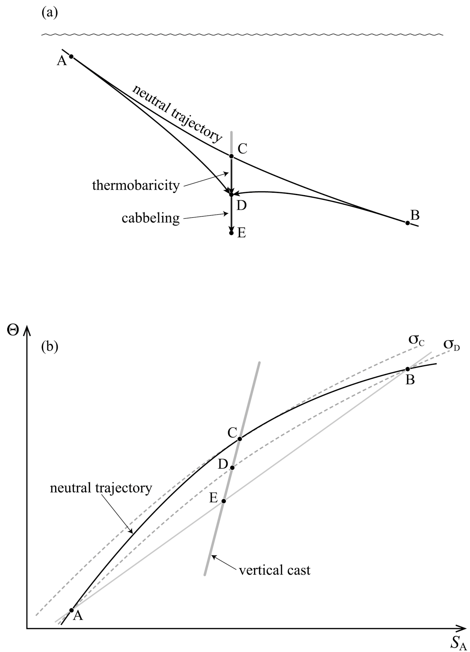
The thermobaric and cabbeling dianeutral advection processes are illustrated in Figure 1. Water parcels A and B are brought together in an adiabatic and isohaline manner until they meet at location D. During this adiabatic advection process their values of Absolute Salinity and Conservative Temperature are constant, and since we arranged that they meet at the location D, they must have the same value of potential density with respect to the pressure of location D, , (see this isopycnal on panel (b) of the figure); that is,
During this adiabatic and isohaline motion, parcel A moves through the ocean on the ocean’s specific volume anomaly surface ; that is, along the path through space that parcel A takes, the surrounding ocean’s Absolute Salinity and Conservative Temperature satisfy
while parcel B moves through the ocean surrounded by ocean whose Absolute Salinity and Conservative Temperature satisfy
During this adiabatic and isohaline motion, both parcels A and B fall off the neutral trajectory that links the original positions of the parcels in Figure 1a. This vertical motion occurs because these parcels have different compressibilities to the water on the neutral trajectory (because they have different temperatures and salinities to the corresponding parcels on the neutral trajectory). When parcels A and B mix with one another (in the appropriate mass ratio) they produce water parcel E which lies on the straight line joining parcels A and B on the diagram of Figure 1b. This mixing process has assumed that Absolute Salinity and Conservative Temperature are conserved during the turbulent mixing process. Once parcels A and B mix intimately (at the location D, but not with the ocean properties at this location), the density of the mixed parcel is greater than that of the original parcels and so the combined parcel sinks vertically from location D to location E. This sinking is due to cabbeling, that is, it is due to the potential density surfaces being curved on the diagram.
References
- Iselin, C.O’.D. The influence of vertical and lateral turbulence on the characteristics of the waters at mid-depths. EOS Trans. Am. Geophys. Union 1939, 20, 414–417. [Google Scholar] [CrossRef]
- McDougall, T.J. Neutral surfaces. J. Phys. Oceanogr. 1987, 17, 1950–1964. [Google Scholar] [CrossRef]
- McDougall, T.J. Thermobaricity, cabbeling, and water-mass conversion. J. Geophys. Res. 1987, 92, 5448–5464. [Google Scholar] [CrossRef]
- Griffies, S.M. Fundamentals of Ocean Climate Models; Princeton University Press: Princeton, NJ, USA, 2004; 518 pp + xxxiv. [Google Scholar]
- McDougall, J.T.; Jackett, D.R. The material derivative of neutral density. J. Mar. Res. 2005, 63, 159–185. [Google Scholar] [CrossRef]
- McDougall, T.J.; Groeskamp, S.; Griffies, S.M. On geometrical aspects of interior ocean mixing. J. Phys. Oceanogr. 2014, 44, 2164–2175. [Google Scholar] [CrossRef]
- Tailleux, R. Neutrality versus materiality: A thermodynamic theory of neutral surfaces. Fluids 2016, 1, 32. [Google Scholar] [CrossRef]
- McDougall, T.J.; Griffies, S.M.; Groeskamp, S. The direction of mesoscale eddy-induced lateral mixing in the ocean. J. Phys. Oceanogr 2017. submitted for publication. [Google Scholar]
- Valladares, J.; Fennel, W.; Morozov, E.G. Replacement of EOS-80 with the International Thermodynamic Equation of Seawater-2010 (TEOS-10). Deep-Sea Res. I 2011, 58, 978. [Google Scholar]
- IOC (International Olympic Committee), SCOR and IAPSO. The International Thermodynamic Equation of Seawater—2010: Calculation and Use of Thermodynamic Properties. Available online: http://www.TEOS-10.org (accessed on 25 April 2017).
- Turner, J.S. Buoyancy Effects in Fluids; Cambridge University Press: Cambridge, UK, 1973; 368p. [Google Scholar]
- Groeskamp, S.; Zika, J.D.; McDougall, T.J.; Sloyan, B.M.; Laliberté, F. The representation of ocean circulation and variability in thermodynamic coordinates. J. Phys. Oceanogr. 2014, 44, 1735–1750. [Google Scholar] [CrossRef]
- Veronis, G. The role of models in tracer studies. In Numerical Models of Ocean Circulation; National Academy of Science: Washington, DC, USA, 1975; pp. 133–146. [Google Scholar]
- Gargett, E.A.; Osborn, T.R.; Nasymyth, P.W. Local isotropy and the decay of turbulence in a stratified fluid. J. Fluid Mech. 1984, 144, 231–280. [Google Scholar] [CrossRef]
- Gregg, M.C.; Sanford, T.B. The dependence of turbulent dissipation on stratification in a diffusively stable thermocline. J. Geophys. Res. 1988, 93, 12381–12392. [Google Scholar] [CrossRef]
- McDougall, T.J. The vertical motion of submesoscale coherent vortices across neutral surfaces. J. Phys. Oceanogr. 1987, 17, 2334–2342. [Google Scholar] [CrossRef]
- McDougall, T.J. Neutral-surface potential vorticity. Prog. Oceanogr. 1988, 20, 185–221. [Google Scholar] [CrossRef]
- McDougall, J.T.; Jackett, D.R. On the helical nature of neutral trajectories in the ocean. Prog. Oceanogr. 1988, 20, 153–183. [Google Scholar] [CrossRef]
- McDougall, J.T.; Jackett, D.R. The thinness of the ocean in space and the implications for mean diapycnal advection. J. Phys. Oceanogr. 2007, 37, 1714–1732. [Google Scholar] [CrossRef]
- Klocker, A.; McDougall, T.J. Influence of the nonlinear equation of state on global estimates of dianeutral advection and diffusion. J. Phys. Oceanogr. 2010, 40, 1690–1709. [Google Scholar] [CrossRef]
- Klocker, A.; McDougall, T.J. Quantifying the consequences of the ill-defined nature of neutral surfaces. J. Phys. Oceanogr. 2010, 40, 1866–1880. [Google Scholar] [CrossRef]
- Iudicone, D.; Madec, G.; McDougall, T.J. Water-mass transformations in a neutral density framework and the key role of light penetration. J. Phys. Oceanogr. 2008, 38, 1357–1376. [Google Scholar] [CrossRef]
- Groeskamp, S.; Abernathey, R.P.; Klocker, A. Water mass transformation by cabbeling and thermobaricity. Geophys. Res. Lett. 2016, 43, 10835–10845. [Google Scholar] [CrossRef]
- Klocker, A.; McDougall, T.J.; Jackett, D.R. A new method for forming approximately neutral surfaces. Ocean Sci. 2009, 5, 155–172. [Google Scholar] [CrossRef]
- McDougall, J.T.; Klocker, A. An approximate geostrophic streamfunction for use in density surfaces. Ocean Model. 2010, 32, 105–117. [Google Scholar] [CrossRef]
Figure 1.
Sketch illustrating the two dianeutral advection processes, thermobaricity and cabbeling. Panels (a) and (b) show a neutral trajectory and a vertical cast in physical space and in space, respectively. The Absolute Salinity and Conservative Temperature of the ocean’s environment at the locations A–E in panel (a), are depicted in panel (b). When parcels A and B mix with one another (in the appropriate mass ratio) they produce water parcel E. This mixing between parcels A and B occurs at the pressure of point D, but the mixing occurs between parcels A and B and not with the ocean properties at this location. The potential density surface of parcel D with respect to the pressure at point D, is shown.
© 2017 by the authors. Licensee MDPI, Basel, Switzerland. This article is an open access article distributed under the terms and conditions of the Creative Commons Attribution (CC BY) license (http://creativecommons.org/licenses/by/4.0/).
Share and Cite
MDPI and ACS Style
McDougall, T.J.; Groeskamp, S.; Griffies, S.M. Comment on Tailleux, R. Neutrality versus Materiality: A Thermodynamic Theory of Neutral Surfaces. Fluids 2016, 1, 32. Fluids 2017, 2, 19. https://doi.org/10.3390/fluids2020019
AMA Style
McDougall TJ, Groeskamp S, Griffies SM. Comment on Tailleux, R. Neutrality versus Materiality: A Thermodynamic Theory of Neutral Surfaces. Fluids 2016, 1, 32. Fluids. 2017; 2(2):19. https://doi.org/10.3390/fluids2020019
Chicago/Turabian StyleMcDougall, Trevor J., Sjoerd Groeskamp, and Stephen M. Griffies. 2017. "Comment on Tailleux, R. Neutrality versus Materiality: A Thermodynamic Theory of Neutral Surfaces. Fluids 2016, 1, 32" Fluids 2, no. 2: 19. https://doi.org/10.3390/fluids2020019