
High Wavenumber Coherent Structures in Low Re APG-Boundary-Layer Transition Flow—A Numerical Study

School of Civil and Environmental Engineering, Nanyang Technological University, Singapore 639798, Singapore
*
Author to whom correspondence should be addressed.
Fluids 2017, 2(2), 21; https://doi.org/10.3390/fluids2020021
Submission received: 27 February 2017
/
Revised: 13 April 2017
/
Accepted: 18 April 2017
/
Published: 28 April 2017
(This article belongs to the Special Issue Turbulence: Numerical Analysis, Modelling and Simulation)
Abstract
:This paper presents a numerical study of high wavenumber coherent structure evolution in boundary layer transition flow using recently-developed high order Combined compact difference schemes with non-uniform grids in the wall-normal direction for efficient simulation of such flows. The study focuses on a simulation of an Adverse-Pressure-Gradient (APG) boundary layer transition induced by broadband disturbance corresponding to the experiment of Borodulin et al. (Journal of Turbulence, 2006, 7, pp. 1–30). The results support the experimental observation that although the coherent structures seen during transition to turbulence have asymmetric shapes and occur in a random pattern, their local evolutional behaviors are quite similar. Further calculated local wavelet spectra of these coherent structures are also very similar. The wavelet spectrum of the streamwise disturbance velocity demonstrates high wavenumber clusters at the tip and the rear parts of the Λ-vortex. Both parts are imbedded at the primary Λ-vortex stage and spatially coincide with the spike region and high shear layer. The tip part is associated with the later first ring-like vortex, while the rear part with the remainder of the Λ-vortex. These observations help to shed light on the generation of turbulence, which is dominated by high wavenumber coherent structures.
1. Introduction
The transition of the boundary layer from laminar to turbulent flow has attracted research interest for more than a century as it plays an important role in both fundamental studies of fluid mechanics and in engineering applications [1]. In this transition process, relatively small environmental disturbances introduced into the flow may amplify, interact with other nonlinear modes and lead to laminar flow breakdown. During the initial receptivity stage, the small amplitude disturbances are transformed into internal unstable Tollmien–Schlichting (TS) waves within the boundary layer [2]. If the TS waves amplify to sufficient amplitude [3], strong non-linear effects become significant and generate a series of two-dimensional (2D) harmonic waves resonantly [4]. As an enhancement of non-linear interaction, the harmonic waves are unstable to infinitesimal three-dimensional (3D) broadband disturbances that are always present both naturally and in experiments [5]. Based on their interacting mechanism, the normal transition can be subdivided into two kinds: fundamental transition first observed in [6] or subharmonic transition first discovered in [7].
In fundamental resonance, the TS wave interacts with the 3D disturbance wave of a given spanwise periodicity, resulting in an overall 3D structure with a “peak and valley distribution” in the spanwise direction for the streamwise disturbance velocity [6]. Λ-vortices in an aligned pattern appearing with tips at the peak positions when the 3D disturbance amplitudes have attained a magnitude of comparable order as the 2D TS wave.
Λ-vortices also occur in the subharmonic resonance, but are formed in a different way. The 3D structures are initiated by a 2D fundamental TS wave with frequency and its spanwise subharmonic wave with frequency [8]. The subharmonic wave rapidly amplifies to reach a magnitude of the order of the TS wave and leads to distortion in the spanwise direction [9]. Then, groups of weak Λ-vortices are formed in a staggered pattern.
In [9], the authors showed experimentally that, in the late stage of transition flow, the local behavior of the disturbances in the vicinity of -structures is very similar with regard to both fundamental and subharmonic resonances. The main common features of the transition process include: (a) the formation of -structures; (b) the appearance of spikes (large negative streamwise disturbance velocity in the time series) near the tips of -structures; and (c) the formation of ring-like vortices departing away from the -vortex and moving upward in the external part of the boundary layer. Although the physical observations of transition have been widely recorded in the literature [6,9,10], little consensus has been reached on a common mechanism behind the transition. In the experiments of [11], an Adverse-Pressure-Gradient (APG) boundary layer transition is induced by a TS wave plus initially weak broadband disturbances. The observed -vortices, intensive -shape high shear (HS) layers, -vortices, ring-like vortices and associated spikes seen in time-traces and other phenomena are distributed randomly in time and space and have somewhat distorted shapes. However, it is reported that their general properties are qualitatively similar across sub-harmonic, harmonic and broadband disturbances.
Since the local behaviors of the vortex are quite similar in the late stage of transition, there is a strong interest in a theory to explain the common features of vortex evolution. In [10], the authors found that the first sign of randomness in the transition process was observed at a position corresponding to the tip of the Λ-vortex. In an experimental study of [12], a 3D Soliton-like Coherent Structures (SCS), essentially a wave packet accompanied with a high shear layer, is proposed to be the building block of the vortical coherent structures, which leads to turbulent burst [11]. Similarly, the Direct Numerical Simulation (DNS) results of [13] indicated that turbulence is not generated by vortex breakdown, but rather by positive and negative spikes and consequent high shear layers. A follow-on study by [14] further proposed that the shear layer instability is the “mother of turbulence”. Both studies proposed theories suggesting a universal mechanism for turbulence generation and sustainment in [12,14]. Though different theories exist, the transition processes are essentially based on the existence of coherent flow structures and the formation of high wavenumber components, which is the precursor of turbulence. Therefore, the present study directly applies a local wavenumber detector, wavelet analysis to investigate the relationship between the typical vortical structure and the high wavenumber components, which is captured by a high order combined compact difference scheme in numerical simulations [15,16]. It can be shown that the local high wavenumber components in the streamwise direction mainly cluster inside the high shear layer region. The authors observe such behavior across fundamental, subharmonic resonance and transition induced by the broadband disturbance. The last case is the most general scenario, and hence, it is the focus of the present study.
Numerical simulation provides a helpful tool to investigate how spatial disturbance signals evolve temporally. Such studies have provided significant results to the study of boundary layer transition [10,17,18,19,20], but only a few of them present a spatial spectrum of the disturbance as in this study. The present study uses recently-developed high order combined compact difference schemes with non-uniform grids for numerical simulations of the Navier–Stokes (NS) equations for flat plate boundary layer transitions [15,16,21]. While these schemes are “DNS-like”, they however are highly optimized for boundary layer transitions, i.e., having (a) low-numerical dispersion/dissipation to preserve wave speed and amplitude, (b) non-uniform gridding in the wall-normal direction to capture the high velocity gradients near the wall and (c) reported good comparisons with the experiments of [22] for Zero-Pressure-Gradient (ZPG) and [23] for APG for (Reynolds number based on displacement thickness ) up to 1200. In the present study, simulation results of the experiments from [11] on the APG boundary layer transition with up to 1130 are analyzed in detail. Furthermore the Continuous Wavelet Transform (CWT) is used as the signal identifier to demonstrate the local high wavenumber spectrum in the boundary layer transition. This technique has been used to investigate turbulence by many researchers, e.g., in [24], the authors used wavelet analysis to demonstrate the Richardson cascade in turbulent flow.
The organization of this paper is as follows: Section 2 gives a brief description of the Combined Compact Difference (CCD)-based numerical model used to simulate the experiment of [11] on APG boundary layer transition. Section 3 makes a qualitative comparison between the simulation results and the experiment. It demonstrates the common features of the vortex in the boundary layer across fundamental and subharmonic transition also existing in broadband disturbance. Section 4 discusses the application of CWT to analyze transition signals demonstrating that CWT is a good identifier of high wavenumber components in transition flow. Section 5 tracks the evolution of a typical Λ-vortex showing that the high wavenumber components are imbedded in the associated spike region, and high shear layers developed in transition boundary layer flow. Section 6 provides the conclusion.
2. Numerical Model
In the numerical model of the boundary layer flow used here, all variables in the Navier–Stokes equation are expressed in non-dimensional form and related to their dimensional counterparts, denoted by bars or uppercase, as follows:
where , and denote the coordinates of streamwise, wall-normal and spanwise direction, respectively, and , , are the corresponding velocity components in each direction, is the characteristic length, is the freestream velocity, is the kinematic viscosity and is a reference Reynolds number. , , and are used to denote the corresponding dimensional spatial and temporal coordinates. The NS equations are solved using a vorticity-velocity formulation with corresponding vorticity components in non-dimensional form given as:
In addition, the total flow field is decomposed into a steady 2D base flow and an unsteady 3D disturbance flow , which is expressed as:
with:
2.1. Computational Domain
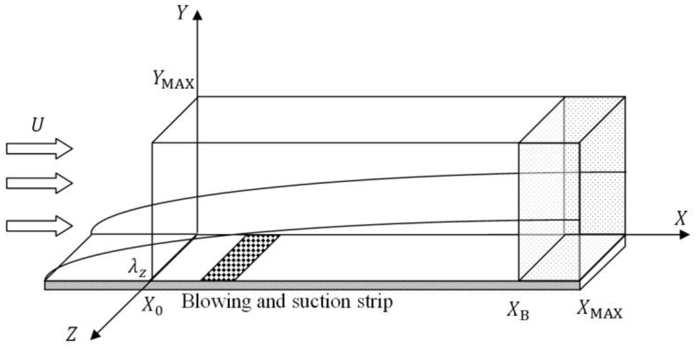
The computational domain was setup to closely match the experimental environment of [11]. The physical system is that of an APG boundary layer flow (with Hartree parameter = −0.115) over a flat plate, which is disturbed by a blowing and suction strip at a certain upstream location. A comparison sketch of the distance from leading edge, disturbance source location and main region of interest along the streamwise direction are sketched in Figure 1. The rectangular computational domain is shown schematically in Figure 2. The computational domain is 500 mm × 25.3 mm × 48 mm in the streamwise (), wall-normal () and spanwise () directions, respectively, and started at 250 mm from the leading edge. The blowing and suction strip was located over 287 mm to 308 mm to simulate the disturbance sources used by [11]. The amplitude of the disturbances were calibrated to that at location X = 450 mm using available experimental results. The main region of interest was over X of 450 mm to 530 mm where experimental data are reported, even though the experimental section continued to 1490 mm. The present computational domain, though smaller, covers this region of interest and extends to X = 580 mm, after which a buffer domain was used until X = 753 mm.
The length of the domain in the wall-normal direction in the simulation covers about 12-times boundary layer displacement thickness , with typical turbulent structures extending upwards to 5. Thus, there is no suppression of turbulence development. The measured disturbance signals in the experiment repeats every 48 mm in the spanwise direction; hence, the spanwise domain size used here is one disturbance wavelength, of 48 mm.
2.2. Simulation of Base Flow
The steady base flow solution was first obtained from numerical integration of the NS equations to a steady state:
At the inflow boundary, the solution of the Falkner–Skan equation was used to specify the base flow variables. No-slip and no-penetration conditions were used at the wall. The wall vorticity was calculated from the velocity field considering the continuity condition. The vorticity vanished at the freestream boundary where was prescribed as:
where the form of is given later in Section 3.
At the outflow boundary, all equations were solved dropping the second -derivative terms, and is calculated from:
A more detailed description of these boundary conditions in a Blasius boundary layer flow is found in [15].
2.3. Simulation of Base Flow
The NS equations consist of three vortex transport equations:
where:
and three velocity Poisson Equations [19,25]:
All disturbance flow variables vanished at the inflow boundary. Potential flow held at the freestream boundary so that the vorticity components vanished. Equations (18) and (20) were solved for and at the freestream boundary. For , the local wall-normal gradient was prescribed to impose an exponential decay [26]:
where and and are the streamwise and spanwise wavenumbers, respectively.
At the wall boundary, no-slip conditions were used. The vorticity components were calculated from their relationship with velocity [19,26,27]. A buffer domain method was used at the outflow boundary to allow disturbances to travel out of the computational domain without upstream reflection. Periodicity conditions were employed at the spanwise boundaries at = 0 and = . Centerline symmetry is not assumed here, unlike, e.g., other reported work [19,26,27], so that the asymmetric disturbance waves could develop freely.
2.4. Numerical Method
Since the unsteady disturbance flow was assumed to be spanwise periodic, the disturbance flow variables and the terms were expanded using Fourier modes:
where and is the lowest spanwise Fourier mode, which is related to the spanwise wavelength by:
Substituting Equation (22) into Equations (12) to (20) gave a set of governing equations for each -plane integration domain. The nonlinear terms , and of the vorticity transport equations were evaluated pseudo-spectrally using fast Fourier transform for conversion from Fourier space to physical space and back with the 3/2 rule used for de-aliasing [28].
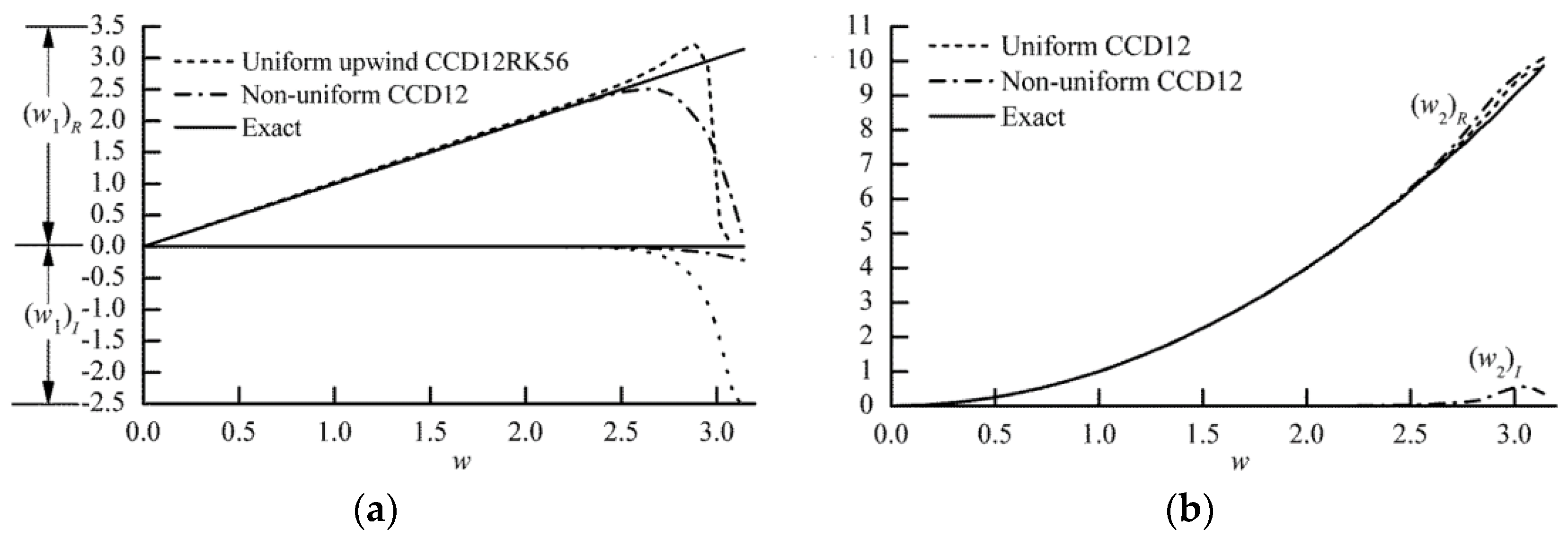
Combined Compact Difference (CCD) schemes up to 12th-order accuracy were used in the streamwise and wall-normal directions as reported in [15,16]. The spectral resolution of these schemes can be demonstrated by the modified wavenumber analysis following [29], wherein the scaled wavenumber where is the physical wavenumber and is the grid spacing. The modified scaled wavenumber i.e., the one represented by the finite difference scheme, is typically complex. The closer is to , the more accurate is the scheme. The modified wavenumber analysis for each scheme used in the simulation is presented in Figure 3. The upwind CCD scheme co-optimized with fourth order 5 to 6 alternating stage Runge–Kutta (RK) scheme (denoted as uniform upwind CCD12RK56 in Figure 3a) was used for the term in Equations (12) to (14) and (18) to (20) in order to preserve low-dispersion (related to the real part of ) and low-dissipation errors for wave propagation (related to the imaginary part of ). This scheme also suppressed numerical oscillations introduced from the buffer domain, because of the very negative near = 3. The terms in Equations (12) to (14) and (18) to (20) are discretized with a centered difference scheme (denoted as uniform CCD12 in Figure 3b) [15]. In the wall-normal direction, the CCD schemes were directly constructed on a non-uniform grid without the use of coordinate transform. The spectral resolution for the non-uniform CCD12 scheme used for is given in Figure 3a, and that for is given in Figure 3b. A second-order 5 to 6 alternating stage Strong Stability Preserving (SSP) RK scheme was used for the term to allow a larger time step. All of the schemes presented in Figure 3 have a high spectral resolution up to = 2.5, and detailed analyses of these schemes are given in [15,16]. A multigrid method is used to solve the velocity Poisson Equation (19). A stable stretching grid [16] was used in the direction to obtain fine resolution in the near-wall region.
In the present simulations, 1000 uniform grid points with = 0.5 mm were used in the streamwise direction, which represented a resolution of about 61 grid points per TS wavelength. Since 12th-order CCD schemes was used in this direction, a scaled wavenumber as high as 2.5 could be accurately simulated, implying that harmonic waves with the wavenumber roughly 25-times the TS wave could be accurately captured [15]. Considering that the TS scaled wavenumber in the present simulation is 0.103 (TS wavenumber × = 205.9 rad/m × 0.5 × 10⁻³ m), the highest wavenumber that can be accurately resolved is thus about 5000 rad/m (205.9 rad/m × 2.5/0.103). In the wall-normal direction, 120 grid points were used. A stable stretching grid was used in the near-wall region with grid sizes ranging from 0.01 to 0.62 mm. This had been demonstrated to successfully resolve the large velocity gradient of the high shear layer in the boundary layer transition flow [16]. Sixteen Fourier modes were used in the spanwise direction. The total number of grid points used in this study was 3.84 × 10⁶. was selected to be as small as 6.56 × 10⁻⁶ s so that the maximum CFL number in the streamwise direction () 0.12, which satisfied the scheme optimization condition given in [15]. This also satisfied the stability criterion in the wall-normal direction as detailed in [16]. As all variables were non-dimensionalized in Equation (1), the needed kinematic viscosity used was 1.526 × 10⁻⁵ m2/s, as in the experiments by [11]. The reference velocity was selected to be = 30.52 m/s. The reference length was set as 0.05 m, so that the reference Reynolds number is 105. The local Reynolds number based on displacement thickness ranged from 820 to 1130 over the computational domain.
It is noted that the number of grid points in the present simulation (1000 streamwise × 120 wall normal × 32 spanwise) would usually be insufficient to resolve the full-scale vortex motion even in this low-Reynolds number turbulent boundary layer when using lower resolution schemes. As a comparison, a similar study on fundamental resonance using Direct Numerical Simulation (DNS) in [19] on the ZPG transition flow up to the stage where the -vortex was formed used fourth order finite difference schemes on a grid of 3000 (streamwise) × 65 (wall-normal) × 32 (spanwise). The highest wavenumber disturbances dominated in the streamwise direction necessitating finer grid point in this direction. In [30] where a second order finite difference scheme in each direction was used, typically 4096 × 400 × 128 grids were needed to simulate a fully-developed turbulent boundary layer. Here, the use of 12th order CCD schemes allowed the grid points in the streamwise direction to be significantly reduced. In particular for the experiment of [11], which the present results are being compared to, the highest disturbance frequency recorded is around 1100 Hz (Figure 19 in [11]). Since the TS wave frequency is 109.1 Hz, this means about 10 harmonics of TS wave exist. As the TS wave number is 205.9 rad/m, hence the wavenumber of the 10th harmonic is 2059 rad/m. Considering that the amplitude of broadband disturbance is comparable with the harmonics of TS wave, the disturbance should thus be resolved by the present numerical scheme with resolution up to 5000 rad/m. The flow parameters, grid resolution and size of the computational domain are summarized in Table 1.
The preceding analysis shows that the present resolution can capture the major vortical motion during the transition. Further as the present study is on an APG boundary layer and also focuses on mid-stage including ring-like vortices formed after -vortices, the velocity gradients in the wall-normal direction are larger than in [19], necessitating the stretching grid with higher resolution in the near-wall region. The comparison with experiments from [11] as given below demonstrates that grid used was sufficient to resolve the dynamics of the most energetic vortices, enabling the numerical simulation to realistically model the vortex evolution in the transition flow experiment.
2.5. Continuous Wavelet Transform
The CWT used to investigate the evolution of coherent structures is described next. The CWT is defined as:
where is the mother wavelet and is the scale of the transform and can be determined by:
is the centered frequency of the wavelet; is the wavenumber spectrum of the signal; and is the grid space or sampling period.
The most commonly-used wavelet is the complex-valued Morlet wavelet because it gives information on the phase and has good resolution for the high wavenumber components [31]. The complex-valued Morlet wavelet used here is given by:
where is the non-dimensional frequency, taken to be six, as in [32].
2.6. Excitation of Disturbance Waves
The disturbance waves in experiment of [11] were produced by blowing and suction of air through a slit with point-like sources on the flat-plate surface perpendicular to the flow direction and located at distance = 300 mm from the leading edge. The disturbance signals consisted of two main components: the signal corresponding to the fundamental 2D TS wave and broadband 3D pseudorandom small-amplitude signals (“noise” of the TS wave). The broadband signals have approximately the same amplitudes in the frequency spectrum, but different phases for the spectral modes. The broadband signals repeat in the spanwise direction with a period of 48 mm.
In the present simulation, the disturbances are introduced from the wall-normal velocity component in the spanwise spectral space. The TS wave is generated by:
where is the disturbance frequency and is 109.1 Hz, is the random signal, discussed later, and is used to adjust the amplitude to make the r.m.s. streamwise velocity (maximum in ) equal to around 4% of the freestream velocity at = 450 mm. It is noted that this is a relatively large amplitude so that the broadband disturbance wave can develop nonlinearly even at the initial stage and trigger vortex formation in a shorter distance downstream. This is so that a smaller computational domain can be used. However this amplitude should not be too large as to distort the base flow. This selection of the initial amplitude follows that used in the experiment (see Section 2.8 for a validation) where similar arguments are used to justify the initial amplitude.
The spatial dependence was introduced via the disturbance distribution function developed in the present study. It is selected to satisfy the following three conditions:
- Disturbances start and end with zero amplitude: .
- No discontinuity for the first derivative at the beginning and the end of the strip, i.e.,
- The form is conservative, so that .
Conditions (1) and (2) make the transition from disturbance source to the wall smooth, while Condition (3) enforces the law of mass conservation to the imposed disturbances. One possible choice that is used here is:
The shape is shown in Figure 4.
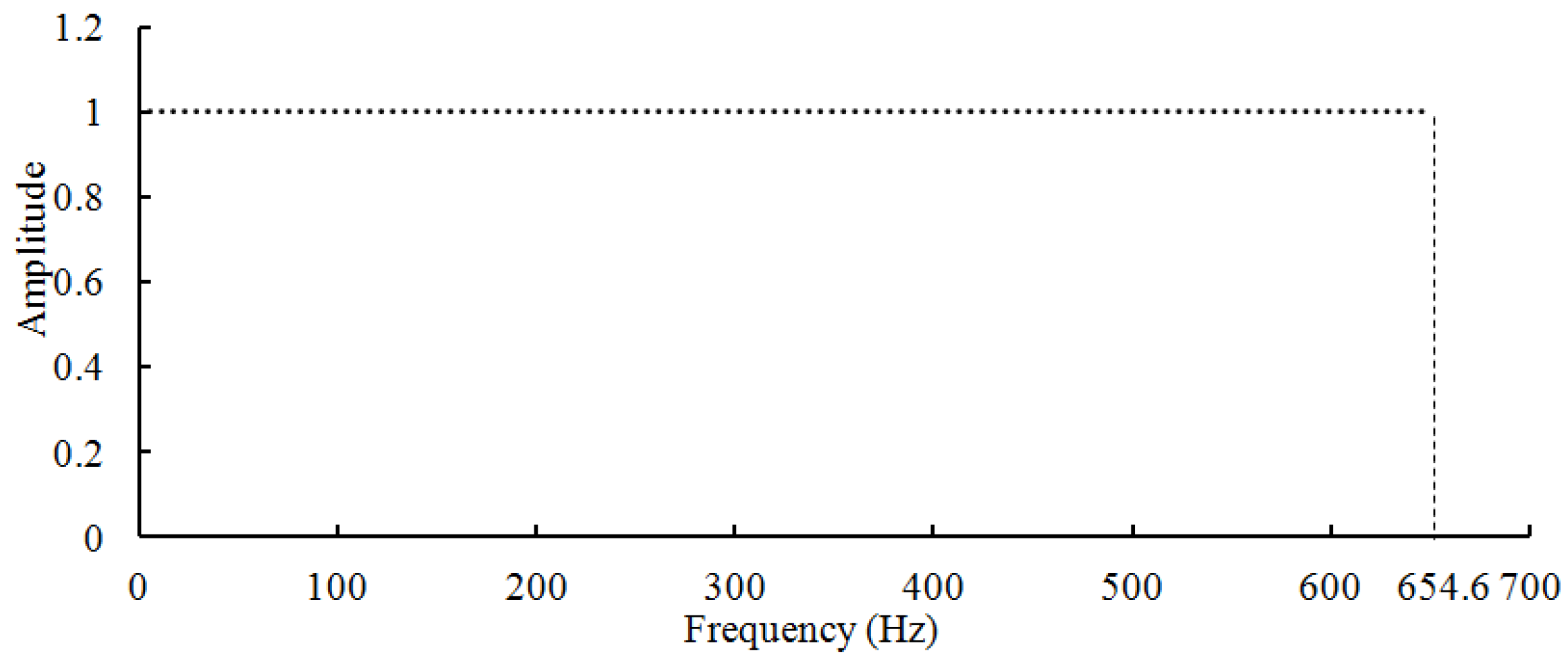
The randomized disturbance in Equation (27) is first generated in the Fourier space with the frequency band up to six-times the TS wave. The inverse Fourier transform is used to recover the signal in the time space as shown in Figure 5. This broad band signal has randomized phases, but the same normalized amplitude, as shown in Figure 6 for its spectrum. This signal amplitude is about 2% of of the fundamental TS wave (refer to Figure 6 in [11]). Besides in Equation (27), an additional 14 different signals were imposed on the real and imaginary parts of the Fourier modes , where = ±1, ±2, ±3,..., ±7. Thus, by construction, all of these spanwise Fourier modes have the same spectrum shown in Figure 6.
2.7. Code Validation
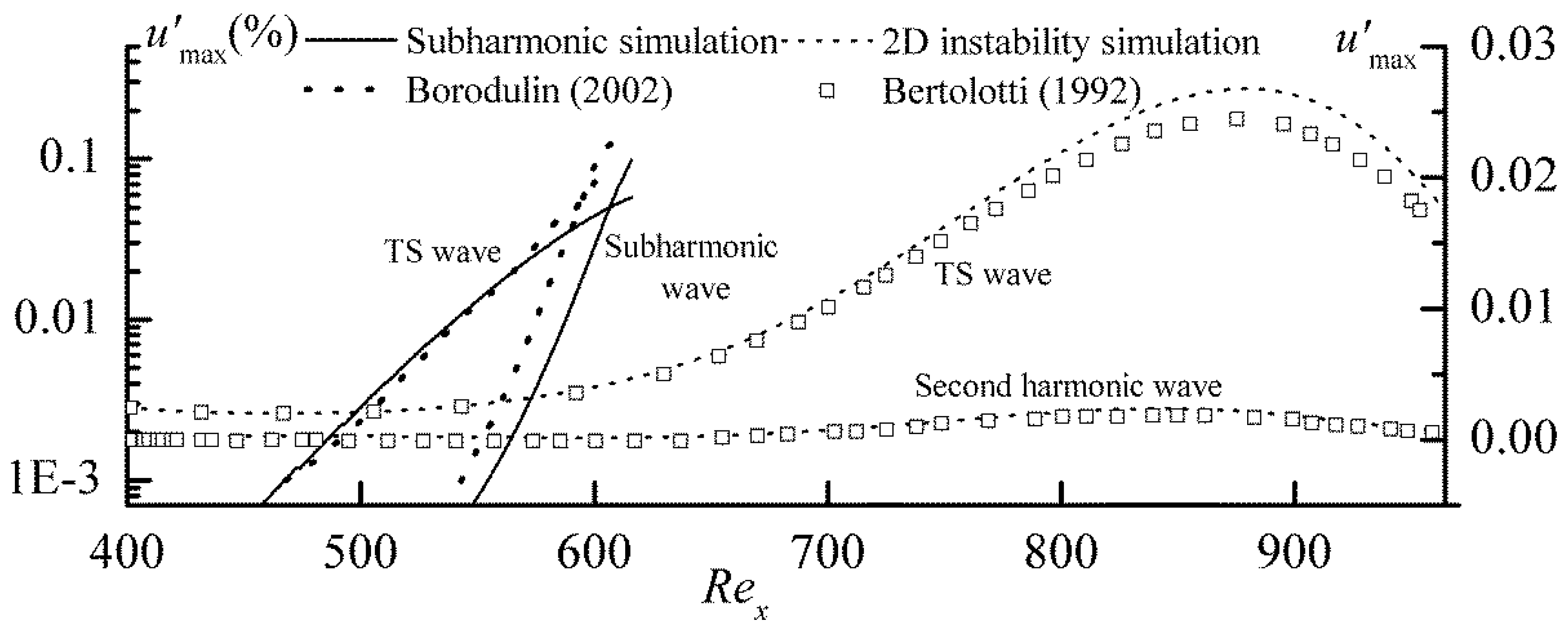
Since randomized disturbances are used in the present simulation of the experiment of [11], a direct quantitative comparison between the results is not possible. However, the subharmonic resonance experiment of [23] is very similar to the present case with the only difference being the source of disturbance. The comparison was reported earlier in [15] where the TS wave interacted non-linearly with the subharmonic wave, and the amplitude of the latter amplified dramatically along the downstream direction, as shown in Figure 7, where the streamwise disturbance amplitudes of different components are plotted against Reynolds number (the length scale refers to the distance from the leading edge). Although the simulated amplification of the subharmonic wave is slightly weaker than in the experiment, the agreement was generally good.
In addition, the CCD12RK56 scheme on the uniform grid is validated by simulating 2D amplification of the TS wave in [33]. As shown in Figure 7, the initial amplitude of TS wave is small, but as it amplifies, its second harmonic wave is triggered. The results compare well with [33]. More details are found in [15].
2.8. Comparison of Settings between Simulation and Experiment
Before further investigation of the coherent structures via the simulation, the simulation results are first compared with the experiment to calibrate for the initial conditions and base flow. The non-dimensional freestream velocity in Equation (10) is prescribed as:
where is the Hartree parameter fixed as −0.115 and is selected as 8.295 to match the freestream velocity gradient in the experiments of [11]. Detailed comparisons of the base flow are not presented here, but are found in [21], including comparisons of the streamwise distribution of freestream velocity, base flow velocity and the boundary layer displacement thickness.
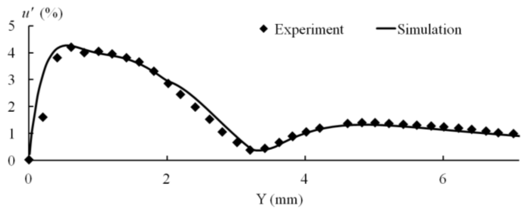
In [11], the disturbance flow is first measured at the initial section X = 450 mm. The initial amplitudes of the TS wave and broadband disturbances are adjusted to match the experimental condition at this location. The wall-normal profile of the TS wave amplitude at X = 450 mm is shown in Figure 8 along with the simulation showing that a good match was achieved.
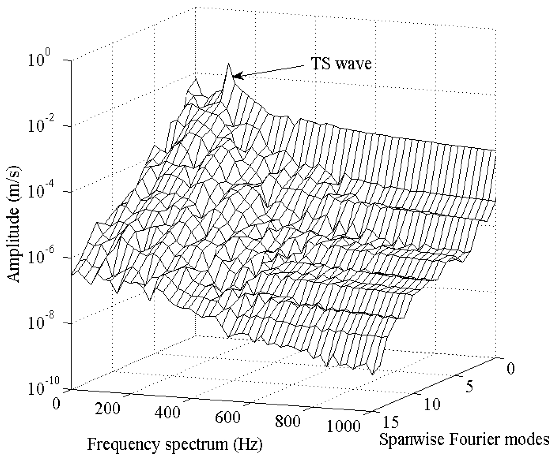
The wave amplitude spectrum plotted against frequency and spanwise Fourier modes is shown in Figure 9. The TS wave amplitude is dominant at a frequency of 109 Hz and spanwise Fourier Mode 0. The disturbance wave amplitudes decay with both the frequency and Fourier mode.
3. Overall Properties of Coherent Structures
Common shapes of the typical coherent structures in broadband disturbances are presented in this section to demonstrate the common features of coherent structures by streamwise velocity disturbance and the Q-criterion. The structures in broadband disturbances are further compared with those seen in the experimental results of [11].
3.1. Coherent Structures in Broadband Disturbance Flow
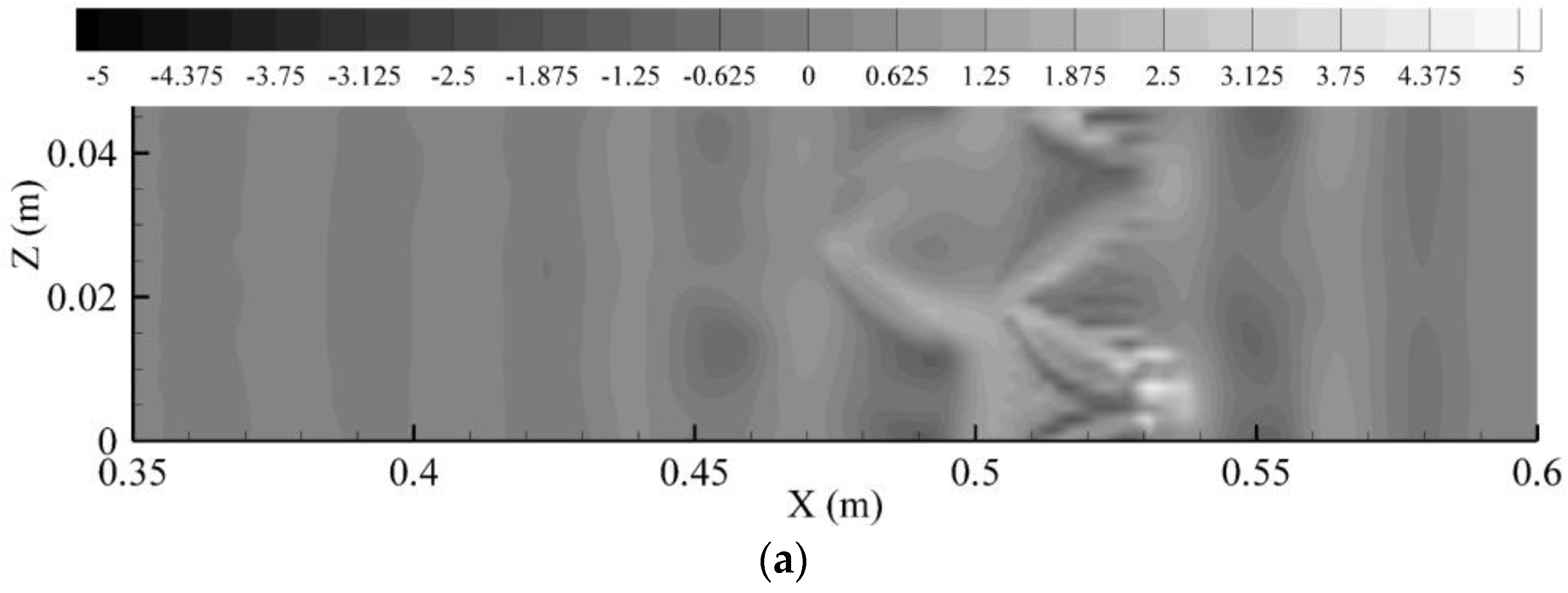
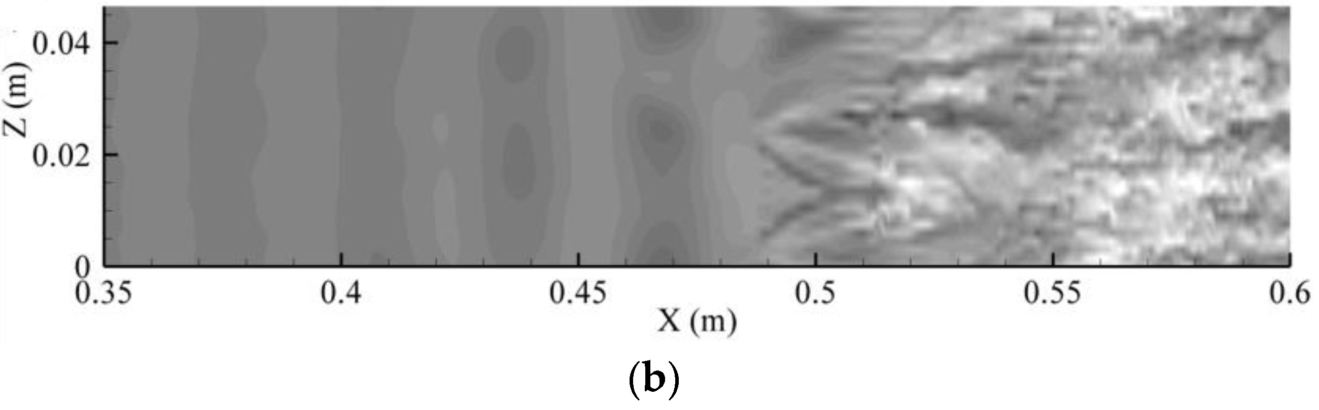
The process of coherent structures’ formation in broadband disturbance flow is shown in Figure 10a,b, which are contour plots of the streamwise disturbance velocity at Y = 1.2 mm with Figure 10a being at an early time stage and (b) at a later stage after the vortices have broken down. There is a weak spanwise flow distortion before X = 0.4 m, and localized structures are formed around X = 0.45 m. Both structures at X = 0.52 m (Figure 10a) and at X = 0.5 m (Figure 10b) show a shape that resemble the well-known -vortex observed in [10,19]. However, these structures arise in a random order, though the distances in the streamwise direction between these structures are roughly one TS wavelength. In Figure 10a, the structures are roughly arranged in an aligned pattern, which is the characteristic of fundamental resonance (see [8]). In Figure 10b, these structures are in a staggered pattern like the ones in subharmonic resonance (see [8]).
Visualization of vortices is performed using the iso-surface of the Q-criterion following [34], which is defined as a second invariant of the velocity gradient. While it focuses only on the rotational part of the vorticity at the expense of the strain, it is widely used for visualizing vortex structures in early-to mid-stage transition [30,34,35,36]. Chakraborty et al. [35] further compared several prevailing vortex identification criteria including the Q-criterion and concluded that all resulted in remarkably similar looking structures. The λ2-isosurface as an improved criterion was used in a recent transition study by Liu et al. [14], though Chakraborty et al. [35] indicated that the λ2-isosurface only captures the strain on a specific plane [37]. Since late stage vortex breakdown, after the formation of ring-like vortices, is not the focus here, using the Q-criterion for comparison of vortex development with experiments is sufficient, as the observed vortices are driven mainly by the rotational part. The strain is further examined via the wall region shear .
Figure 11 visualizes the vortices at two different times T showing that the vortices develop with different shapes and patterns. In Figure 11a, the vortex centered at Z = 0.01 m has developed into an -shape, while the one centered at Z = 0.04 m is still a primary -vortex. Similarly, in Figure 11b, a mature -vortex centered at Z = 0 m has formed and started to evolve to an -vortex, while the one centered at Z = 0.025 m has formed a ring-like vortex at its tip.
The vortex features shown in Figure 10 and Figure 11, and similar plots (not shown), indicate that broadband disturbances do not qualitatively change the typical -shape of the coherent structures. The effects of broadband disturbances on coherent structure formation are summarized as: (1) the coherent structures are spatially arranged in random order; and (2) at the same spatial location, the coherent structures may be in different evolution stages.
3.2. Spatial Shapes of Coherent Structures
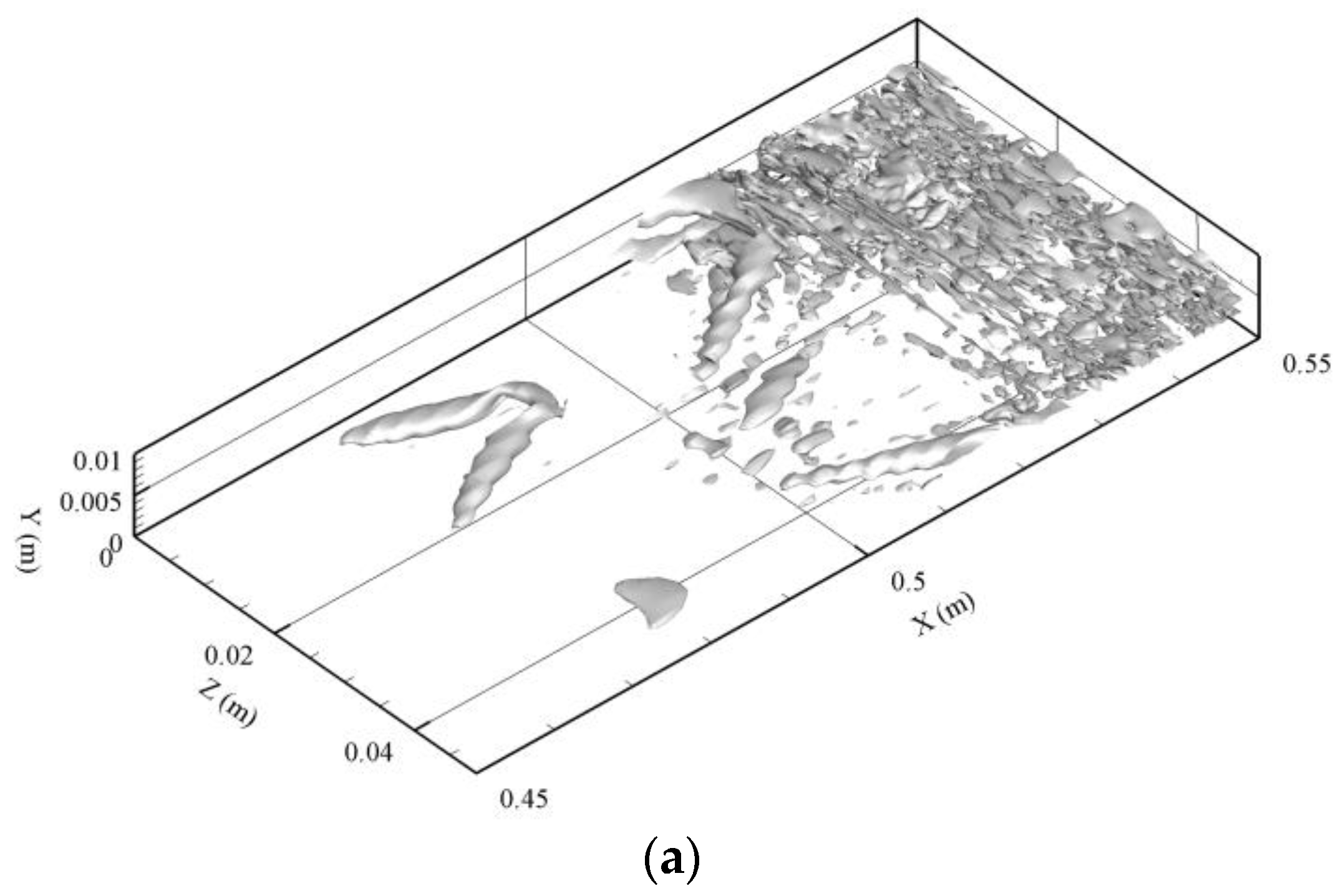
The typical spatial shapes of several individual coherent structures observed at around X = 0.49 m in the simulation are shown in Figure 12 by plotting the iso-surface of = −8% of freestream velocity. They have the common features of the coherent structures reported for fundamental and subharmonic resonance [11,9]: they are close to a -shape having two legs in the rear and one tip in the front. However, most of these structures are asymmetric due to the effects of broadband disturbances. In Figure 12a,d, one leg is longer than the other. There, the two structures are partially overlapped and merged in Figure 12b, while the coherent structure is close to symmetric in Figure 12c. The structure in Figure 12d is only at the beginning of its formation.
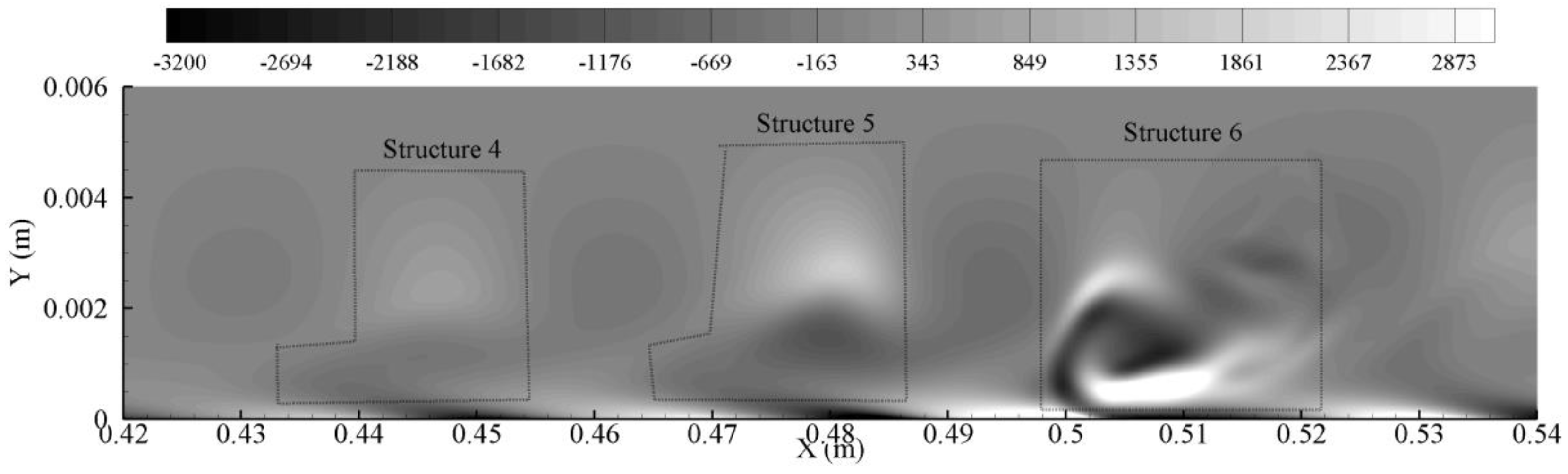
The further downstream development of the coherent structures at around X = 0.53 m is shown in Figure 13. It can be seen that the structures at this location have evolved to shapes qualitatively similar to the typical -vortex. Compared with Figure 12, these structures have stretched, becoming sharper in the streamwise direction and spread in the spanwise direction. The separation of the two legs has become clear with the tip starting to swell. Figure 13a shows a structure very similar to the typical symmetric -structure. The structures in Figure 13b,c evolve from those in Figure 12a,b, respectively. The asymmetry of both structures has become more obvious. The left leg of the structures has developed further than the right leg in Figure 13b (note that the part at Z = 0.045 m is the leg of another structure). The two legs of the two close structures have merged to a tail in Figure 13c,d showing a structure that only developed its left leg.
Figure 12 and Figure 13 fully demonstrate the polymorphism of coherent structures generated by broadband disturbances. However, all of the structures display qualitatively the same shape as the typical -vortex observed in boundary layer transition flow. This observation indicates that there may be common mechanisms that govern the coherent structure evolution.
Although the simulation results are not quantitatively comparable with the experiments of [11], the structure properties, including disposition and spatial shape, match the experimental results well (see Figure 17 and Figure 21 in [11]). The spatial shapes of vortical structure seen in the experiment are qualitatively similar to the ones found in the present simulation shown in Figure 12 and Figure 13. Therefore, it is concluded that the present simulation is able to sufficiently capture the effects of broadband disturbances on coherent structure evolution allowing further investigations using CWT on the computed results.
4. Characteristic Signal Pattern of Coherent Structures
The signal pattern from a transition flow experiment is usually analyzed using the time series of streamwise disturbance velocity [8,12], as it is experimentally easier to record the velocity at a certain location with a point probe than to record the entire velocity field. However, this is not a constraint in simulations. To further investigate the disturbance signal evolution, it is more insightful to analyze the spatial-temporal development of the disturbance signal, which can demonstrate how the high wavenumber components develop as the vortex evolves.
Flow structures with different shapes are shown in Figure 14 via the contour at Y = 1.18 mm and at T = 0.056 s. This particular time is chosen for discussion as the coherent structures exhibit a whole range of evolution behavior with random spatial locations and asymmetric shapes. Structures 1 and 4 are in their primary stage with rhombus-like shapes, where Structures 2, 3, 5 and 6 are in the developed stage with quasi-Λ-shapes.
Figure 15 presents the evolution of vortex visualized by the Q-criterion at T = 0.056 s. Structure 1 in Figure 14 has not developed a vortex, while Structure 4 forms a very weak primary Λ-vortex, which is a precursor of the well-known -vortex. Meanwhile, Structures 2 and 5 have developed to the stage of a quasi--vortex. Structure 3 has formed a -vortex with two asymmetric legs. Structure 6 has developed to a later stage when the first ring-like vortex has started to separate.
CWT is next performed on in the downstream direction. The highest wavenumber that CWT can resolve depends on the spectral resolution of the numerical scheme used. The present CCD scheme resolves the effective scaled wavenumber is up to 2.5, i.e., up to 5000 rad/m, as discussed earlier.
Figure 16a plots the streamwise disturbance velocity at T = 0.056 s, Y = 1.18 mm, Z = 13.5 mm, which goes through the spanwise centers of Structures 4, 5 and 6 in Figure 14. Figure 16b plots the corresponding wavelet contour in absolute amplitude (m/s) on the log10 scale so that the small-scale wave amplitudes are also seen. The energy at wavenumbers smaller than 500 rad/m mainly corresponds to the fundamental TS wave, subharmonic wave and the secondary harmonic wave with the wave energy continuously increasing along the downstream direction. The figure also shows energy peak structures at wavenumbers larger than 1000 rad/m, indicating a discontinuous energy distribution in this region. The peak structures are also amplifying with downstream distance. After X = 0.5 m, the energy at the high wavenumber is almost the same as in the low wavenumber.
The twin-peak region (demarcated by dashed lines in Figure 16) for Structure 4 extends from X = 0.436 m to 0.454 m, for Structure 5 from X = 0.468 m to 0.486 m and for Structure 6 from X = 0.498 m to 0.522 m. A comparison with Figure 14 and Figure 15 shows that these twin-peak regions coincided with the spatial region of the coherent structures. The two peaks of Structures 4 and 5 in Figure 16 are physically located very close so that the two peaks occurred within the one complete structure seen in Figure 15. For Structure 6, the two peaks are somewhat separated in Figure 16, and Vortex 6 in Figure 15 is just at the stage when the first ring-like vortex separates from -vortex. The two peaks with larger amplitude are spatially associated with these two vortices. Thus, the high wavenumber components in the wavelet spectrum are as expected spatially coincident with the coherent structures with a clustering of energetic high wavenumber components at the streamwise edge locations of the coherent structures.
The above discussion shows that as the coherent structures develop further downstream, the energy at high wavenumber becomes more prominent. Moreover, it indicates that prior to the formation of -vortex, the high wavenumber structure has already arisen upstream and is composed of two wave packets corresponding to the twin-peak CWT signals of the coherent structures in Figure 16. As the primary coherent structure evolves to the -vortex, the two wave packets are still spatially connected though amplified. At a further stage when the front wave packet becomes strong enough, it separates from the rear wave packet. In physical space, this corresponds to the separation of the first ring-like vortex from the -vortex. Here, we also note that the CWT results reflect the presence of subharmonic waves, specifically via a slightly high amplitude (lighter) band at a wavenumber around 100 rad/m over X= 0.46 to 0.54 m, while the harmonics of the TS wave are always present (the TS wave here has a wavenumber of 205.9 rad/m). Thus, both subharmonic and harmonic waves are generated.
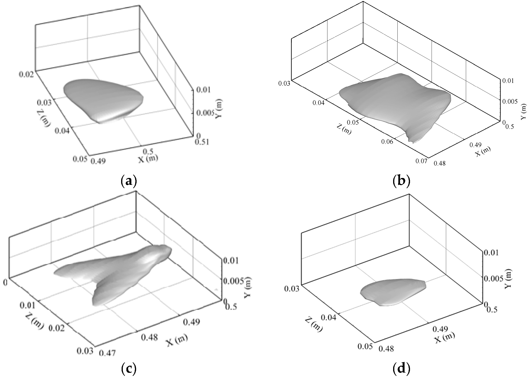
Figure 17 plots the contour of the shear at Z = 0.0135 m, i.e., the spanwise location is just around the centers of Structures 4, 5 and 6 shown in Figure 14. It can be seen that the high shear structures, especially for Structures 4 and 5 (the dark regions at round Y = 1 mm), coincide with the wavelet structure patterns in the streamwise direction shown in Figure 16. Therefore, the high wavenumber components are imbedded in the high shear layer structures near the wall. Details about the high shear structures are discussed in the next section. It is also noted that the high shear is the dominant component of spanwise disturbance vorticity during the transition stage discussed in this paper; the subsequent discussion focuses on and .
5. Coherent Structure Evolution
We now follow the full evolution process of a quasi-Λ-vortex, spike region, high shear layer and the high wavenumber components in the transition flow. Spike regions and high shear layers have been considered as important structures associated with turbulence generation [12,14]; hence, the wavelet spectrum is analyzed with these two structures. It is seen below that high wavenumber components have already developed at the primary stage of the Λ-vortex, spike region and high shear layer and evolve together with them. Further in the transition stage up to the formation of the first ring-like vortex, the high shear layer dominates the spanwise vorticity. To demonstrate this, a slightly asymmetric vortical structure is selected for convenience of comparison with the typical evolution process in subharmonic and fundamental resonance, as observed in [10,19,21,38], but without loss of generality.
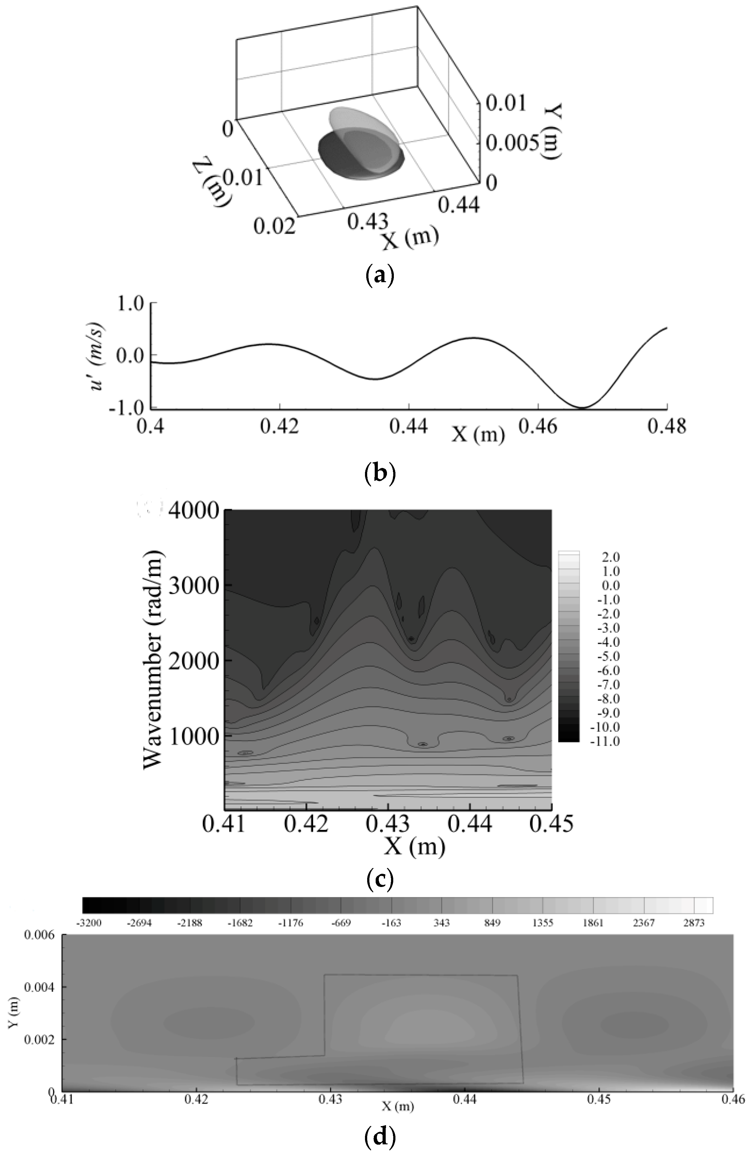
5.1. Spike Region and Primary -Vortex
As shown in Figure 16, the high wavenumber components mainly concentrate on the local minimum of the streamwise disturbance velocity, which is commonly referred to as a spike. Here, the spike region of Figure 11 is visualized in 3D by plotting the iso-surface of the streamwise disturbance velocity with about 60% of the local minimum around the coherent structure during a certain period. The 60% threshold value is chosen to have a clear 3D view of the local velocity distribution.
Figure 18a shows a visualization of the evolution of the spike region at its initial stage by plotting the iso-surface of = −0.4 m/s (57% of local minimum) at time T = 0.053 s along with the primary vortex visualized by the Q-criterion. In this early stage, the spike region comprising of a flat, rhombus-like structure located very close to the wall at around Y = 1.5 mm is seen. On top of the structure is a primary vortex, which evolves to the mature Λ-vortex further downstream location (see Figure 19).
It is illustrative to examine the spectral components of this structure to shed light on the development of later high wavenumber components. Figure 18b plots the disturbance though the center of the primary Λ-vortex, which spread from X = 0.425 to 0.442 m. The corresponding wavelet transform in Figure 18c over this X-range shows the expected two separated high wavenumber bursts at around X = 0.435 m, which is the spike location in Figure 18b. The energy of these two bursts is mainly concentrated at wavenumbers below 1000 rad/m.
The CWT results clearly show that the spike region defined here actually contains two wave packets even during this early stage. It is consistent with observation of Kachanov and Borodulin’s experiments [8,39] where two groups of high-frequency secondary fluctuations in the streamwise disturbance velocity time series were seen. The upper packet further from the wall corresponds to the first spike. Its early spectral view is shown in Figure 18c, and its physical view can be seen at a later time (in Figure 20c). The other packet (the rear peak in Figure 18c) close to the wall has velocity practically equal to the velocity of the high shear layer. This observation demonstrates the existence of the twin-wave packet structure at the stage before the formation of a strong spike. The present CWT result, consistent with experimental observations, shows the origin of these two wave packets as developing from the local valley of the approximately sine wave behavior of . At the present stage, even though the first spike that as typically associated with the first ring-like vortex has not yet fully developed, its characteristic spectrum has already formed via the front peak in the wavelet transform.
The last subplot in Figure 18 for shows the distribution of the high shear layer of this structure. turns from negative to positive as its distance increases from the wall. Near the wall, it stretches from X = 0.425 to 0.445 m, which approximately matches the distribution of the twin-peak distribution of the high wavenumber components in Figure 18c. Therefore, the high wavenumber components are already developed at the location of the wall high shear layer at this primary stage where the Λ-vortex is not yet mature.
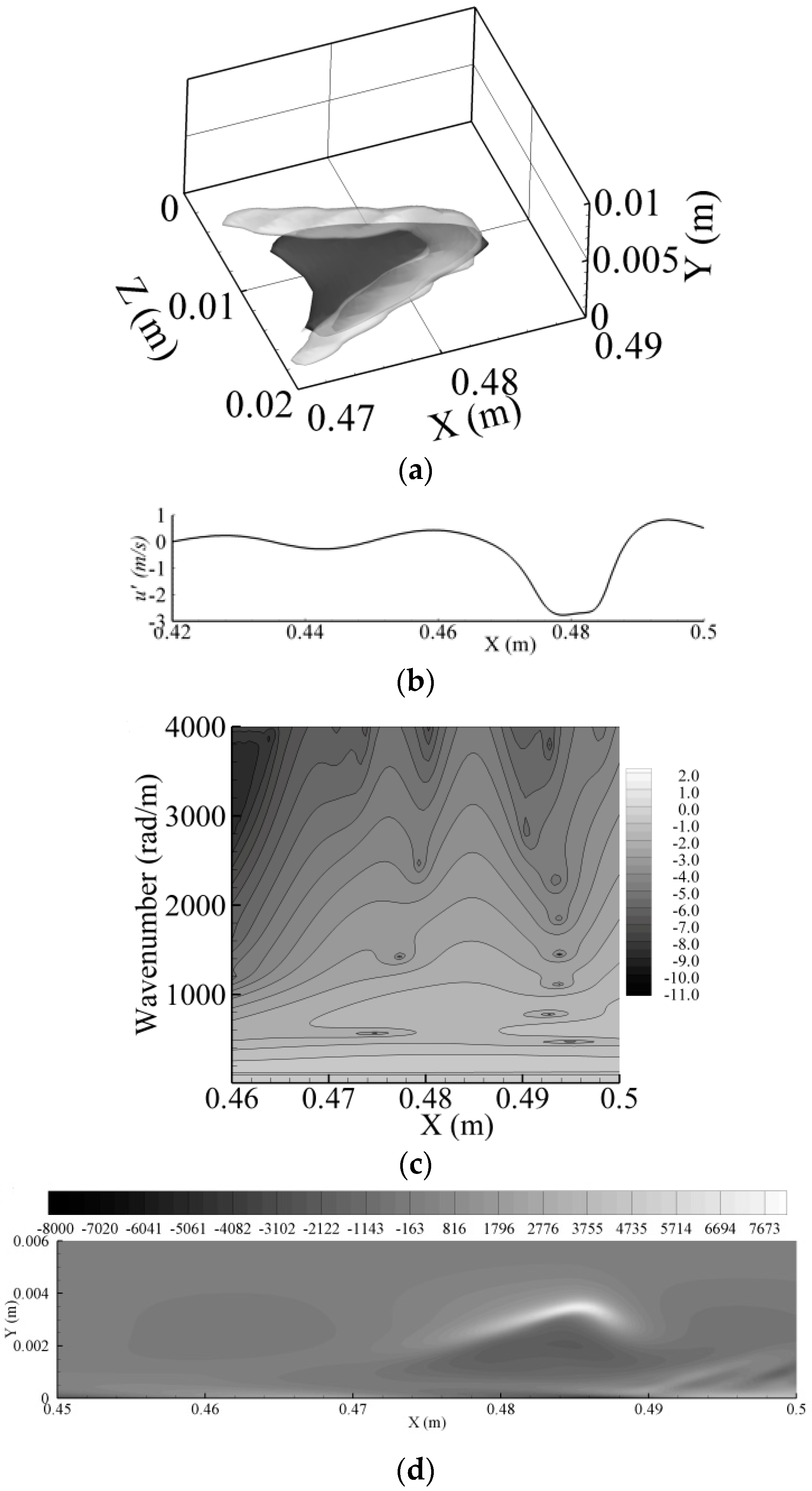
5.2. Λ-Vortex Evolution and First Spike Formation
After the primary Λ-vortex is formed, it continues to stretch, and its two legs become more slender as they propagate downstream. Figure 19 shows this development and the corresponding wavelet patterns. As shown in Figure 19a, the mature Λ-vortex has started to transform into an -vortex.
In Figure 19b, the spike starts to become blunt with one peak starting to separate into two. The two packets that are close enough to generate a sharp spike shown in Figure 18b start to separate. This spike formation is seen to arise from the interaction effects of the two wave packets when they are sufficiently close and have large enough energies. Figure 19c shows the twin-peak structure still present in the spectrum; but the two peaks spread to higher wavenumber, and their amplitude becomes stronger.
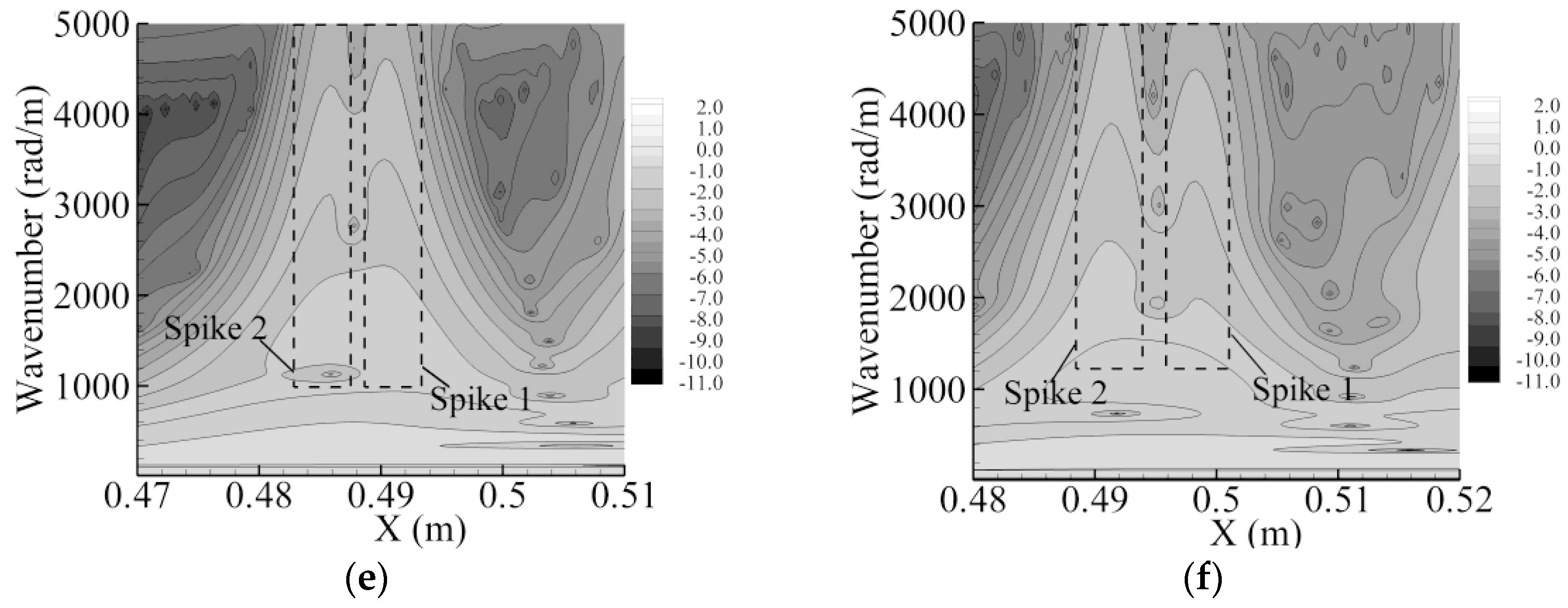
5.3. Formation of Ring-Like Vortex
Figure 20 shows the detachment process of the ring-like vortex from the remaining part of the Λ-vortex. Figure 20a shows that an -vortex has formed at = 0.066 s. The two legs of the -vortex are more slender than those of the Λ-vortex. At this stage, a ring-like vortex is about to form, and it tends to separate from the remaining of -vortex. The disturbance signal in Figure 20c shows the situation with two faint peaks seen. The wavelet transform results in Figure 20e are consistent with these observations with the two wavenumber peaks starting to separate. Here, it is noted that the energy at the highest wavenumbers though small is approaching the resolution of the numerical scheme, and accuracy beyond this stage may be affected.
Figure 20b at = 0.0675 s shows that the first ring-like vortex has separated from its mother vortex, and the two legs of the -vortex have reconnected with two thin links. At this stage, a second spike in the signal is formed (Figure 20d) resulting in two clear spikes, i.e., the second spike stage. The wavelet transform in Figure 20f shows a clear separation of the front and rear packets. It is seen that the front packet is essentially associated with the first ring-like vortex with the upper and lower wave packets first described in Borodulin and Kachanov’s experimental results [8,39] and which is seen clearly in physical space. Here, they are linked to the first and the second spike respectively. However, before their physical separation, these two distinct structures already exist in the primary Λ-vortex stage, which is revealed by the wavelet transform in Figure 18c.
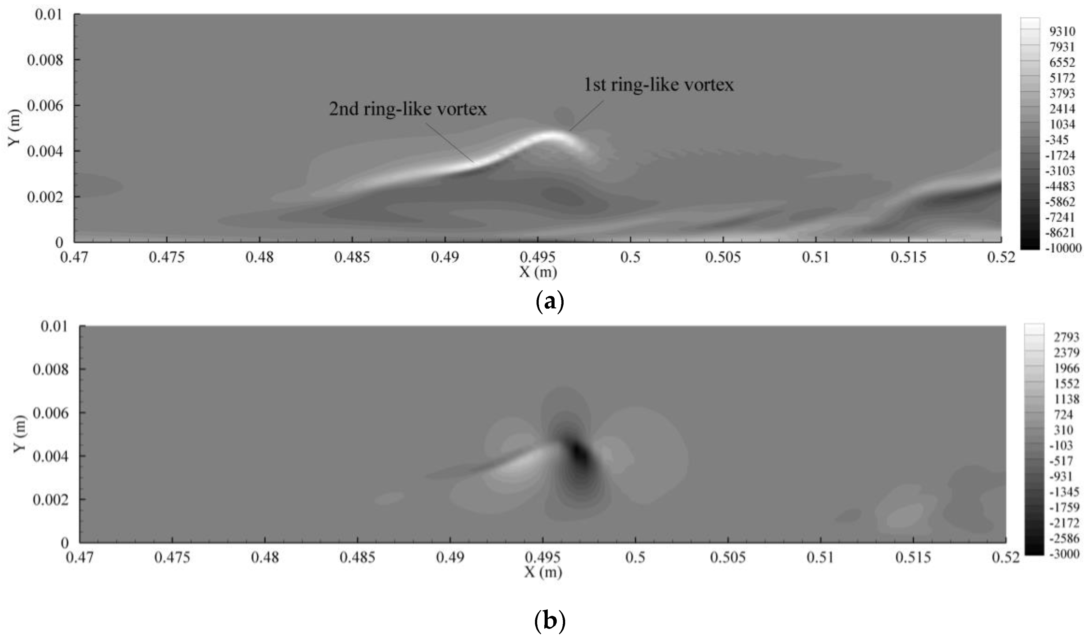
The pattern of the high shear layer is shown in Figure 21a. The first ring-like vortex forms at the head of Λ-vortex along with a hump being generated at the front of the high shear layer . It is seen that the tip of the pattern keeps growing strongly, which corresponds to the first ring-like vortex in Figure 20b. The tail part of the pattern corresponds to the second ring-like vortex. These patterns are similar to the ones reported for subharmonic resonance and fundamental resonance [10,16,19]. Contours of , the other part of spanwise disturbance vorticity , are shown in Figure 21b. Although the plot shows a similar “hook” shape in the streamwise direction as , its magnitude is only around 30% of , indicating the high shear is the main contributor to the spanwise disturbance vorticity up to the present stage.
Figure 21 also shows the stretching of the high shear layer. Though the two spike signals in Figure 20d have already separated, the high shear layer is still connected. The front high wavenumber component peak matches its tip at X = 0.498 m and the rear one at X = 0.492 m. As in the spike signal and the wavelet spectrum, the high shear layer tends to split into two parts (one goes with the first ring-like vortex and the other with the remaining Λ-vortex), therefore, combining the observations in Figure 20 and Figure 21, the high wavenumber components of the first ring-like vortex come from the “front peak” in the wavelet spectrum stemming from the one in Figure 18c, where the Λ-vortex is still in its primary stage. The “rear peak” in the wavelet spectrum in Figure 18c contributes to the continuing evolution of the remaining Λ-vortex. Further, both peaks are imbedded in the near wall high shear layer and in the spike region in the primary Λ-vortex stage.
6. Conclusions
A high order accuracy numerical model is used to simulate the experiments of [11] on an APG boundary layer transition induced by broadband disturbances. The numerical simulation results demonstrate that there may be common features in the boundary layer transition induced by small amplitude disturbances and particularly in the development of coherent structures. A wavelet analysis further shows that the local spectral components of the Λ-vortex and its associated high shear layer contain two wave packets during most of its life.
Due to the use of initial broadband disturbances in the simulations here, the coherent structures that arise in the transition process are distributed randomly both spatially and temporally. The coherent structures have different shapes, and most of them are asymmetric. However, they are qualitatively similar to those observed in the typical fundamental and subharmonic resonances. They all have a tip at their head and one or two legs at the rear.
Although the coherent structures exhibit different shapes and spatial distributions in the simulation of broadband disturbances, their spectrum are quite similar. They always contain a twin-peak structure, which forms prior to the maturity of the Λ-vortex. As the Λ-vortex evolves to the Ω-vortex and at a later stage when the first ring-like vortex forms, the two peaks of the high wavenumber components separate. The front one is related to the first spike or the first ring-like vortex and the rear one to the second spike or the other ring-like vortex. Thus, the results reveal the source location of high wavenumber disturbance in boundary layer transition flow: they are originally imbedded in the spike region and wall-region high shear layer and evolve with them.
Acknowledgments
The contributions of Jim C. Chen in this study are gratefully acknowledged.
Author Contributions
Weijia Chen designed and performed the numerical experiments; Weijia Chen and Edmond Y. Lo co-analyzed the data and co-wrote the paper.
Conflicts of Interest
The authors declare no conflict of interest.
References
- Cebeci, T.; Cousteix, J. Modeling and Computation of Boundary-Layer Flows: Laminar, Turbulent and Transitional Boundary Layers in Incompressible and Compressible Flows; Horizon Publishing: Long Beach, CA, USA, 2005. [Google Scholar]
- Schubauer, G.B.; Skramstad, H.K. Laminar-boundary-Layer Oscillations and Transition on a Flat Plate; National Bureau of Standards: Washington, DC, USA, 1948; pp. 251–292. [Google Scholar]
- Morkovin, M.V. On the many faces of transition. In Viscous Drag Reduction; Wells, C.S., Ed.; Plenum Press: New York, NY, USA, 1969; pp. 1–31. [Google Scholar]
- Kachanov, Y.S. On the resonant nature of the breakdown of a laminar boundary-layer. J. Fluid Mech. 1987, 184, 43–74. [Google Scholar] [CrossRef]
- Orszag, S.A.; Patera, A.T. Secondary instability of wall-bounded shear flows. J. Fluid Mech. 1983, 128, 347–385. [Google Scholar] [CrossRef]
- Klebanoff, P.S.; Tidstrom, K.D.; Sargent, L.M. The three-dimensional nature of boundary layer instability. J. Fluid Mech. 1962, 12, 1–34. [Google Scholar] [CrossRef]
- Kachanov, Y.S.; Kozlov, V.V.; Levchenko, V.Y. Nonlinear development of a wave in a boundary layer. Fluid Dyn. 1977, 12, 383–390. [Google Scholar] [CrossRef]
- Kachanov, Y.S. Physical mechanisms of laminar-boundary-layer transition. Annu. Rev. Fluid Mech. 1994, 26, 411–482. [Google Scholar] [CrossRef]
- Bake, S.; Fernholz, H.H.; Kachanov, Y.S. Resemblance of K- and N-regimes of boundary-layer transition at late stages. Eur. J. Mech. B-Fluids 2000, 19, 1–22. [Google Scholar] [CrossRef]
- Bake, S.; Meyer, D.G.W.; Rist, U. Turbulence mechanism in klebanoff transition: A quantitative comparison of experiment and direct numerical simulation. J. Fluid Mech. 2002, 459, 217–243. [Google Scholar] [CrossRef]
- Borodulin, V.I.; Kachanov, Y.S.; Roschektayev, A.P. Turbulence production in an APG-boundary-layer transition induced by randomized perturbations. J. Turbul. 2006, 7, 1–30. [Google Scholar] [CrossRef]
- Lee, C.B.; Li, R.Q. Dominant structure for turbulent production in a transitional boundary layer. J. Turbul. 2007, 8, 1–34. [Google Scholar] [CrossRef]
- Liu, C.; Lu, P. DNS study on physics of late boundary layer transition. In Proceedings of the 50th AIAA Aerospace Sciences Meeting, Nashville, TN, USA, 9–12 January 2012. [Google Scholar]
- Liu, C.; Yan, Y.; Lu, P. Physics of turbulence generation and sustenance in a boundary layer. Comput. Fluids 2014, 102, 353–384. [Google Scholar] [CrossRef]
- Chen, W.; Chen, J.C. Combined compact difference method for solving the incompressible navier-stokes equations. Int. J. Numer. Methods Fluids 2012, 68, 1234–1256. [Google Scholar] [CrossRef]
- Chen, W.; Chen, J.C.; Lo, E.Y. An interpolation based finite difference method on non-uniform grid for solving navier-stokes equations. Comput. Fluids 2014, 101, 273–290. [Google Scholar] [CrossRef]
- Fasel, H. Investigation of the stability of boundary layers by a finite-differencee model of the navier-stokes equations. J. Fluid Mech. 1976, 78, 355–383. [Google Scholar] [CrossRef]
- Fasel, H. Numerical investigation of the three-dimensional development in boundary-layer transition. AIAA J. 1990, 28, 29–37. [Google Scholar] [CrossRef]
- Rist, U.; Fasel, H. Direct numerical simulation of controlled transition in a flat-plate boundary layer. J. Fluid Mech. 1995, 298, 211–248. [Google Scholar] [CrossRef]
- Yeo, K.S.; Zhao, X.; Wang, Z.Y.; Ng, K.C. DNS of wavepacket evolution in a blasius boundary layer. J. Fluid Mech. 2010, 652, 333–372. [Google Scholar] [CrossRef]
- Chen, W. Numerical Simulation of Boundary Layer Transition by Combined Compact Difference Method. Ph.D. Thesis, Nanyang Technological University, Nanyang Ave, Singapore, 2013. [Google Scholar]
- Kachanov, Y.S.; Levchenko, V.Y. The resonant interaction of disturbances at laminar turbulent transition in a boundary-layer. J. Fluid Mech. 1984, 138, 209–247. [Google Scholar] [CrossRef]
- Borodulin, V.I.; Kachanov, Y.S.; Koptsev, D.B. Experimental study of resonant interactions of instability waves in a self-similar boundary layer with an adverse pressure gradient: I. Tuned resonances. J. Turbul. 2002, 3, 62. [Google Scholar] [CrossRef]
- Argoul, F.; Ameodo, A.; Grasseau, G.; Gagne, Y.; Hopfinger, E.; Frisch, U. Wavelet analysis of turbulence reveals the multifractal nature of the richardson cascade. Nature 1989, 338, 51–53. [Google Scholar] [CrossRef]
- Meitz, H.L. Numerical Investigation of Suction in a Transitional Flat-Plate Boundary Layer; The University of Arizona: Tucson, AZ, USA, 1996. [Google Scholar]
- Meitz, H.L.; Fasel, H.F. A compact-difference scheme for the navier–stokes equations in vorticity–velocity formulation. J. Comput. Phys. 2000, 157, 371–403. [Google Scholar] [CrossRef]
- Liu, C.H.; Maslowe, S.A. A numerical investigation of resonant interactions in adverse-pressure-gradient boundary layers. J. Fluid Mech. 1999, 378, 269–289. [Google Scholar] [CrossRef]
- Peyret, R. Spectral Methods for Incompressible Viscous Flow; Springer: Berlin, Germany, 2002. [Google Scholar]
- Hirsch, C. Numerical Computation of Internal and External Flows: Fundamentals of Computational Fluid Dynamics, 2nd ed.; Butterworth-Heinemann: Oxford, UK, 2007. [Google Scholar]
- Wu, X.H.; Moin, P. Direct numerical simulation of turbulence in a nominally zero-pressure-gradient flat-plate boundary layer. J. Fluid Mech. 2009, 630, 5–41. [Google Scholar] [CrossRef]
- Shaikh, F.N. Investigation of transition to turbulence using white-noise excitation and local analysis techniques. J. Fluid Mech. 1997, 348, 29–83. [Google Scholar] [CrossRef]
- Torrence, C.; Compo, G.P. A practical guide to wavelet analysis. Bull. Am. Meteorol. Soc. 1998, 79, 61–78. [Google Scholar] [CrossRef]
- Bertolotti, F.P.; Herbert, T.; Spalart, P.R. Linear and nonlinear stability of the blasius boundary-layer. J. Fluid Mech. 1992, 242, 441–474. [Google Scholar] [CrossRef]
- Hunt, J.C.R.; Wray, A.A.; Moin, P. Eddies, Stream, and Convergence Zones in Turbulent Flows. Available online: https://ntrs.nasa.gov/archive/nasa/casi.ntrs.nasa.gov/19890015184.pdf (accessed on 17 April 2017).
- Chakraborty, P.; Balachandar, S.; Adrian, R.J. On the relationships between local vortex identification schemes. J. Fluid Mech. 2005, 535, 189–214. [Google Scholar] [CrossRef]
- Ovchinnikov, V.; Choudhari, M.M.; Piomelli, U. Numerical simulations of boundary-layer bypass transition due to high-amplitude free-stream turbulence. J. Fluid Mech. 2008, 613, 135–169. [Google Scholar] [CrossRef]
- Jeong, J.; Hussain, F. On the identification of a vortex. J. Fluid Mech. 1995, 285, 69–94. [Google Scholar] [CrossRef]
- Borodulin, V.I.; Gaponenko, V.R.; Kachanov, Y.S.; Meyer, D.G.W.; Rist, U.; Lian, Q.X.; Lee, C.B. Late-stage transitional boundary-layer structures: Direct numerical simulation and experiment. Theor. Comput. Fluid Dyn. 2002, 15, 317–337. [Google Scholar] [CrossRef]
- Borodulin, V.I.; Kachanov, Y.S. Role of the mechanism of local secondary instability in K-breakdown of boundary layer. Soviet J. Appl. Phys. 1988, 3, 70–81. [Google Scholar]
Figure 1.
Comparison sketch of the investigation domain in streamwise direction between the experiments of [11] and the present simulation.
Figure 1.
Comparison sketch of the investigation domain in streamwise direction between the experiments of [11] and the present simulation.
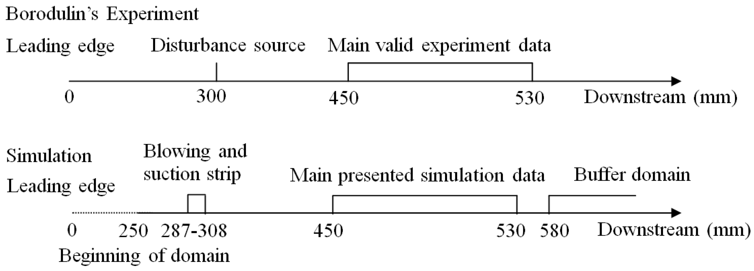
Figure 2.
Computational domain.

Figure 3.
Modified scaled wavenumber w1 and w2 plotted against scaled wavenumber w for the finite difference schemes on a non-uniform grid. (a) w1 for the first derivative. (b) w2 for the second derivative. CCD, Combined Compact Difference.
Figure 3.
Modified scaled wavenumber w1 and w2 plotted against scaled wavenumber w for the finite difference schemes on a non-uniform grid. (a) w1 for the first derivative. (b) w2 for the second derivative. CCD, Combined Compact Difference.

Figure 4.
The distribution of the two-dimensional disturbance source.
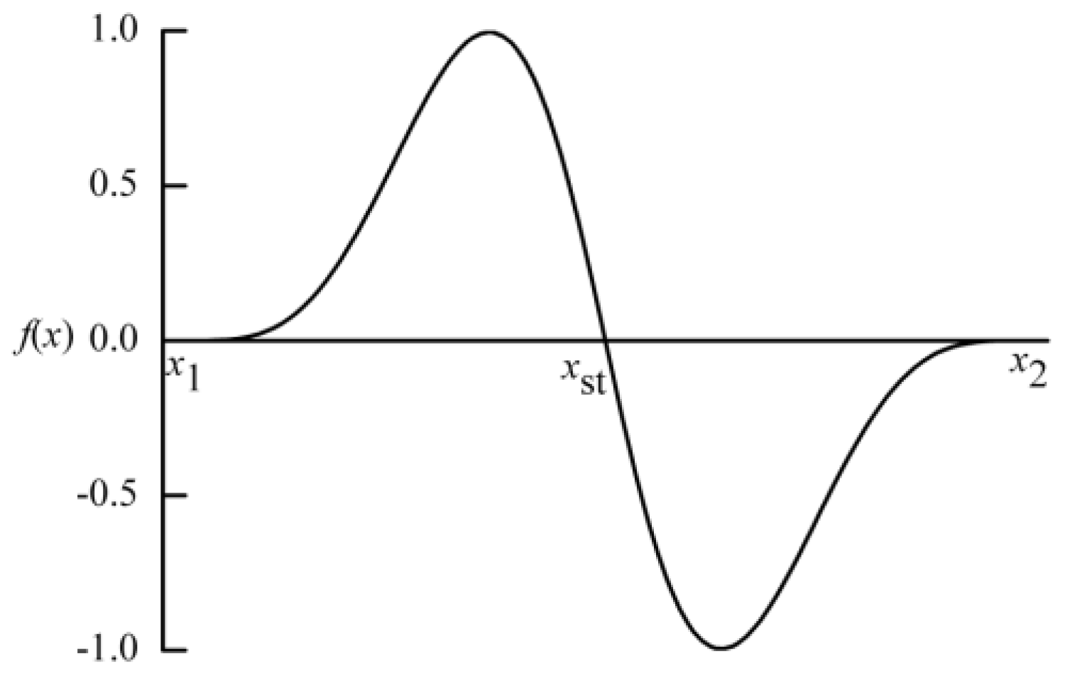
Figure 5.
Random signal in time space.
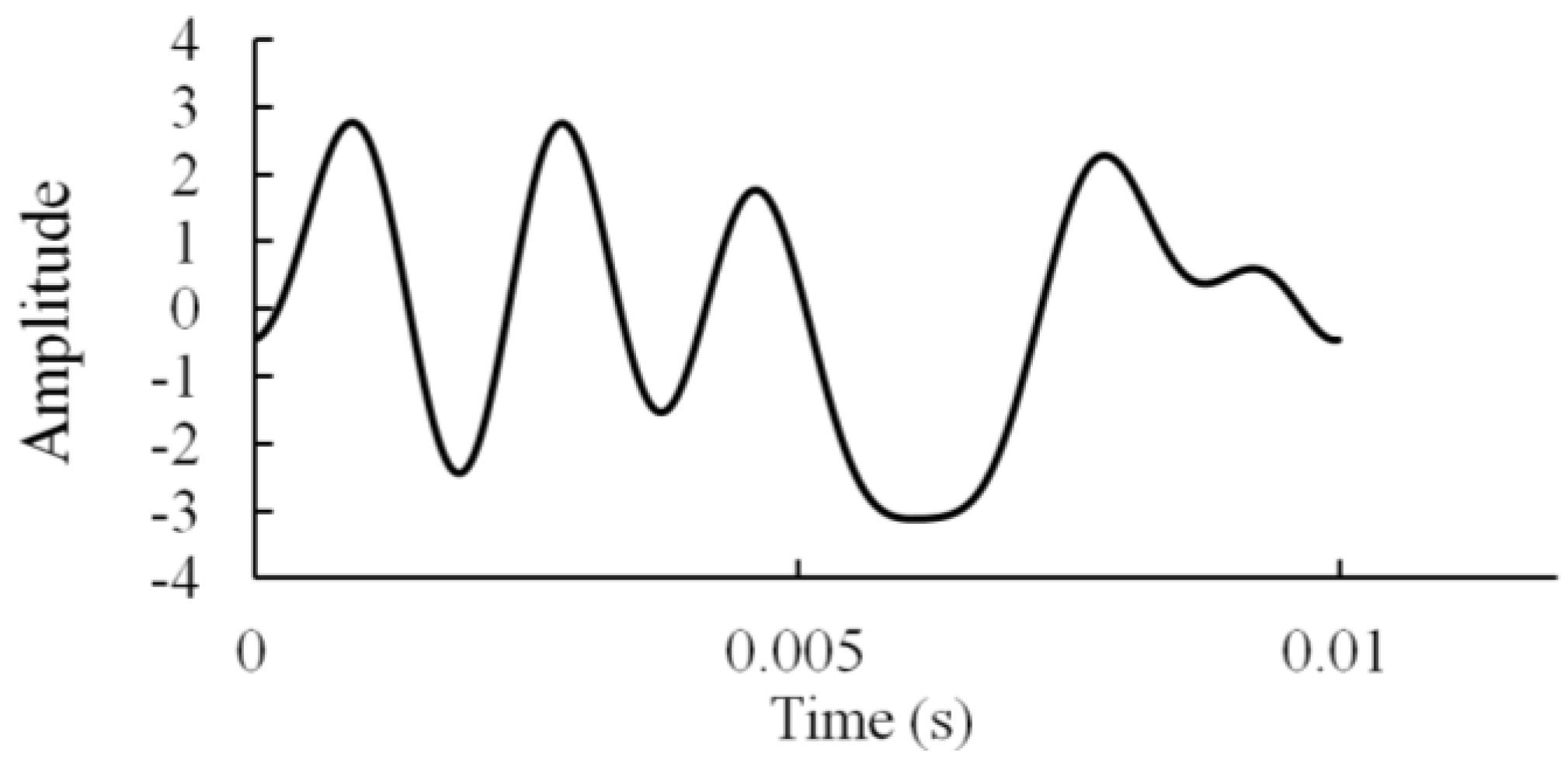
Figure 6.
Top hat frequency spectrum of the random signal . The vertical axis is the Fourier amplitude while the horizontal axis show frequency range up to 6 times the TS frequency of 109.1 Hz.
Figure 6.
Top hat frequency spectrum of the random signal . The vertical axis is the Fourier amplitude while the horizontal axis show frequency range up to 6 times the TS frequency of 109.1 Hz.

Figure 7.
Amplification of streamwise disturbance amplitude in resonant simulation. Left vertical axis: wave amplitude of subharmonic resonance with comparison of [23]. Right vertical axis: wave amplitude in 2D instability simulation with comparison of [33].

Figure 8.
Wall-normal profile of boundary layer disturbance amplitude at X = 450 mm and Z = 14 mm.

Figure 9.
Wave amplitude against frequency and spanwise Fourier modes at X = 450 mm and Y = 1 mm.

Figure 10.
Instantaneous contour of streamwise disturbance (m/s) at Y = 1.2 mm. (a) = 0.059 s; (b) = 0.072 s.
Figure 10.
Instantaneous contour of streamwise disturbance (m/s) at Y = 1.2 mm. (a) = 0.059 s; (b) = 0.072 s.


Figure 11.
Vortex visualization by Q-criterion at (a) = 0.066 s; (b) = 0.105 s.

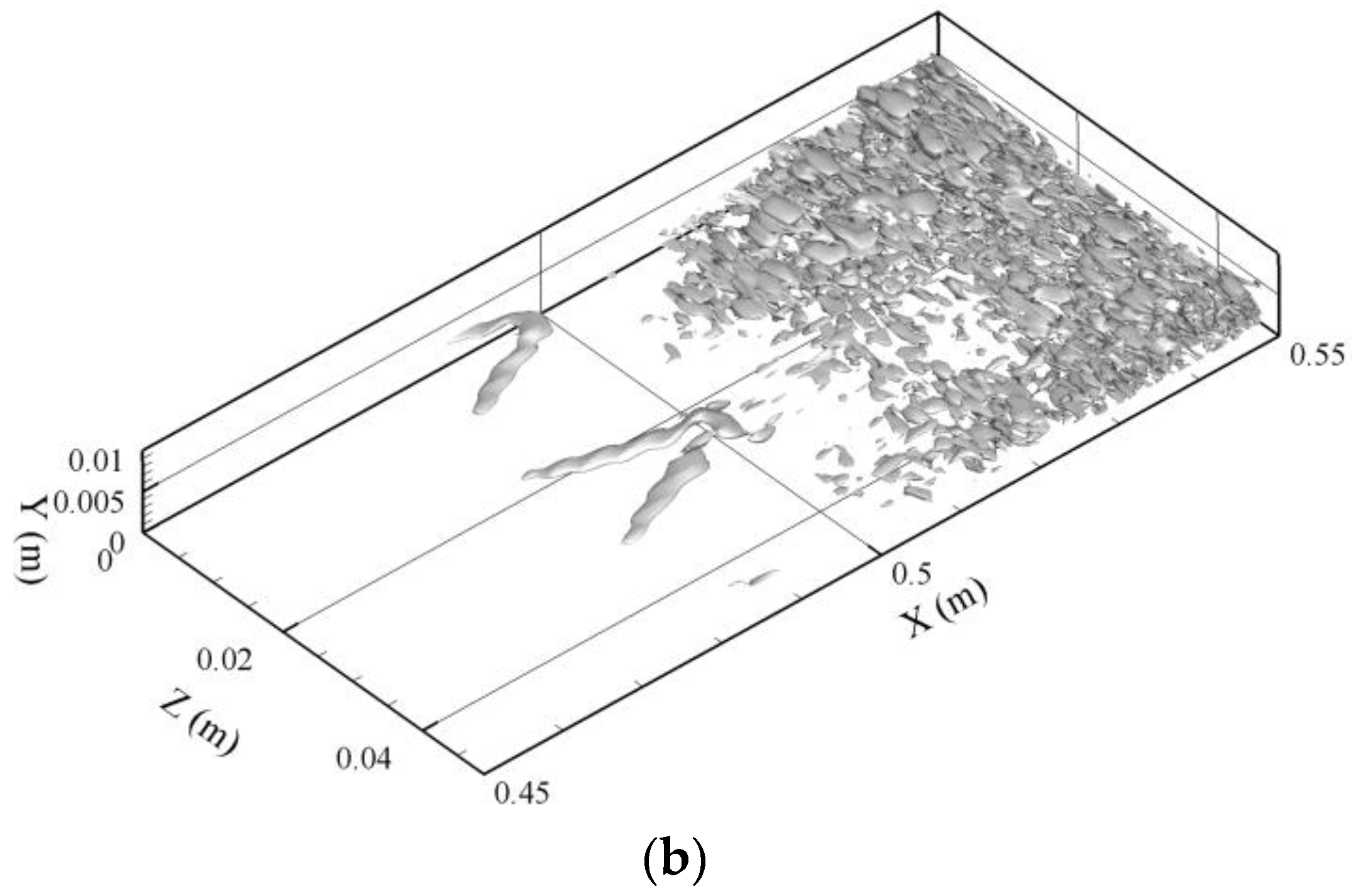
Figure 12.
Iso-surfaces of the streamwise disturbance velocities by plotting = −8%, at (a) = 0.053 s, (b) = 0.059 s, (c) = 0.067 s, (d) = 0.069 s.
Figure 12.
Iso-surfaces of the streamwise disturbance velocities by plotting = −8%, at (a) = 0.053 s, (b) = 0.059 s, (c) = 0.067 s, (d) = 0.069 s.

Figure 13.
Iso-surfaces of the streamwise disturbance velocities by plotting = −12%, at (a) = 0.059 s, (b) = 0.062 s, (c) = 0.067 s, (d) = 0.078 s.
Figure 13.
Iso-surfaces of the streamwise disturbance velocities by plotting = −12%, at (a) = 0.059 s, (b) = 0.062 s, (c) = 0.067 s, (d) = 0.078 s.
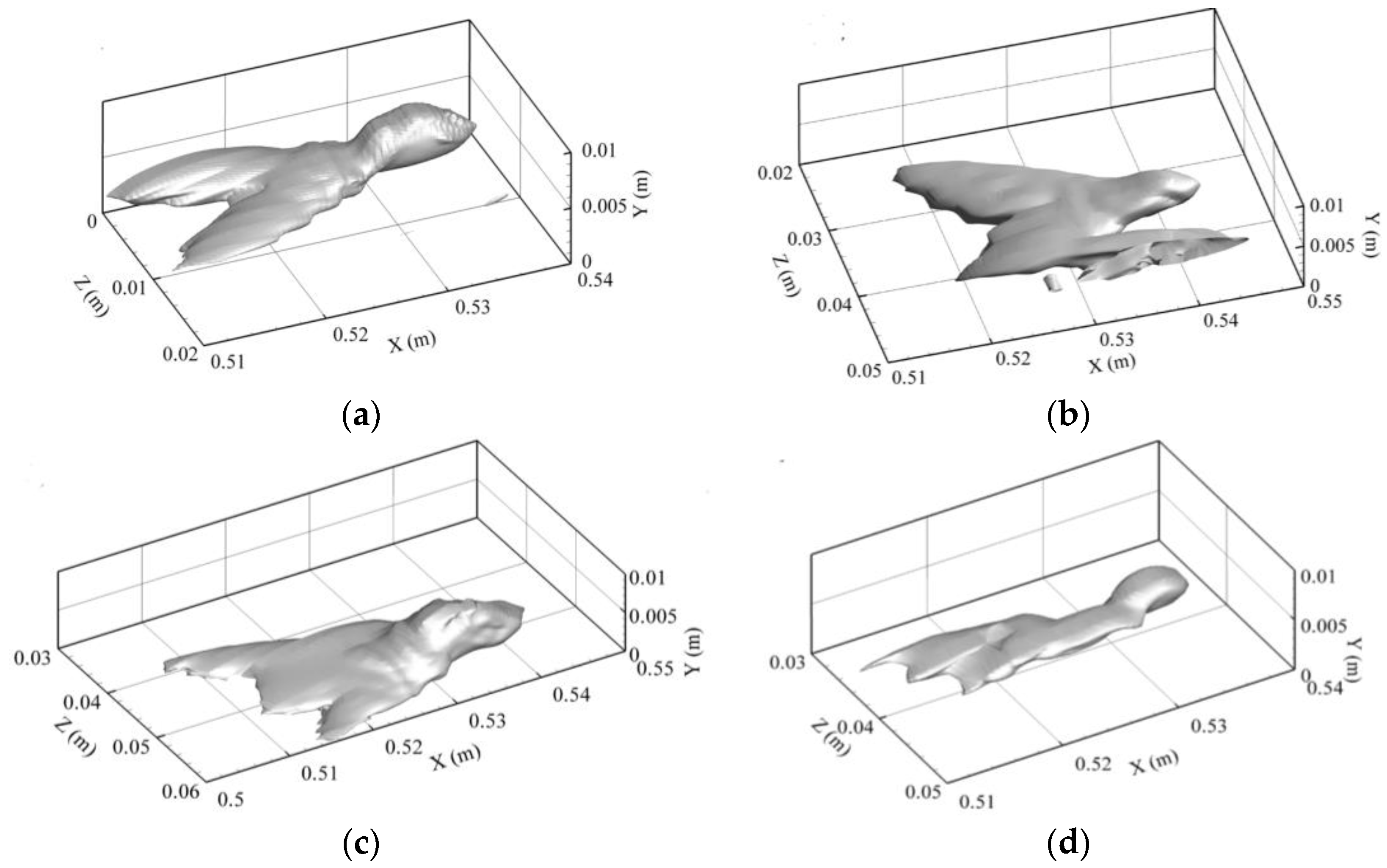
Figure 14.
Instantaneous contour of streamwise disturbance velocity (m/s) at Y = 1.18 mm and T = 0.056 s.
Figure 14.
Instantaneous contour of streamwise disturbance velocity (m/s) at Y = 1.18 mm and T = 0.056 s.
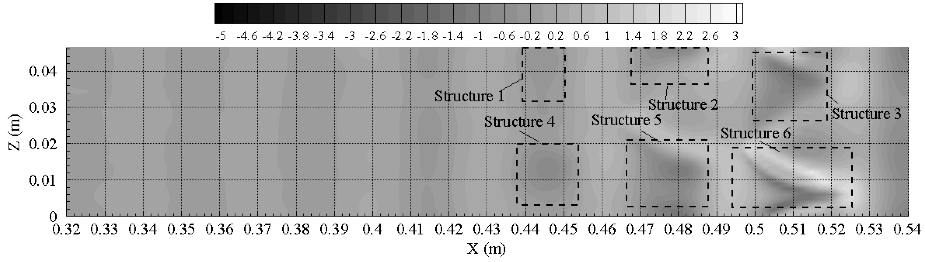
Figure 15.
Vortex visualization by Q-criterion at T = 0.056 s.
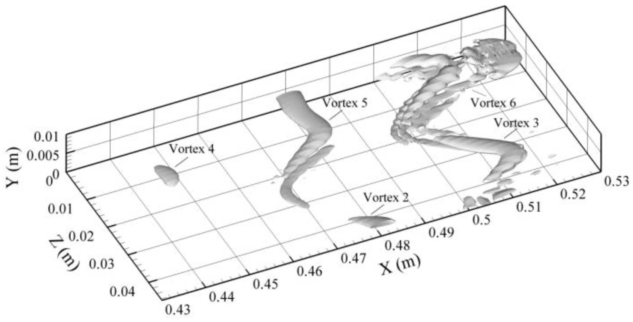
Figure 16.
Continuous Wavelet Transform (CWT) results at T = 0.056 s, Y = 1.18 mm, Z = 13.5 mm, (a) streamwise disturbance signal and (b) wavelet transform of the streamwise disturbance velocity (log10 (m/s)).
Figure 16.
Continuous Wavelet Transform (CWT) results at T = 0.056 s, Y = 1.18 mm, Z = 13.5 mm, (a) streamwise disturbance signal and (b) wavelet transform of the streamwise disturbance velocity (log10 (m/s)).
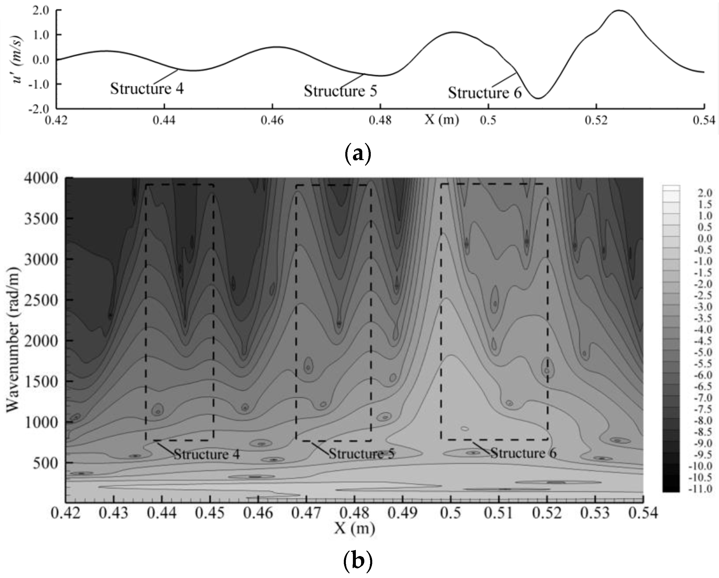
Figure 17.
Computed evolution of (1/s) at Z = 0.0135 m, T = 0.059 s.

Figure 18.
(a) Visualized evolution of rhombus-like structure (dark gray) by = −0.4 m/s (57% of local minimum) and primary vortex (transparent light gray) by the Q-criterion. (b) Streamwise disturbance at = 0.0135 m, Y = 1.4 mm. (c) Wavelet transform of the streamwise disturbance velocity (log10 (m/s)) at Z = 0.0135 m, Y = 0.0014 m. (d) contours at Z = 0.0135 m. (a) to (d) are plotted at T = 0.053 s.

Figure 19.
(a) Evolution of the spike region (dark gray) with = −1.5 m/s (60% of local minimum) and a Λ-vortex (transparent light gray) according to the Q-criterion. (b) Corresponding streamwise disturbance velocity at Z = 0.0135 m, Y = 2 mm. (c) Wavelet transform of the streamwise disturbance velocity (log10 (m/s)) at Z = 0.0135 m, Y = 2 mm. (d) at Z = 0.0135 m. (a) to (d) are plotted at T = 0.0649 s.

Figure 20.
Evolution of the spike region (dark gray) with = −4.0 m/s (66% of local minimum) and a Λ-vortex (transparent light gray) according to the Q-criterion at (a) T = 0.066 s, (b) T = 0.0675 s. Corresponding streamwise disturbance velocity at Z = 0.0135 m, Y = 3.12 mm and (c) T = 0.066 s; (d) T = 0.0675 s. Wavelet transform of the streamwise disturbance velocity (log10 (m/s)) at Z = 0.0135 m, Y = 3.12 mm and (e) T = 0.066 s; (f) T = 0.0675 s.
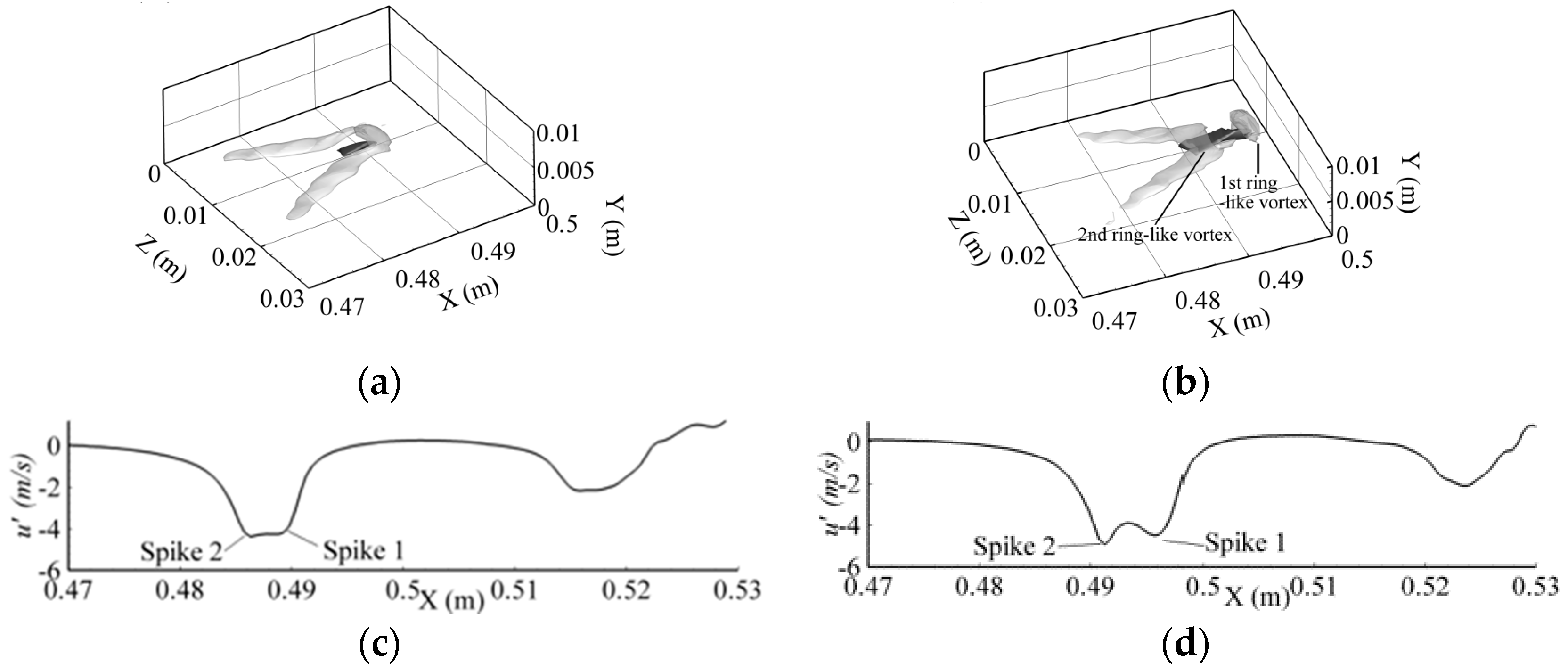

Figure 21.
(a) High shear layer (1/s), (b) (1/s) at Z = 0.0135 m, T = 0.0675 s.


Table 1.
Parameters of flow and computational domain. TS, Tollmien–Schlichting.
| Streamwise Grid Points | 1200 | ΔX Interval Per TS Wave Length | 61 |
|---|---|---|---|
| ΔX (mm) | 5 | Wall-normal grid points | 120 |
| ΔYmax (mm) | 0.01 | Spanwise grid points | 32 |
| Spanwise modes | 16 | ΔZ (mm) | 1.4 |
| ΔT (s) | 6.56 × 10⁻⁶ | ΔT interval per TS wave period | 1400 |
| TS wave frequency (Hz) | 109.1 | TS wave number (rad/m) | 205.9 |
© 2017 by the authors. Licensee MDPI, Basel, Switzerland. This article is an open access article distributed under the terms and conditions of the Creative Commons Attribution (CC BY) license (http://creativecommons.org/licenses/by/4.0/).
Share and Cite
MDPI and ACS Style
Chen, W.; Lo, E.Y. High Wavenumber Coherent Structures in Low Re APG-Boundary-Layer Transition Flow—A Numerical Study. Fluids 2017, 2, 21. https://doi.org/10.3390/fluids2020021
AMA Style
Chen W, Lo EY. High Wavenumber Coherent Structures in Low Re APG-Boundary-Layer Transition Flow—A Numerical Study. Fluids. 2017; 2(2):21. https://doi.org/10.3390/fluids2020021
Chicago/Turabian StyleChen, Weijia, and Edmond Y. Lo. 2017. "High Wavenumber Coherent Structures in Low Re APG-Boundary-Layer Transition Flow—A Numerical Study" Fluids 2, no. 2: 21. https://doi.org/10.3390/fluids2020021