
Hydrodynamics and Oxygen Bubble Characterization of Catalytic Cells Used in Artificial Photosynthesis by Means of CFD


1
Catalonia Institute for Energy Research (IREC), Marcel·lí Domingo 2, 43007 Tarragona, Catalonia, Spain
2
Department of Applied Science and Technology (DISAT), Politecnico di Torino, Corso Duca degli Abruzzi 29, 10129 Torino, Italy
3
Chemical Engineering Department, Universitat Rovira i Virgili, Av. Països Catalans 26, 43007 Tarragona, Catalonia, Spain
*
Authors to whom correspondence should be addressed.
Fluids 2017, 2(2), 25; https://doi.org/10.3390/fluids2020025
Submission received: 21 February 2017
/
Revised: 11 May 2017
/
Accepted: 12 May 2017
/
Published: 16 May 2017
(This article belongs to the Special Issue Advances in Hydrodynamics)
Abstract
:Miniaturized cells can be used in photo-electrochemistry to perform water splitting. The geometry, process variables and removal of oxygen bubbles in these cells need to be optimized. Bubbles tend to remain attached to the catalytic surface, thus blocking the reaction, and they therefore need to be dragged out of the cell. Computational Fluid Dynamics simulations have been carried out to assess the design of miniaturized cells and their results have been compared with experimental results. It has been found that low liquid inlet velocities (~0.1 m/s) favor the homogeneous distribution of the flow. Moderate velocities (0.5–1 m/s) favor preferred paths. High velocities (~2 m/s) lead to turbulent behavior of the flow, but avoid bubble coalescence and help to drag the bubbles. Gravity has a limited effect at this velocity. Finally, channeled cells have also been analyzed and they allow a good flow distribution, but part of the catalytic area could be lost. The here presented results can be used as guidelines for the optimum design of photocatalytic cells for the water splitting reaction for the production of solar fuels, such as H2 or other CO2 reduction products (i.e., CO, CH4, among others).
1. Introduction
The production and storage of energy obtained from renewable sources, the reduction of CO2 emissions into the atmosphere and its re-use are currently some of the main challenges for mankind. Artificial photosynthesis has been used in attempts to mimic the natural water splitting process and to use of the sunlight as an energy source to produce molecules that can be used as feedstock and for energy storage [1,2]. Therefore, efforts to develop renewable, carbon-neutral fuel sources have led to a new research and development focus on sunlight-driven water-splitting systems [3]. Among these systems, photo-electrochemical (PEC) water splitting devices are used to exploit renewable sources, i.e., water and sunlight, to produce O2 and H2. Moreover, the generated hydrogen can also be used to reduce CO2 for the production of either other C-containing fuels or high added-value chemicals (i.e., CO in syngas, CH4, methanol and ethanol among others) [4].
Many studies have been conducted with the aim of increasing the solar-to-hydrogen (STH) or solar-to-fuel (STF) conversion efficiencies of PEC devices [5,6,7]. Most of them have been focused on improving the design of photo-electrocatalysts (semiconductors such as TiO2 and ZnO, BiVO4, Fe2O3, WO3, Cu2O/CuO) [8,9,10] and catalysts (i.e., Pt, or Ir, Ru, Co or Mn oxides, etc.) [11]; on the electrode structure modification (from the nano- to micro-scopic level) [12,13], on changes in the operative conditions (i.e., pressure, temperature, kind of electrolyte and ion concentrations ) [14,15] and on the development of different cell configurations (i.e., with a single photo-electrode, tandem photosystems with a Z scheme, photovoltaic (PV)-PEC photosystems and buried PV photo-systems without photo-electrodes) [5,6].
As far as PEC reactors are concerned, two-compartment PEC cells are generally preferred, from both the cost and safety viewpoints. In such a system, the O2, produced through water oxidation at the anode, is separated directly from the reduction products (i.e., H2, CO, etc.) that form at the cathode, due to the presence of a proton exchange membrane (PEM), which is used for both H+ transport and to separate the anodic and cathodic chambers. The housing of such a reactor should have a transparent window, to allow sunlight irradiation, and current collectors, which can either be integrated with the electrodes or not. The overall cell potential of the electrolysis cells that has to be applied to a PEC electrolyzer can be calculated as the sum of: the minimum thermodynamic potential required for the total cell reaction (E°: Nernst potential); the kinetic overpotentials associated with the anodic and cathodic reactions at the catalyst surfaces (i.e., ηOx, for O2 evolution and ηRed for H2 evolution or for the formation of other desired CO2-reduction products, such as syngas [16]); the concentration overpotential (ηconc) and the ohmic resistance losses (ηohm), which depends on both the electrical contacts and the conductivity of the electrocatalyst substrates) [3,17]. ηOx, ηRed and ηohm depend on the electrode materials and electron transport, but ηconc, which is governed by the proton transport in the electrolyte, has been investigated less than the former ones.
Proton conduction is often more critical than electron conduction, since high ionic conductivity is difficult to achieve [5]. Unlike polymeric exchange membrane (PEM) electrolyzers, in which the catalysts are closely coupled to the PEM forming membrane-electrode-assemblies (MEA), the liquid and PEM electrolytes in most PEC devices are both media for H+ transport. In fact, there are few examples of transparent, conductive and porous electrode supports that can be used to form MEA in PEM photo-electrolyzes. However, in a recent work [12], thin transparent quartz sheets, covered by fluorine-doped tin oxide (FTO), were laser-drilled and used as supports of both TiO2 and Pt nanoparticles, thus constituting electrodes that were sandwiched with a Nafion membrane to form a transparent MEA for water splitting and H2 production. In other works, photocatalysts and catalysts (e.g., TiO2 and Pt powders) have been embedded with a suitable amount of conductive carbon black powder in Nafion membranes to form a MEA for H2 production [18]. Therefore, since liquid electrolytes generally have a lower level of conductivity than solid ones; the distance and the pathway for proton transport between electrode surfaces are important aspects in the design of PEC cells. Nocera and co-workers [19] obtained a 2.5% STF conversion efficiency using a monolithic and wireless H2 production device, in which protons generated at the front of the cell had to move around the electrode to reach the back, while a 4.7% STF conversion efficiency was obtained by employing a wired PEC system with facing electrodes and a shorter proton transport distance.
Microfluidic flow cells (MFCs) are suitable for use as PEM photo-electrolyzers and can be designed to minimize dead volumes and optimize retention times. MFCs have been demonstrated, in several experimental studies, to be effective reactors and versatile analytical tools for water splitting for H2 production [12,20] and for the electro-reduction of CO2 [16,21]. However, not much modelling work has been reported in the literature on such systems, although the electrolyte distribution at the device inlets and the fluid dynamics of the liquid electrolyte inside the electrode chambers both have a great influence on ηconc and on the performance of a PEC device. On one hand, they need to be optimized in order to guarantee interaction between the reactants (i.e., water, CO2) and the catalytic surfaces. On the other hand, the bubbles of gaseous products (i.e., O2, H2, CO, etc.), which tend to remain attached to the electrocatalyst surface, need to be removed, in order to avoid a reduction in the reaction rate, due to a decrease in the effective active area and in the reactant concentration [22]. Moreover, the influence of the solar incident flux on the flow field and temperature distribution can also have an effect on the (photo) catalyst efficiency, reaction rates and on the final PEC reactor performance. In some recent works, theoretical models have been developed to analyze the formation and accumulation of bubbles on BiVO4 porous photocatalyst and Pt catalyst surfaces, and their influence on the photoelectric response (as a consequence of the O2 and H2 production rates) for different applied potentials under dark and light conditions [22,23]. In one of these models, which employs a percolation approach, it was shown that the photocurrent density decreases over the time due to bubbles generation, under static flow conditions at a fixed applied bias [22]. It was also found that if the applied bias is raised, the current density increases proportionally, and as a result, a larger concentration of molecular oxygen covers the anodic electrode surface with bubbles in a shorter time. However, under light conditions, the critical value of the electrode coverage factor (βc) increased for higher bias potentials [22]. In the other model, the formation of bubbles has been modeled by using a kinetic equation at the interface, considering the adsorption mechanism, where the adsorption term, hypothesized to be proportional to the current density, describes the formation of the bubbles on the electrode, whereas the desorbing term takes into account the detachment of the bubbles from the electrode [23]. Qureshi et al. [21] performed numerical simulations of a two-chamber PEC reactor, in which both transport phenomena (i.e., Navier-Stokes equation), and an energy equation for the electrolyte and radiative transfer equation were included, and they found that both the H2 production rate and STH efficiency were enhanced by increasing the solar incident flux from 500 to 2000 W/m2, considering an Fe2O3 photoanode and a Pt cathode as a case study. Wu et al. [21] presented a steady-state isothermal model for the electrochemical reduction of CO2 to CO in a microfluidic flow cell, which integrates charge, mass, and momentum transport with electrochemistry for both the cathode and anode, in order to determine the kinetic parameters at different flow rates while varying the applied cell potentials.
Nevertheless, simulations from a macroscopic point of view focused on the optimization of the design of PEC devices have not been developed. CFD is a useful computing tool that uses numerical analysis to solve and investigate problems that involve fluid flows [24,25,26]. It simulates the interaction of liquids and gases with surfaces defined by boundary conditions [27]. This method has already been used to simulate photo-electrochemical reactors for hydrogen production [28], and other types of fuel cells, such as solid oxide [29] or redox cells [30]. Multiphase problems can also be dealt with in CFD simulations, and they allow bubbles inside a liquid medium to be simulated [31]. In this study, CFD simulations have been carried out to assess the most efficient design of a microfluidic PEC cell.
2. Methodology
2.1. Simulations and Governing Equations
All the models were sketched with the commercial ANSYS Design Modeler 14 software. The grid was designed using ANSYS Mesh 14. All the CFD simulations were carried out using ANSYS Fluent 14. A Dell Precision T7500 Workstation was used with one Xeon E5530 processor core (due to license constraints) and 16 MB RAM.
In this work, a mathematical model composed by a set of conservation laws for mass (1) and momentum (2) was used by ANSYS Fluent:
where ρ is the density, p is the static pressure, t is time, is the velocity vector, μ is the molecular viscosity, ρ is the gravitational force and is the external body force.
Because of the velocities used in the experiments and the corresponding Re numbers (indicated below), regime was laminar in all cases. Therefore, no turbulence model was used.
To simulate multiphase (liquid-gas), the Explicit Volume of Fluid (VOF) model was used. The explicit VOF model is used to model immiscible fluids including liquid-gas case with clearly defined interface. The explicit scheme is appropriate when surface tension is important (which applies in this case) and allows using Geo-Reconstruct discretization in the simulation, which has the advantage to avoid numerical diffusion and allow high accuracy curvatures.
VOF model solves a single momentum equation throughout the domain (Equation (2)) and the resulting velocity field is shared among the phases. The properties used in the transport Equations (1) and (2) are determined by the presence of the component phases in each control volume. In this case, where a two-phase system exists, the density in each cell is given by:
where α is the volume fraction and the subscripts 1 and 2 represent the two components, as .
The tracking of the interface between the two phases existing in this application is accomplished by the solution of a continuity equation for the volume fraction of one of the phases. For the explicit approach, the standard finite-difference interpolation is applied to the volume fraction values computed at the previous time step. Therefore, the continuity equation used for the q phase is as follows:
where n + 1 is the index for the current time step (so n is the index for the previous one), p and q are phase indexes, f is the index for the current face, V is the volume of the cell, U is the volume flux based on the normal velocity and is the mass transfer from the indicated phases.
These schemes require transient time modelling and to have a global Courant number lower than an appropriate value (2 in this case). Courant number is computed according to Equation (5). It depends on the characteristic velocity (m/s), characteristic grid size (m) and time step (s). Because of the two first values imposed in this case, the time step needs to be around 5 × 10⁻⁶ s.
The explicit VOF model allows including the effects of surface tension and wall adhesion. Both models used in Fluent are those proposed by Brackbill [32].
Regarding the surface tension, the model considers that the pressure drop across a surface (Δp) depends on a surface tension coefficient and a surface curvature as measured by two radii in orthogonal directions (R):
σ is the surface tension coefficient, which in this case where water corresponded to the continuous phase and oxygen to the disperse phase, the value used was 0.07286 N/m [33].
In the results section, the mean values of different parameters, such as velocity, as well as the standard deviations are presented in the results section. The mean values of a plane or a volume have been obtained by calculating the mean value of all the PEC cell parameters that are affected. The standard deviation makes it possible to know how similar the values of a property within the PEC cells are with respect to the mean value.
2.1.1. Hydrodynamic Study
All the used models were 3D models. Grid Independence Tests (GIT) were performed to ensure that the simulation results were not influenced by the mesh. The final configuration consisted of a structured grid with 731.373 hexahedral elements. Simulations were carried out considering water as the fluid in the laminar regime, because of the considered velocities and geometrical parameters. The models considered only half of the geometry, and a symmetry boundary was used for the side that represented the interface between the other half of the model. The other boundary conditions that were considered were: inlet velocity, outflow and walls.
Several types of modules were simulated (Figure 1).
The reference module (geometry A) is the PEC cell that was employed in the experimental part. This geometry corresponds to a standard PEC cell configuration for this type of application, and it consists of a rectangular cavity where the top glass wall includes the catalyst and the side of the membrane from which the protons exit. Before the central rectangular cavity is reached, some distributors are positioned to help the liquid disperse through the whole cavity. From this initial design, other models were simulated with variations from the reference module to check the hydrodynamic performance. The variations included: introducing channels into the central cavity (geometry B), changing the cell depth and changing the configuration of the distributors with respect to geometry A.
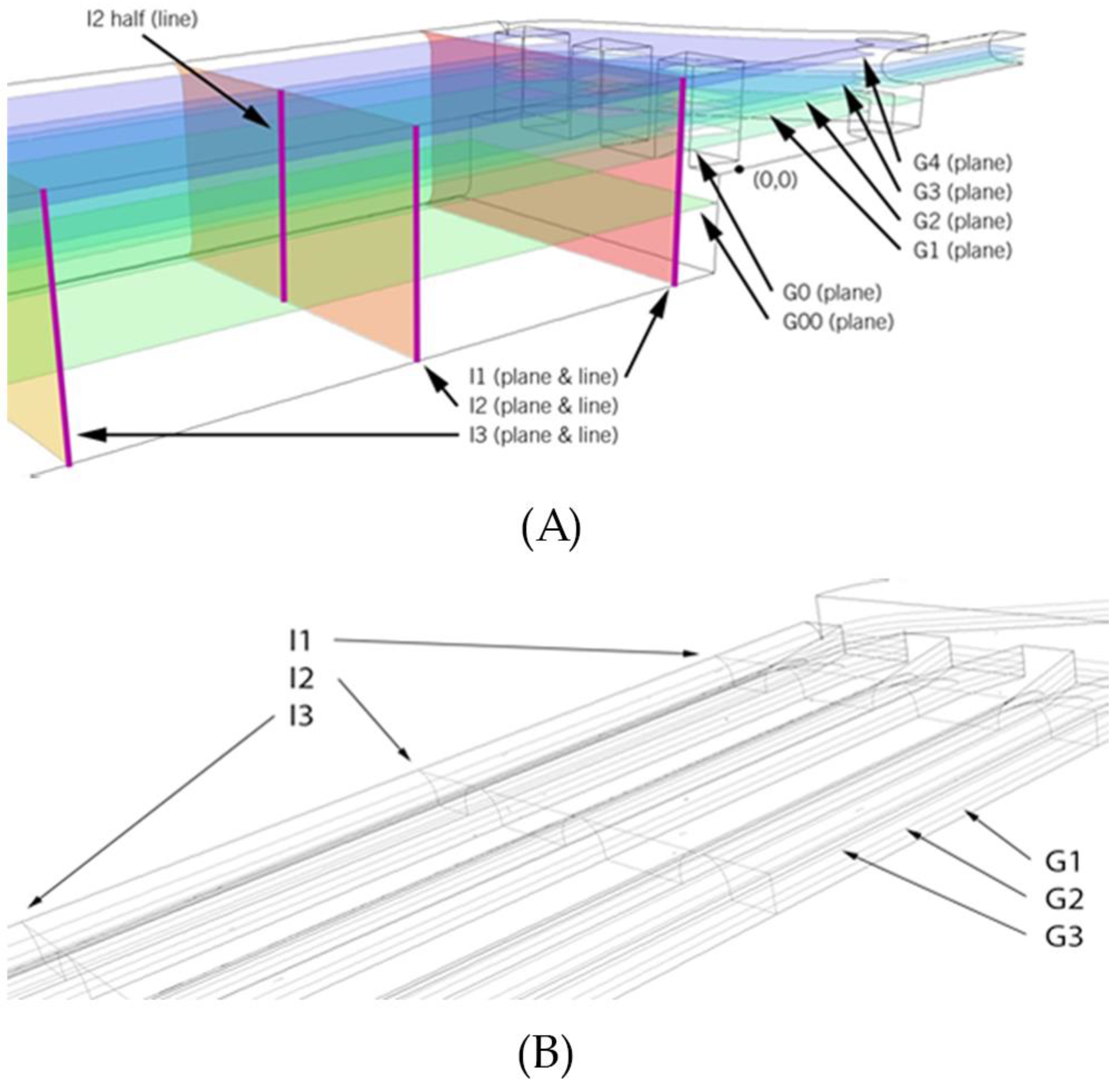
In order to evaluate the results, various properties were computed and compared at several planes and edges in the geometry. Figure 2 identifies the planes and edges that the results refer to. These planes and edges are located midway between the volume boundaries and the plane limits, respectively.
These simulations considered some simplifications: laminar flow, no reactions, no use of other special models, User Defined Functions or 3D simulations. Grid Independence Tests (GIT) were also performed as explained in Section 2.1.1.
2.1.2. Bubble Characterization
In order to assess the removal of oxygen bubbles from the cell, oxygen generation needs to be included in the simulations. As no kinetic data were available, a model developed in a previous work, which considers oxygen generation [19], was used. This model offered the advantage of allowing the case to being less complex than having to simulate the reaction (only a multiphase was introduced). Several oxygen inlet velocities were considered to perform sensitivity analysis and to obtain generalized results.
ANSYS Fluent includes special models to simulate porous surfaces. Some preliminary simulations were conducted to check the correspondence between the results obtained using these models and videos recorded during the experiments. As the simulation results did not show agreement with the experimental ones, the strategy was discarded. The alternative approach of considering orifices on the surface as oxygen velocity inlets instead showed a good correspondence with the experimental results, and this strategy was therefore adopted for the other tests.
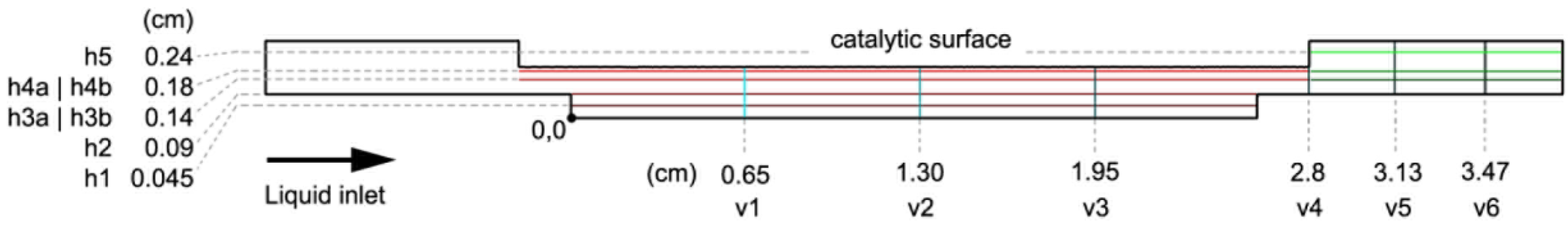
The simulations were carried out in 2D, because of computing requirements. One 3D simulation was also performed for validating purposes. The 2D models were on a transversal central plane, as shown in Figure 3. This figure also indicates the control lines established for a post-result analysis, which are located midway between the plane limits. The used boundary conditions were: velocity inlet for the liquid and gas inlet edges, pressure outlet for the outlet edge and walls for the defined edges. In order to have enough resolution to resolve the bubble contours, the grid elements had a minimum side length of 0.025 mm; 3 levels of refinement were applied to the catalytic boundary and 2 levels to the oxygen wet walls. The model consisted of 12,954 elements with these conditions, almost all of which were rectangular.
The 3D simulation was performed by projecting the 2D geometry until a thickness of 0.46 mm was reached. The grid dimensions were balanced to obtain enough resolution at the oxygen inlets and an acceptable number of elements (206,663). No refinements were introduced. The boundary conditions were the same as those of the 2D cases, except for the lateral faces, which were set to symmetry boundary conditions. The 3D simulation allows the behavior of bubbles to be envisioned when the third dimension is considered.
One of the limitations of performing 2D simulations is that there is not a correct match between the liquid inlet velocity and mean liquid velocity inside the cell. In 3D simulations, the cross-section differs to a great extent from the inlet to the central area. As the flow rate is constant, the velocity differs as a function of the cross-section. This can be realized by comparing the Re numbers. At 1 m/s, while Re at the inlet is 2077, it is 139 at the central cavity. In order to take into account this deviation, Table 1 shows the computed equivalences for each liquid inlet velocity for the 2D and 3D simulations.
The simulations and results were expressed using the following nomenclature: L#G#XX, where the number after L represents the liquid inlet velocity (m/s), the number after G represents the gas inlet velocity (m/s) and the last two characters are the gravity direction. GC refers to the same direction as the gas inlet, GF refers to the opposite direction from the gas inlet and GM refers to the gas direction contrary to the liquid inlet direction.
Table 2 summarizes the meshes used in the simulations and their main properties.
2.2. Photo-Electrochemical Tests
Photo-electrochemical tests were carried out with the geometry described in Figure 3 to validate some simulation results. The validation consisted of recording videos for certain experiments and comparing them with the simulated results.
The experimental photoelectrochemical characterizations were performed with BiVO4 photoanodes that were prepared as reported in [22], and were carried out in a 0.1 M NaPi buffer (pH~7), using a two-electrode configuration (BiVO4 electrode and a sputtered platinum rod both deposited on FTO-glass substrates). Back-illumination of the BiVO4 working electrode was employed, since higher IPCE spectra have been reported under such conditions than when front- illumination is used [34]. Chrono-amperometry (CA) measurements were performed at 0.6 V vs. Ag/AgCl under continuous visible light irradiation, using a LUXIM (LIFI-STA-40-01) lamp. The intensity of the light was maintained at 100 mW cm−2 by adjusting the distance between the source and the PEC.
The images obtained from the videos were analyzed with ImageJ software to assess the bubble concentration and size distribution [35].
3. Results and Discussion
3.1. Hydrodynamics Inside the Photoelectrochemical Cells
The purpose of this study was to establish which hydrodynamic conditions favor a homogeneous liquid distribution inside the wall where a catalyst is located. Mixing is not required. Laminar behavior can therefore be expected to be the most suitable for this purpose. However, stagnant zones should be avoided.
3.1.1. Geometry A of PEC Cell (Geometry without Channels)
Two parameters were studied for geometry A: inlet velocities and height of the central chamber. The inlet velocity parameter was first considered using the original height of the module. The height parameter was then analyzed with the velocity chosen at the end of the study.
Influence of the Inlet Velocity on Geometry A
Velocities of 0.1, 0.5, 1.0 and 2.0 m/s were considered for this study.
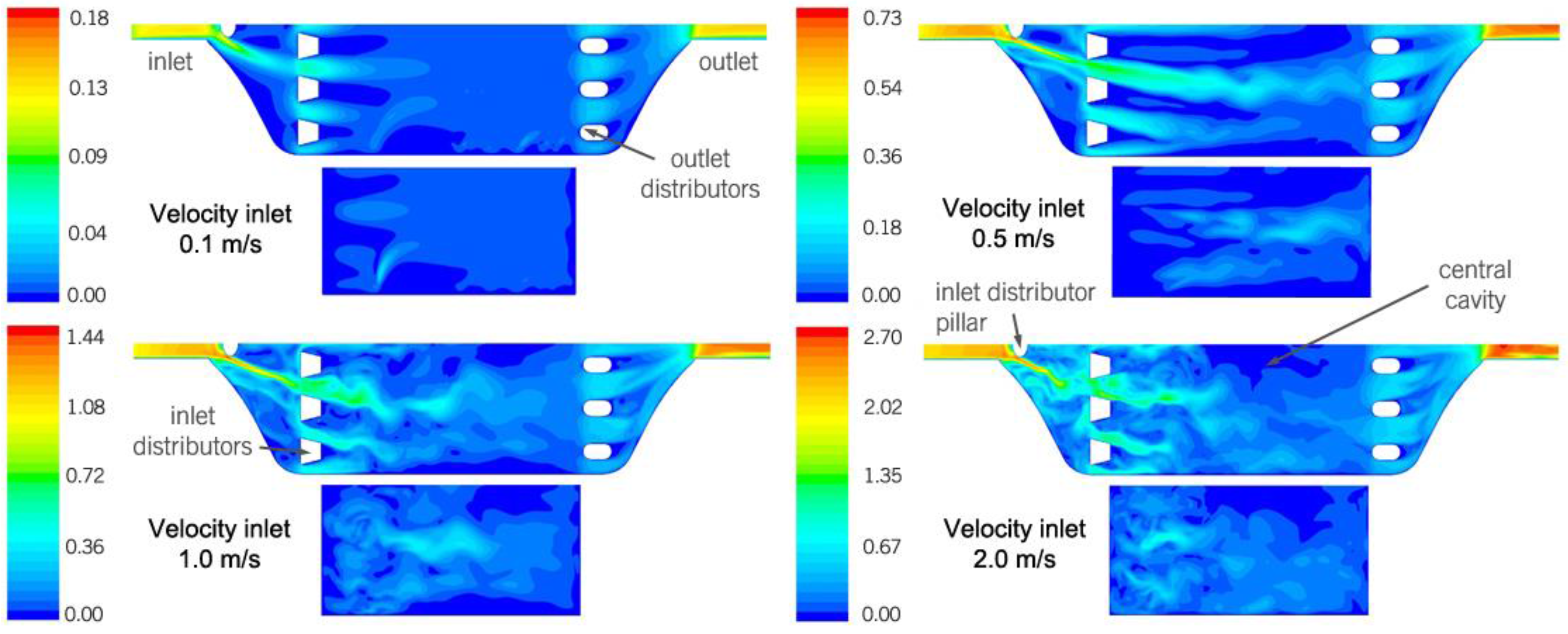
Figure 4 shows the velocity contours for the two planes parallel to the ground: one located at mid-height of the bottom cavity (G0 in Figure 2) and the other at mid-height of the central cavity (G2 in Figure 2).
The central cavity figures show that, in general, the flow inside the central cavity is influenced very little by the distributors at the inlet. This lack of influence can be observed at 0.1 m/s, due to the low velocity: the distributors do not produce significant jets. It can also be observed at 1.0 and 2.0 m/s, due to the high transient nature of the flow, which produces significant velocity magnitudes in all directions, and this in turn reduces the effect of the jets. Only at 0.5 m/s, at which a limited occurrence of the two abovementioned phenomena can be observed, does the influence of the jets produced by the distributors become the most important factor. Clear streamlines, produced by the distributors, can then be observed. The recorded videos confirm this transient behavior.
According to Figure 4, another characteristic that deserves mentioning is the influence of the rounded pillar in front of the inlet designed to distribute the flow. It produces a preferential flow path that goes directly toward the inlet of a certain microchannel. The magnitude of the preferential path depends on the velocity, but only at 0.5 m/s, is the influence clear.
The bottom cavity figures show that there is only a slight influence of the flow along the module in that part. The only effect that influences the flow is the transient behavior, which is significant for all of the studied inlet velocities, except at 0.1 m/s. There is in fact a clear tendency of a stagnant flow near the bottom of the cavity.
Table 3 shows the numerical mean results for the I and G planes, as well as for the entire volume (the mean velocity of all the PEC cell elements of the geometry).
In general, the ratio between the inlet velocity and the mean volume velocity is about 7. Standard deviations are included to show how uniform the velocities are in each plane.
A clear difference can be observed between the 0.1 m/s case and the others for the I planes (parallel to the inlet plane). In the first case, the velocity magnitudes in the three planes are almost the same, but important differences can be observed for the other cases. Plane I1 always shows a greater velocity magnitude than I2 and I3. Moreover, it has the largest standard deviation, because of the remarkable influence of the initial distributors and the rounded pillar. It should be noted that the mean velocities at these planes are not the same, because the magnitude considers all the velocity components.
As far as the G planes are concerned (parallel to the ground plane), plane G2 shows the largest velocity in all cases, because of the direct influence of the inlet. No large differences can be observed between the velocity magnitudes of the G1, G2 and G3 planes. However, a significant velocity divergence can be observed when the velocity magnitude of these planes is compared with the velocity of G0. In all the cases, the velocity magnitude in G0 is much lower, thus indicating that a clear stagnant region exists in the bottom cavity. This hypothesis is also supported by the fact that the standard deviations of the G0 planes are much lower than the others.
The results pertaining to the stagnant zones show that the cases with lower inlet velocities exhibit larger areas, with velocities below 10% of the mean, that is, near the lateral walls and behind the distributors. The case of the inlet velocity of 0.5 m/s is in particular different, due to the influence of the preferential jet caused by the rounded pillar in front of the inlet. Overall, stagnation is never more important in the cases with larger inlet velocities. A final consideration that affects all the analysis pertains to the transient nature of the flow, which produces variations of the flow over time.
Influence of the Geometry
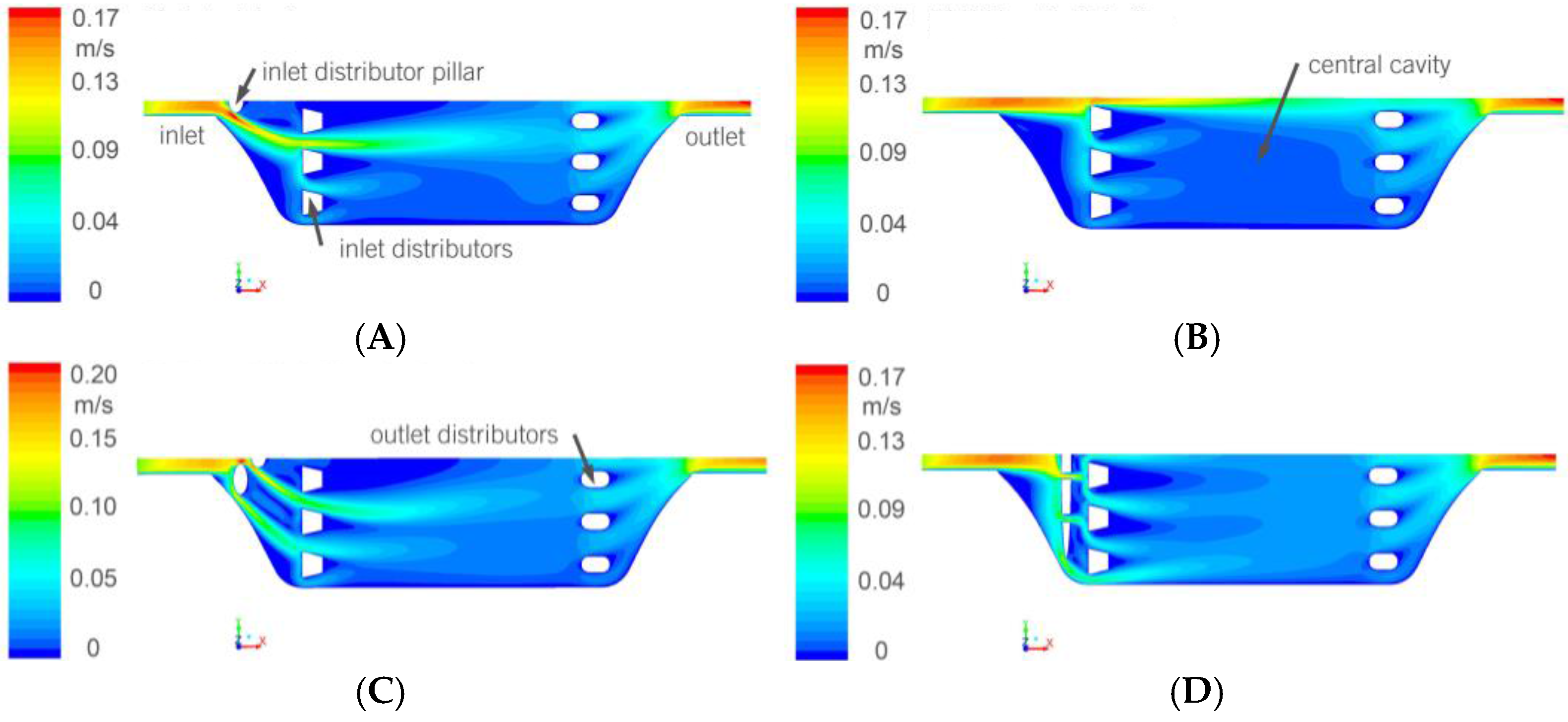
Simulations were performed to establish the influence of the geometry of the PEC cell, as indicated in Figure 1. Different heights inside the cell were considered in order to simulate possible changes on the dimension of the cell that could be necessary due to fabrication issues or to guarantee a good robustness of the device (i.e., to avoid the bending of the cell caused by its heating with the sunlight). The differences in height led to changes in the total cell volumes. The volume of the original model was 984 mm3. Volumes of 1351, 2060, 2736 and 2990 mm3 were adopted for A1, A2, A3 and A4, respectively. In order to analyze the results, the planes and edges shown in Figure 2 were considered.
In all the cases, the inlet velocity was 0.1 m/s. On the basis of the conclusions on the influence of the velocity (previous section), this was considered to be an optimum velocity.
The results show that there are no clear differences in the flow distribution along the direction of the fluid flow. The preferential path created by the rounder pillar is slightly more stressed. Moreover, the magnitude of the vectors decrease as the volume of the PEC cell becomes larger, although their direction does not vary significantly.
Relevant differences can instead be observed in the perpendicular direction (along the planes parallel to the inlet plane). There are very few differences between the original model A and the A1 geometry, where only the central cavity height was increased. However, when the height of the bottom cavity is increased (A2 and A3), significant differences in the velocity magnitude can be observed, although there is still a similarity between the original cases, A1 and A2, as far as the boundary layers at the top and bottom walls are concerned. On the other hand, the situation changes significantly in A3, where a significant layer of stagnant fluid can be observed over the bottom surface.
The A4 flow characteristics are different, and show similarities with and differences from the other cases. The velocity magnitude range is much lower than in the other cases. In the other cases, there are zones of up to approx. 1.8 × 10⁻² m/s, but the maximum velocity in A4 is around 1 × 10⁻² m/s. This lower velocity makes the flow more stagnant, and leads to fewer differences in the magnitude and in the decrease of the stagnant layer over the bottom surface (which is naturally also due to the difference in geometry).
In order to further check the abovementioned differences, Figure 5 shows the velocity profiles along the vertical direction for the 4 alternatives and in four different lines, as indicated in Figure 2. It can clearly be observed that the lowest velocity magnitudes are in the alternative 4 (A4). In addition, the parabolic shapes in A1 are lost in the other cases, as the total height increases.
Figure 6 shows the pathlines of several configurations in order to assess the importance of the stagnation in the alternative geometries.
In general, it can be observed that there is almost no stagnation in the original geometry or in A1. The first indications that stagnation occurs can be observed in A2, but it is particularly evident in A3, where more stagnation occurs. The change in geometry in A4 makes this phenomenon decrease.
Table 4 shows the mean velocities and standard deviations for each plane for the different cases and for the entire volume (the mean velocity of all the PEC cell elements of the geometry A indicated in Figure 2).
The mean volume velocity results decrease as the PEC cell model becomes larger; A4 in fact shows the lowest values. The mean velocity of A1 is 70% of the original case, and is 47%, 38% and 33% for A2, A3 and A4, respectively. The standard deviations show how different the velocities in the plane are (calculated from the velocities at each plane cell). Figure 7 shows that a power regression is the best function that correlates the mean velocity inside the module and its volume.
The results regarding the I planes are proportional to the original case, but also show the abovementioned overall velocity reduction as the PEC cell cavity becomes larger. In all the cases, the I1 plane has the largest velocity magnitudes and standard deviations, due to the inlet effect.
The results pertaining to the G planes clearly show that the planes located at the height closest to the inlet one have the largest velocities. The velocity differences among the G planes are also clear. For example, the ratios between G2 and G00 range from 5.8 to 8.5. It is also interesting to note that, while the maximum velocity is located at G3 for the A1, A2 and A4 cases, it is located at G1 for A3.
Influence of the Initial Distributors
The previous results pointed out the critical effects that the initial flow distributors introduce. These distributors are needed to avoid direct streamlines from the inlet to the outlet, and to avoid stagnation inside the cell. Several geometries were considered and simulated to check their impact on flow spreading inside the cell. Figure 8 shows the different velocity contours for the different designs. The results show that a good design can be obtained by combining two rows of distributors aligned according to Figure 7D. This would facilitate flow homogenization, although a slight increment of the pressure drop would also be produced.
3.1.2. Geometry B (Geometry with Channels)
The only variable that was studied in this model of PEC cell was velocity. The considered velocities were 0.1, 0.5, 1 and 2 m/s, as in geometry A.
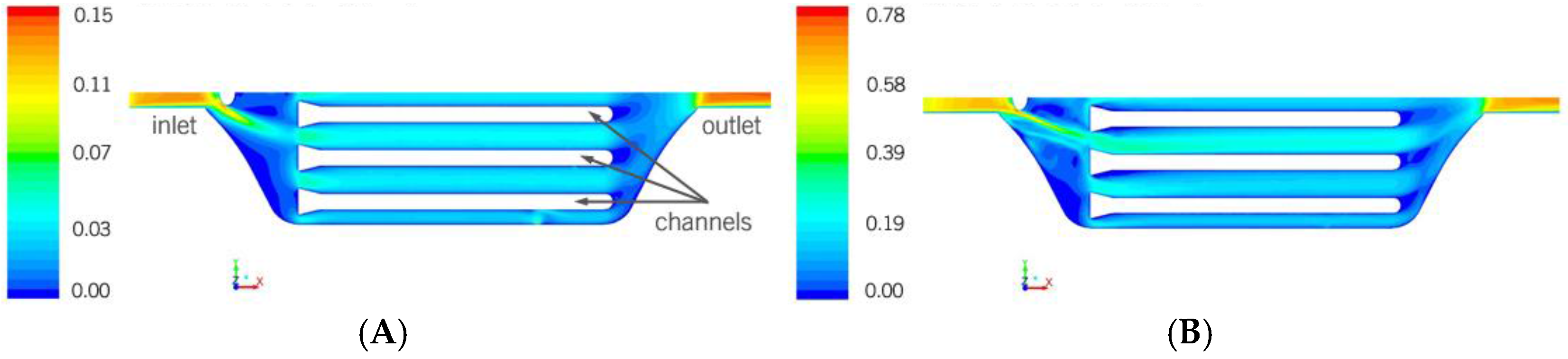
In this case, and unlike geometry A, the flow is much more constrained because of the presence of the microchannels. There is less difference in velocity inside the module, and the flow continues to develop along the microchannels until the inlet velocity exceeds 1 m/s. Thus, an advantage of this PEC cell model is that the stagnant zones are minimized, although the contact surface area of the module could also be lower, because the channel wall width can cover a part of the catalyst surface area limiting the water oxidation reaction on such area.
The results pertaining to the transient behavior of the fluid show that the flow is still stationary in all the module parts for 0.5 m/s. A clear transient zone can be observed at the inlet cavity for 1 m/s, but the flow remains stationary inside the microchannels. The flow is significantly transient for 2 m/s, and has not developed in any of the microreactor zones, including the microchannels (although the magnitude differs because of the microchannels).
A common characteristic of all the cases is the preferential fluid path (Figure 9). The rounded pillar in front of the inlet creates a jet that goes directly toward the inlet of a microchannel. The magnitude of the preferential path depends on the velocity. The faster the fluid is injected, the greater the difference between the channel flow distributions. The effect is not so obvious for 0.1 m/s, but it starts to be significant from 0.5 onwards.
The results concerning the direction perpendicular to the fluid flow show that the fluid is developed for 0.1 m/s in all the microchannels, and the velocities are similar. Significant differences start to occur between the different microchannels for 0.5 m/s. Non-developed fluid flow symptoms also arise as non-symmetric shapes appear in the velocity magnitude contours. The abovementioned situation can clearly be observed for 1 m/s, and it increases even more for 2 m/s. An important change occurs between 0.5 and 1 m/s.
Some numerical data were extracted from the simulation at the different representative control planes defined in Figure 2B.
Table 5 shows the mean velocities and standard deviations of each plane, for the different studied inlet velocities, and for the entire volume (i.e., the mean velocity of all the cell elements of the geometry).
The ratio between the inlet velocity and the mean volume velocity is about 4 (almost the half of the values observed for the geometry A), with a decreasing tendency as the inlet velocity increases. This tendency is similar to the behavior that was observed for geometry A, but the mean velocity values for model A are almost one order of magnitude lower than those for geometry B. This indicates that model A shows a more stagnant tendency because of the bottom cavity. Thus, as far as this feature is concerned, model B is better.
It can be noted, for the I planes (parallel to the inlet plane), that although I2 and I3 always show the same velocity, I1 is large for all the cases, except for the one related to 0.1 m/s. This confirms the change in the fluid behavior between 0.1 and 0.5 m/s. It should be noted that the mean velocities at these planes are not the same, because the magnitude considers all the velocity components.
As far as the G planes are concerned (parallel to the ground plane), the G2 plane shows the greatest velocity in all the cases, as it corresponds to the central one inside the microchannels. A difference can also be observed between 0.1 m/s and the others: although the other velocities at G1 and G3 are similar and lower than G2, G3 is closer to G2 than to G1 for 0.1 m/s. It should be pointed out that, in all the cases, G1 (the plane closest to the bottom surface) does not have a significantly low velocity, compared with the mean velocity. Proportional values of the standard deviation were obtained for all the cases.
The results regarding the stagnant zones show that, as the inlet velocity decreases, more of the flow area is under a lower velocity magnitude than 10% of the mean. However, almost all the sectors where there are stagnant zones are at a certain distance from the microchannels where the reaction occurs. In other words, there are almost no stagnant zones in the region of interest. Fluid that is more stagnant can be observed in the microchannel zones for high velocities. Therefore, it is only in the case of 0.5 m/s, which no fluid is found under a 10% of the mean volume velocity in the zone. Nevertheless, it should be noted that, in absolute terms, stagnation is never important in the cases with higher inlet velocities. In all the studied cases pertaining to the microchannel zones there are no elements with a velocity magnitude below 0.005 m/s, although stagnant zones are observed in the region of the PEC cell where the channels are not present.
3.1.3. Summary of the Hydrodynamic Results
As far as geometry A is concerned, an inlet velocity of 0.5 m/s (6.4 L/h) should be avoided, because of the presence of a preferential jet in front of the inlet, produced by the round pillar. That behavior has consequences on all the module zones, including the bottom cavity, because more differences in the vortices and in the magnitude of the velocity are observed. An alternative solution could be to make some changes to the design of the rounded pillar. The case with the lowest inlet velocity (0.1 m/s) clearly offers more velocity homogeneity, in terms of magnitude and direction. This is the only studied situation in which this effect has emerged. However, this case can also suffer from a drawback: a very low fluid velocity magnitude (0.7 × 10⁻² m/s in plane G0). The importance of this low magnitude should be evaluated, but its effect may not be so important. A low velocity may enhance the reaction rate, if the catalytic surface is not covered with the produced bubbles, which can limit the catalytic activity. In this case, an inlet velocity of 0.1 m/s (1.3 L/h) would be the optimum one. In the contrary case, an inlet velocity higher than 0.5 m/s should be selected (with the present pillar design).
There are no relevant differences in the hydrodynamic behavior of the flow inside the module between 1 and 2 m/s. However, the velocity magnitude obviously changes overall as the inlet velocity changes. Thus, a suitable velocity would be the one achieved after the inlet velocity is increased from 0.5 m/s to the value at which the rounded initial pillar effect diminishes (between 0.5 and 1 m/s).
As the volume of the module increases (geometry A and its alternatives A1 to A4), the overall mean velocity inside decreases (therefore the lowest decrement occurs for A1, see Section 3.1.1 (Influence of the Geometry)). As far as the flow distribution is concerned, A1 does not show any significant differences in hydrodynamics compared to the original case. Variances start to be noted for A2, and are observed in the vertical velocity profile as well as some stagnant zones in the corner parts of the bottom cavity of the module. This is the case of A3, where major differences are encountered, especially in the presence of stagnant fluid over the bottom wall of the module. A4, which has the same height as A3, but a different cavity distribution, mitigates the stagnation issue of A3, but reduces the mean velocity inside the geometry even more.
The results obtained for geometry B, considering the studied parameters, make it possible to state that a change in behavior can be observed between 0.5 and 1 m/s. Fluid uniformity is lost inside the microchannels at high velocities: different fluid distributions in the channels, a transient flow, a more undeveloped flux or a turbulence increment can be observed. For these reasons, working at velocities lower than 0.5 m/s (6.4 L/h) may be adequate, if the coverage of the catalytic surface with the formed bubbles is low. Another reason for recommending working below 0.5 m/s is connected to avoiding the effect of the initial distributor located just after the inlet, which causes a jet to form. At high velocities, the jet continues to develop toward the entrance of a particular channel, and thus generates a preferential path. It produces a significant non-uniform flow distribution along all the microchannels. There are almost no stagnant zones and the effect of velocity is low.
3.2. Bubble Formation and Removal
Oxygen and protons are produced during the water splitting reaction. Oxygen forms as bubbles that quickly coalesce from the pores of the catalyst to the bulk solution (water) inside the cell. Because of the surface tension and wall adhesion forces, the oxygen bubbles have the tendency to remain attached to the catalyst wall [22]. This makes the catalyst lose contact with the water. The consequence is that the water splitting reaction stops. In order to improve catalyst efficiency, it is necessary to remove the oxygen bubbles from the cell. Some ways of sweeping the bubbles out from the cell are: controlling the speed of the liquid and orienting the cell according to gravity.
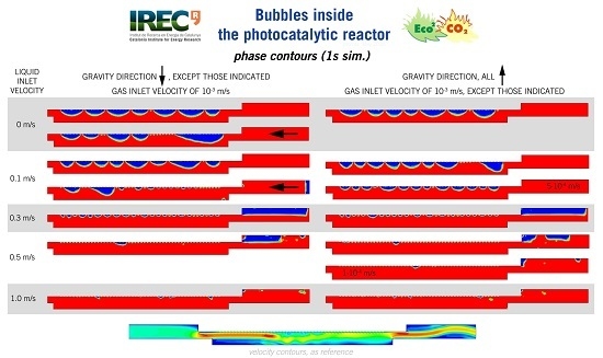
Several simulations were performed to assess the bubble removal process considering the aforementioned factors, and the influence of the liquid velocity inside the cell and the gravity direction were studied. The influence of the oxygen production rate was also studied. Figure 10 summarizes the obtained results. The results are expressed in terms of liquid and gas fraction related to the entire volume.
The results show three types of behavior that depend on the liquid inlet velocity. When the liquid is stagnant, all the oxygen remains in the cell after 1 s. Buoyancy on its own is not enough to detach the bubbles from the catalytic surface. Nevertheless, the results show that gravity could play an important role in facilitating bubble removal if used in the correct direction relative to the outlet. The accumulation of oxygen inside the cell, after 1 s, is still remarkable for a low liquid inlet velocity, except for the case where the gravity direction is more favorable (against the outlet). In this case, bubbles are removed. The bubbles are removed quickly and independently of the gravity direction for a liquid inlet velocity of 0.3 m/s and higher. The liquid velocity also ensures that the oxygen bubbles are removed just as they enter the cell, and this helps prevent coalescence. Thus, a high liquid velocity not only leads to better bubble removal, but also prevents large bubbles from forming, which instead occurs for a stagnant liquid and for low liquid inlet velocities.
Table 6 shows the mean numerical results of the oxygen fraction and the mean liquid velocities in the simulated surface. The results show that the gas fraction decreases when the velocity inside the cells increases, when gravity is opposite the flow direction and when less oxygen is produced.
3.2.1. Influence of the Liquid Velocity
Five liquid velocity inlets were considered to assess the effects of the liquid velocity on bubbles removal: 0 (stagnant fluid), 0.1, 0.3, 0.5 and 1.0 m/s. The main monitored parameter was the oxygen fraction, and it was monitored in several control lines (as shown in Figure 3). Figure 11A shows this parameter in different control lines as a function of the inlet velocity after one simulated second.
A notable influence of the inlet velocity can be observed for the h4a control line (the nearest to the catalyst surface). First, as the velocity increases, the oxygen fraction decreases in a non-linear manner. No great difference is observed from 0 to 0.1 m/s, while a difference can instead be observed from 0.1 to 0.3 m/s. A great difference can also be noted from 0.3 to 0.5 m/s, but not from 0.5 to 1.0 m/s. Thus, the 0.1 to 0.5 m/s range is the one that causes significant changes in the oxygen fraction and consequently in the growing of bubbles after their formation: almost no bubbles are removed below 0.1 m/s, while most of the bubbles are expulsed from 0.5 m/s onwards.
It can be observed that the oxygen fraction, in the h3a control line, drops to half when the liquid inlet velocity changes from 0 (a stagnant fluid) to 0.1 m/s. At 0.3 m/s, the oxygen fraction is almost 0, which means that no oxygen bubbles are in that zone. Therefore, there is no need to increase the velocity after 0.3 m/s is reached. Other control lines, such as h4b and v3, confirm this result. The oxygen fraction at 0.3 m/s is still high in the v5 and h5 control lines, but this is due to some stagnant oxygen remaining in the outlet part of the reactor (see h5) that is located outside the reactive zone.
Finally, it should be pointed out that the oxygen fraction in v5, h5 and h4b is zero for the stagnant fluid, because all the formed oxygen remains attached to the catalytic surface.
3.2.2. Influence of the Gravity Direction
Three gravity directions were considered to assess the effects of gravity on the removal of bubbles (GC, GF and GM, as previously described in Section 2.1.2). GC (gravity with same direction as the gas inlet) was found to be the most unfavorable direction, as it facilitates the attachment of gas bubbles to the catalytic wall. The main monitored parameter once again was the oxygen fraction, which was analyzed in several control lines. Figure 11B shows this parameter in different control lines as a function of the gravity direction, and for two different inlet liquid velocities: 0 (stagnant fluid) and 0.1 m/s. The obtained results show that gravity has almost no influence at higher velocities (the liquid velocity is the dominant variable).
In general, the differences pertaining to the gravity direction are not so large. The largest differences were found for the stagnant liquid fluid and the GM case. That gravity direction (i.e., contrary to the liquid inlet direction) is the one that clearly helped the bubbles exit the cell. This result was observed in the v1, v2, v3 and v4 control lines. The oxygen fraction in v1 and v2 was much lower for GM than for GC and GF (gravity with opposite direction as the gas inlet), while it was much higher in v3. This is because the bubbles in the GM case can be removed, but they did not do so in the GC and GF cases. In the GM case, not only did more bubbles reach v3 but they also reached v4, where the presence of oxygen was not detected for the GC and GF cases.
The liquid velocity inside the cell and gravity are the two main variables that can be set to affect the removal of bubbles. Curve fittings were made from the obtained results in order to check whether there was any kind of correlation between those parameters and the oxygen fraction in any of the key control lines. A factor obtained by multiplying the liquid inlet velocity by the gravity (set to 1 for the GC cases and 1.1 for the GF ones) was plotted against the oxygen fraction for the h3a and h4a control lines. The best correlation was obtained through the fitting with a power function, for which a R2 higher than 0.94 was obtained, as Figure 12 shows. This result confirmed the predominant effect of the liquid velocity.
3.2.3. Oxygen Production Rate
The oxygen production rate also influences the amount of oxygen remaining in the cell. This rate does not correspond to a process variable but to a process yield and, obviously, depends on the catalyst material. In order to consider different possible yields, five different gas inlet velocities were analyzed (1 × 10⁻¹, 1 × 10⁻², 1 × 10⁻³, 5 × 10⁻⁴, 1 × 10⁻⁴ and 1 × 10⁻⁵ m/s). The liquid inlet velocity and gravity direction were fixed at 0.5 m/s and GF, respectively. Figure 11C shows the oxygen fractions for several control lines.
In general, the results show that no oxygen is produced at the lowest velocity (10−5 m/s) or within the simulated frame time. Relative differences were observed for the other cases, although they were not reflected in absolute values.
The h4a results (that is, for the control line nearest to the catalytic surface) show the influence of this variable and its non-linear behavior: there is a larger difference between 1 × 10⁻³ and 5 × 10⁻⁴ m/s (half velocity) than between 5 × 10⁻⁴ m/s and 1 × 10⁻⁴ m/s (five times lower). The results for the other control lines are similar, except for h5. This control line is located outside the reactive part, where the oxygen accumulates, as already mentioned above. The oxygen fraction has the largest values in the accumulation area, and they are very similar for the 1 × 10⁻³ and 5 × 10⁻⁴ m/s cases. There is almost no oxygen for the other situations or in this control line, because of the low oxygen production rate.
The high oxygen inlet velocity (1 × 10⁻¹ and 1 × 10⁻² m/s) as well as the conditions of a stagnant liquid accelerate the gas bubbles coalescence and cause the formation of large bubbles inside the cell. Oxygen leaves the cell at a steady state, but a large concentration (large bubbles) of oxygen remains inside the cell (at 0.52 s, the mean oxygen concentration on the 2D face is 0.70). In these conditions, the hypothesis of a constant oxygen inlet velocity cannot be considered reliable because once the catalytic surface is completely covered, no more oxygen will be produced. Nevertheless, the results are useful, because they indicate that although a large bubble could not increase inside the cell, it would remain attached to the catalytic surface without leaving the cell, despite the influence of gravity.
3.2.4. Comparison of the 2D and 3D Simulation Results
One 3D simulation was performed to check the 2D results when a relevant third dimension size, in agreement with the bubble size, was considered. Table 7 shows some comparative results and Figure 13 shows contour diagrams regarding the static pressure, velocity magnitude and oxygen fraction for both cases.
If the contour diagrams are examined, it can be seen that very similar profiles are obtained for the velocity and pressure. Differences regarding the position of the bubbles on the fraction contours emerge, but they are mainly due to the unsteady behavior of the flow. Nevertheless, the size of the bubbles and the coalescence level are very similar. This correspondence is also obtained for the numerical values. Because of the limited thickness of the 3D volume, the mean results pertaining to the catalytic surface are very close to the mean results pertaining to the whole volume.
3.2.5. Experimental Validation of the Simulation Results
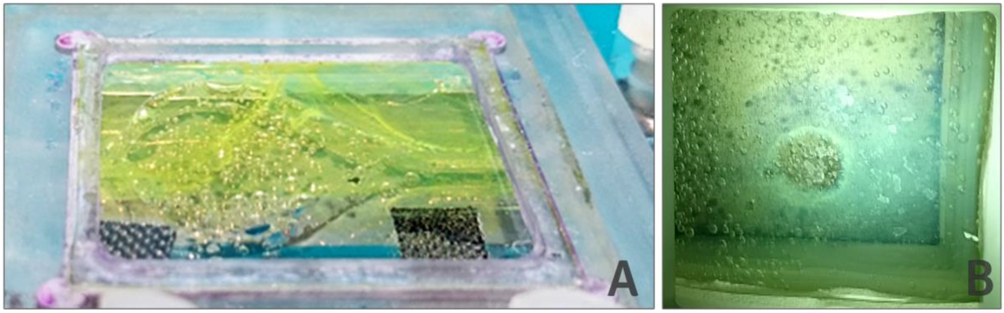
The results obtained in these simulations were compared with observations from several experiments. Videos were made in which bubbles and their movement inside the cell were recorded. Figure 14 shows the obtained images for different liquid velocities, where different bubble sizes can be observed. Large bubbles were obtained for the stagnant liquid case. Two types of bubbles can be observed for the circulating liquid case (1 m/s): medium-sized bubbles attached to the surface (mean size of 0.57 mm and standard deviation of 0.14 mm) and small bubbles circulating in the bulk solution and moving toward the outlet (mean size of 0.21 mm and standard deviation of 0.01 mm). These results are in agreement with those obtained in the simulations. The results shown in Figure 11B could fit better with simulations performed at a higher inlet liquid velocity than 2 m/s. However, these discrepancies were to be expected, considering the several limitations and hypothesis considered, such as the model used in the simulations (bubble generator), the difficulty of correctly assessing the exact gas inlet velocity in the experiments, the changes in the reaction yield due to surface coverage and the possible thermal effects due to light irradiance.
4. Conclusions
CFD simulations have been used to assess the process design and cell configuration of a photo-electrochemical (PEC) cell in which water is split into protons and oxygen on a catalytic surface.
From the hydrodynamic point of view, the purpose of a PEC cell is not to mix components but to facilitate the reaction on the catalyst surface. A regular distribution of the liquid phase over the catalyst surface is necessary, and stagnant zones should be avoided. Turbulence may also be a drawback, as it may lead to a non-regular fluid distribution. The shear stress caused by the motion of a liquid should allow oxygen bubbles to be dragged out of the cell. If the bubbles are not removed from the cell, they remain attached to the catalytic surface, thus preventing the reaction from occurring because the water is not able to wet the catalyst.
Channeled cells boost flow uniformity inside a cell, but the presence of channels can lead to a reduction in the active catalytic surface and can diminish the yield. Suitable initial distributors (i.e., two layered A/B geometry as previously explained) may be used to overcome these issues. Incrementing the thickness of the cell does not improve the hydrodynamics or the reaction yield, and the cell wall should be kept as thin as possible (no thicker than 3 mm) to avoid stagnant zones.
An inlet liquid velocity equal to or higher than 1.5 m/s may be used to avoid the coalescence of oxygen bubbles, and to drag them to the cell outlet. Gravity does not play a significant role at these velocities, and the orientation of the cell is not relevant. The magnitude of these velocities minimizes the effects of the preferred paths created by the initial distributors. Although the flow begins to show turbulent behavior, a reasonably regular liquid distribution inside the cell is maintained. In this way, the negative issues encountered in the hydrodynamic study can be avoided for the inlet liquid velocity. The here presented results can be used as guidelines for the optimum design of photocatalytic cells for the water splitting reaction for the production of solar fuels, such as H2 or other CO2 reduction products (i.e., CO, CH4, among others).
Supplementary Materials
Supplementary File 1Acknowledgments
The authors would like to thank the European Commission, 7th Framework Program (NMP-2012 Project ECO2CO2 No. 309701), for the financial support. The authors would also like to acknowledge the Spanish Ministry of Economy and Competitiveness for the financial support through the CTQ2014-56285-R project. The research was also supported by European Regional Development Funds (ERDF, FEDER Programa Competitividad de Catalunya 2007–2013). The authors would like to thank Alessandro Monticelli for his support in defining the cells that were modeled in this work.
Author Contributions
Carles Torras designed and performed the simulations, analyzed the results and wrote the paper. Esther Lorente contributed by analyzing the results and helped to write the paper. Simelys Hernández formulated the problem, performed the experiments and helped to write the paper. Nunzio Russo contributed by formulating the problem, and by discussing and analyzing the results. Joan Salvadó contributed by analyzing the results and helped to write the paper.
Conflicts of Interest
The authors declare no conflict of interest.
References
- Kalyanasundaram, K.; Graetzel, M. Artificial photosynthesis: Biomimetic approaches to solar energy conversion and storage. Curr. Opin. Biotechnol. 2010, 21, 298–310. [Google Scholar] [CrossRef] [PubMed]
- Izumi, Y. Recent advances in the photocatalytic conversion of carbon dioxide to fuels with water and/or hydrogen using solar energy and beyond. Coord. Chem. Rev. 2013, 257, 171–186. [Google Scholar] [CrossRef]
- Xiang, C.; Papadantonakis, K.M.; Lewis, N.S. Principles and implementations of electrolysis systems for water splitting. Mater. Horiz. 2016, 3, 169–173. [Google Scholar] [CrossRef]
- Jhong, H.-R.M.; Ma, S.; Kenis, P.J.A. Electrochemical conversion of CO2 to useful chemicals: Current status, remaining challenges, and future opportunities. Curr. Opin. Chem. Eng. 2013, 2, 191–199. [Google Scholar] [CrossRef]
- Ronge, J.; Bosserez, T.; Martel, D.; Nervi, C.; Boarino, L.; Taulelle, F.; Decher, G.; Bordiga, S.; Martens, J.A. Monolithic cells for solar fuels. Chem. Soc. Rev. 2014, 43, 7963–7981. [Google Scholar] [CrossRef] [PubMed]
- Ager, J.W.; Shaner, M.R.; Walczak, K.A.; Sharp, I.D.; Ardo, S. Experimental demonstrations of spontaneous, solar-driven photoelectrochemical water splitting. Energy Environ. Sci. 2015, 8, 2811–2824. [Google Scholar] [CrossRef]
- Tolod, K.; Hernández, S.; Russo, N. Recent advances in the BiVO4 photocatalyst for sun-driven water oxidation: Top-performing photoanodes and scale-up challenges. Catalysts 2017, 7, 13. [Google Scholar] [CrossRef]
- Park, Y.; McDonald, K.J.; Choi, K.-S. Progress in bismuth vanadate photoanodes for use in solar water oxidation. Chem. Soc. Rev. 2013, 42, 2321–2337. [Google Scholar] [CrossRef] [PubMed]
- Kang, D.; Kim, T.W.; Kubota, S.R.; Cardiel, A.C.; Cha, H.G.; Choi, K.-S. Electrochemical synthesis of photoelectrodes and catalysts for use in solar water splitting. Chem. Rev. 2015, 115, 12839–12887. [Google Scholar] [CrossRef] [PubMed]
- Hernandez, S.; Hidalgo, D.; Sacco, A.; Chiodoni, A.; Lamberti, A.; Cauda, V.; Tresso, E.; Saracco, G. Comparison of photocatalytic and transport properties of TiO2 and zno nanostructures for solar-driven water splitting. Phys. Chem. Chem. Phys. 2015, 17, 7775–7786. [Google Scholar] [CrossRef] [PubMed]
- McCrory, C.C.L.; Jung, S.; Peters, J.C.; Jaramillo, T.F. Benchmarking heterogeneous electrocatalysts for the oxygen evolution reaction. J. Am. Chem. Soc. 2013, 135, 16977–16987. [Google Scholar] [CrossRef] [PubMed]
- Hernández, S.; Tortello, M.; Sacco, A.; Quaglio, M.; Meyer, T.; Bianco, S.; Saracco, G.; Pirri, C.F.; Tresso, E. New transparent laser-drilled fluorine-doped tin oxide covered quartz electrodes for photo-electrochemical water splitting. Electrochim. Acta 2014, 131, 184–194. [Google Scholar] [CrossRef]
- Saracco, G.; Barbero, G.; Hernández, S.; Alexe-Ionescu, A.L. Non-monotonic dependence of the current density on the thickness of the photoactive layer. J. Electroanal. Chem. 2017, 788, 61–65. [Google Scholar] [CrossRef]
- Hara, K.; Sakata, T. Large current density CO2 reduction under high pressure using gas diffusion electrodes. Bull. Chem. Soc. Jpn. 1997, 70, 571–576. [Google Scholar] [CrossRef]
- Kaneco, S.; Iiba, K.; Katsumata, H.; Suzuki, T.; Ohta, K. Electrochemical reduction of high pressure carbon dioxide at a Cu electrode in cold methanol with CsOH supporting salt. Chem. Eng. J. 2007, 128, 47–50. [Google Scholar] [CrossRef]
- Hernandez, S.; Farkhondehfal, M.A.; Sastre, F.; Makkee, M.; Saracco, G.; Russo, N. Syngas production from electrochemical reduction of CO2: Current status and prospective implementation. Green Chem. 2017. [Google Scholar] [CrossRef]
- Choi, P.; Bessarabov, D.G.; Datta, R. A simple model for solid polymer electrolyte (SPE) water electrolysis. Solid State Ion. 2004, 175, 535–539. [Google Scholar] [CrossRef]
- Jeng, K.-T.; Liu, Y.-C.; Leu, Y.-F.; Zeng, Y.-Z.; Chung, J.-C.; Wei, T.-Y. Membrane electrode assembly-based photoelectrochemical cell for hydrogen generation. Int. J. Hydrog. Energy 2010, 35, 10890–10897. [Google Scholar] [CrossRef]
- Reece, S.Y.; Hamel, J.A.; Sung, K.; Jarvi, T.D.; Esswein, A.J.; Pijpers, J.J.H.; Nocera, D.G. Wireless solar water splitting using silicon-based semiconductors and earth-abundant catalysts. Science 2011, 334, 645–648. [Google Scholar] [CrossRef] [PubMed]
- Hernández, S.; Saracco, G.; Alexe-Ionescu, A.L.; Barbero, G. Electric investigation of a photo-electrochemical water splitting device based on a proton exchange membrane within drilled FTO-covered quartz electrodes: Under dark and light conditions. Electrochim. Acta 2014, 144, 352–360. [Google Scholar] [CrossRef]
- Wu, K.; Birgersson, E.; Kim, B.; Kenis, P.J.A.; Karimi, I.A. Modeling and experimental validation of electrochemical reduction of CO2 to co in a microfluidic cell. J. Electrochem. Soc. 2015, 162, F23–F32. [Google Scholar] [CrossRef]
- Hernández, S.; Barbero, G.; Saracco, G.; Alexe-Ionescu, A.L. Considerations on oxygen bubble formation and evolution on bivo4 porous anodes used in water splitting photoelectrochemical cells. J. Phys. Chem. C 2015, 119, 9916–9925. [Google Scholar] [CrossRef]
- Gliozzi, A.S.; Hernández, S.; Alexe-Ionescu, A.L.; Saracco, G.; Barbero, G. A model for electrode effects based on adsorption theory. Electrochim. Acta 2015, 178, 280–286. [Google Scholar] [CrossRef]
- Li, Y.L.; Lin, P.J.; Tung, K.L. Cfd analysis of fluid flow through a spacer-filled disk-type membrane module. Desalination 2011, 283, 140–147. [Google Scholar] [CrossRef]
- Ratkovich, N.; Chan, C.C.V.; Bentzen, T.R.; Rasmussen, M.R. Experimental and CFD simulation studies of wall shear stress for different impeller configurations and MBR activated sludge. Water Sci. Technol. 2012, 65, 2061–2070. [Google Scholar] [CrossRef] [PubMed]
- Della Torre, A.; Lucci, F.; Montenegro, G.; Onorati, A.; Dimopoulos Eggenschwiler, P.; Tronconi, E.; Groppi, G. CFD modeling of catalytic reactions in open-cell foam substrates. Comput. Chem. Eng. 2016, 92, 55–63. [Google Scholar] [CrossRef]
- Khodaparast, S.; Magnini, M.; Borhani, N.; Thome, J.R. Dynamics of isolated confined air bubbles in liquid flows through circular microchannels: An experimental and numerical study. Microfluid. Nanofluid. 2015, 19, 209–234. [Google Scholar] [CrossRef]
- Farivar, F. CFD simulation and development of an improved photoelectrochemical reactor for H2 production. Int. J. Hydrog. Energy 2016, 41, 882–888. [Google Scholar] [CrossRef]
- Schluckner, C.; Subotić, V.; Lawlor, V.; Hochenauer, C. Three-dimensional numerical and experimental investigation of an industrial-sized SOFC fueled by diesel reformat—Part II: Detailed reforming chemistry and carbon deposition analysis. Int. J. Hydrog. Energy 2015, 40, 10943–10959. [Google Scholar] [CrossRef]
- Escudero González, J.; Alberola, A.; Amparo López Jiménez, P. Redox cell hydrodynamics modelling—Simulation and experimental validation. Eng. Appl. Comput. Fluid Mech. 2013, 7, 168–181. [Google Scholar] [CrossRef]
- Zhang, K.; Feng, Y.; Schwarz, P.; Wang, Z.; Cooksey, M. Computational fluid dynamics (CFD) modeling of bubble dynamics in the aluminum smelting process. Ind. Eng. Chem. Res. 2013, 52, 11378–11390. [Google Scholar] [CrossRef]
- Brackbill, J.U.; Kothe, D.B.; Zemach, C. A continuum method for modeling surface tension. J. Comput. Phys. 1992, 100, 335–354. [Google Scholar] [CrossRef]
- Pallas, N.R.; Harrison, Y. Selected papers from a symposium on recent progress in interfacial tensiometry, held at the third chemical congress of north americaan automated drop shape apparatus and the surface tension of pure water. Colloids Surf. 1990, 43, 169–194. [Google Scholar] [CrossRef]
- Thapper, A.; Styring, S.; Saracco, G.; Rutherford, A.W.; Robert, B.; Magnuson, A.; Lubitz, W.; Llobet, A.; Kurz, P.; Holzwarth, A.; et al. Artificial photosynthesis for solar fuels—An evolving research field within ampea, a joint programme of the european energy research alliance. Green 2013, 3, 43–57. [Google Scholar] [CrossRef]
- Schneider, C.A.; Rasband, W.S.; Eliceiri, K.W. Nih image to imagej: 25 years of image analysis. Nat. Methods 2012, 9, 671–675. [Google Scholar] [CrossRef] [PubMed]
Figure 1.
Geometries of PEC cell simulated in the hydrodynamic study.
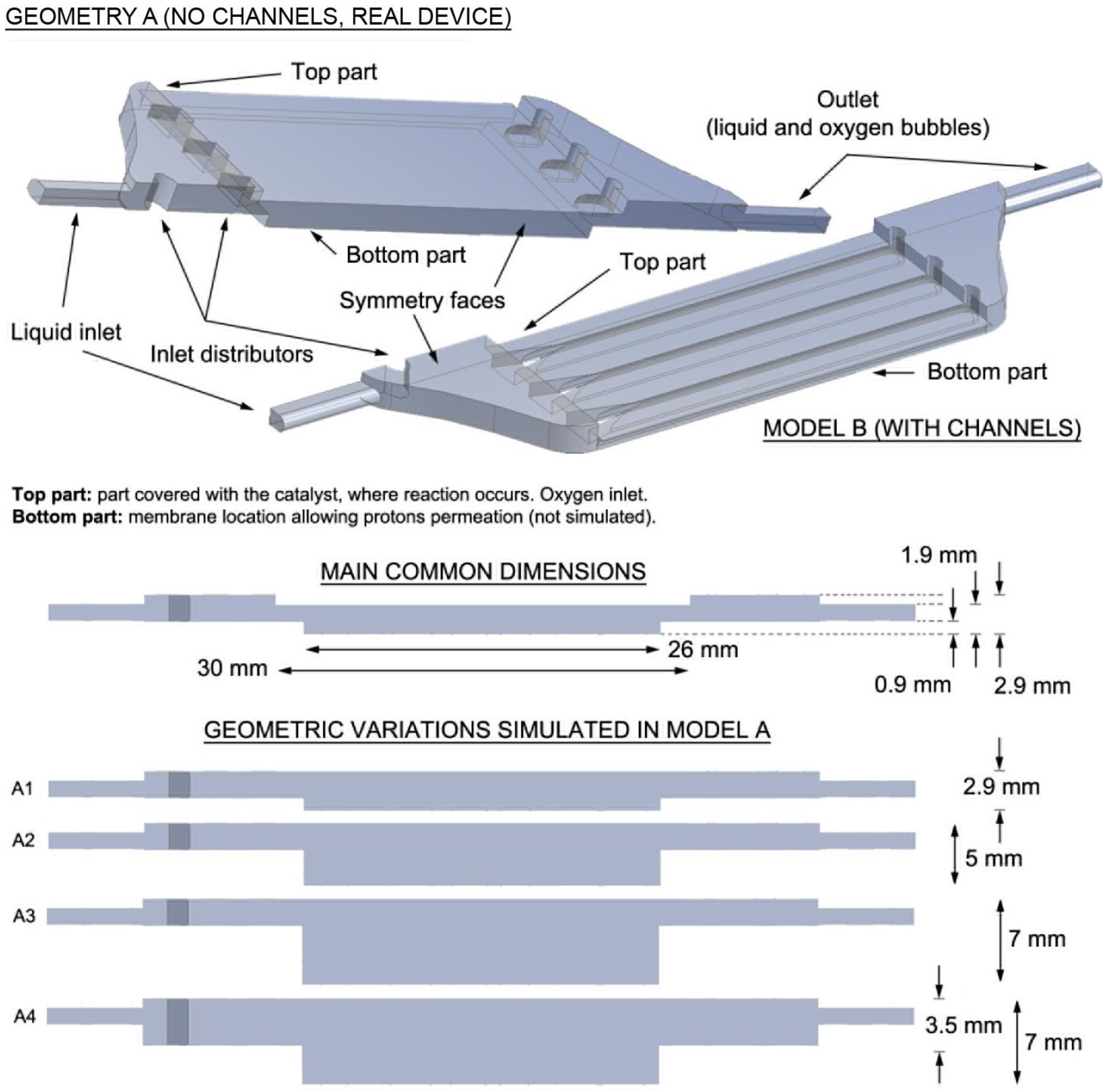
Figure 2.
(A) Control plane locations for geometry A (No channels, real device). I1, I2 & I3: planes parallel to the inlet plane, at x = 4, 15 & 26 mm. G0, G1, G2, G3: planes parallel to the microchannel ground plane, at z = −0.45, 0.25, 0.5 & 0.75 mm. G00 and G4 only included for alternative models (A1 to A4 in Figure 1); (B) Control plane locations for geometry B (With channels). I1, I2 & I3: planes parallel to the inlet plane, at x = 4, 15 & 26 mm. G1, G2, G3: planes parallel to the microchannel ground plane, at z = 0.25, 0.5 & 0.75 mm.

Figure 3.
2D geometry with control lines used to perform the bubbles characterization simulations.

Figure 4.
Velocity contours at two planes parallel to the ground (z = 0.5 mm and z = −0.45 mm) for geometry A for different inlet velocities (0.1, 0.5, 1.0 and 2.0 m/s).
Figure 4.
Velocity contours at two planes parallel to the ground (z = 0.5 mm and z = −0.45 mm) for geometry A for different inlet velocities (0.1, 0.5, 1.0 and 2.0 m/s).

Figure 5.
Scatter plots with the velocity magnitude as a function of the vertical position for the four geometry A alternatives: A1, A2, A3 and A4. Reduction in the mean module velocity as a function of the module volume for an inlet velocity of 0.1 m/s.
Figure 5.
Scatter plots with the velocity magnitude as a function of the vertical position for the four geometry A alternatives: A1, A2, A3 and A4. Reduction in the mean module velocity as a function of the module volume for an inlet velocity of 0.1 m/s.
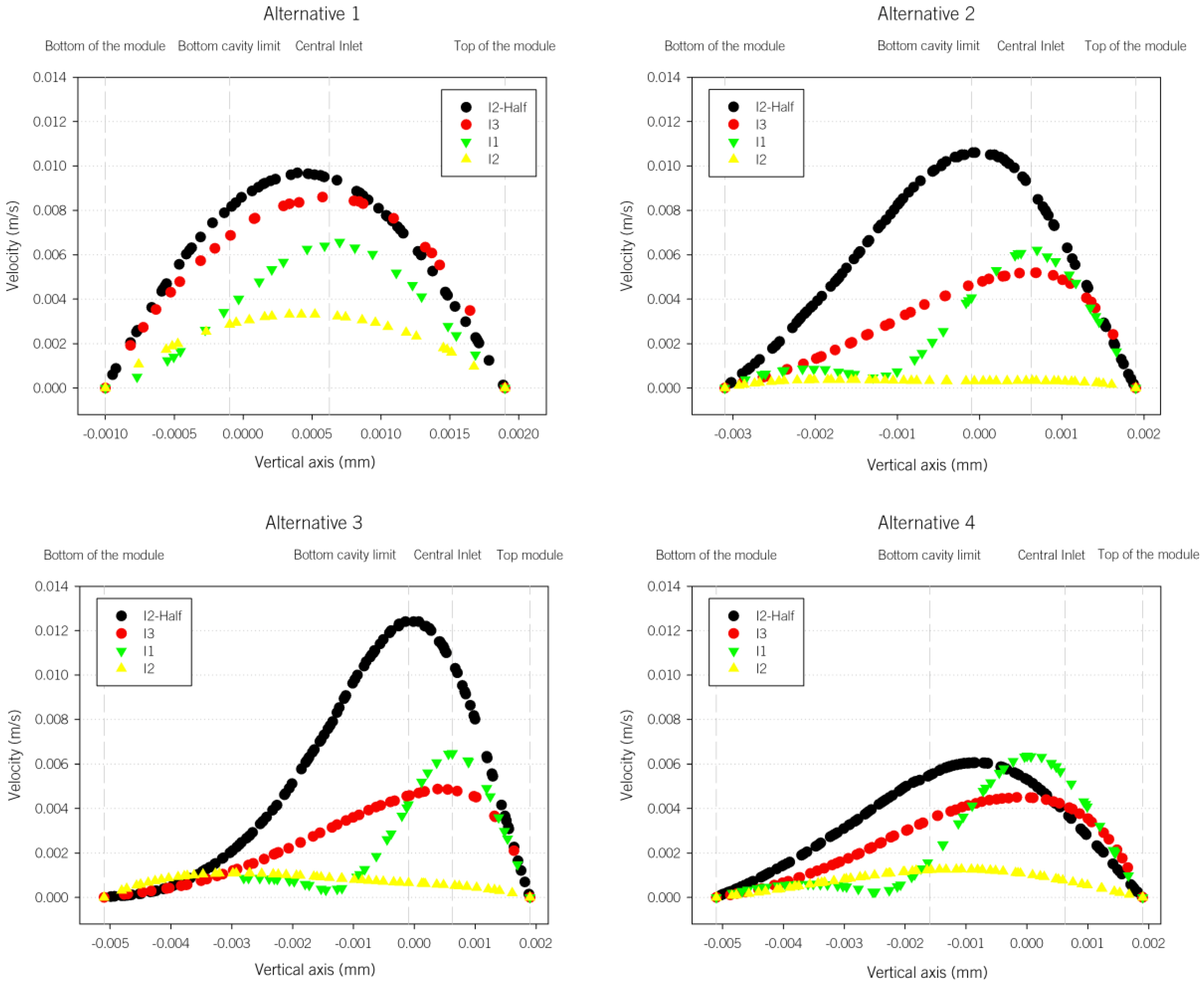
Figure 6.
Pathlines of the alternative geometries for the height study in model A (the different colors represent different paths).
Figure 6.
Pathlines of the alternative geometries for the height study in model A (the different colors represent different paths).
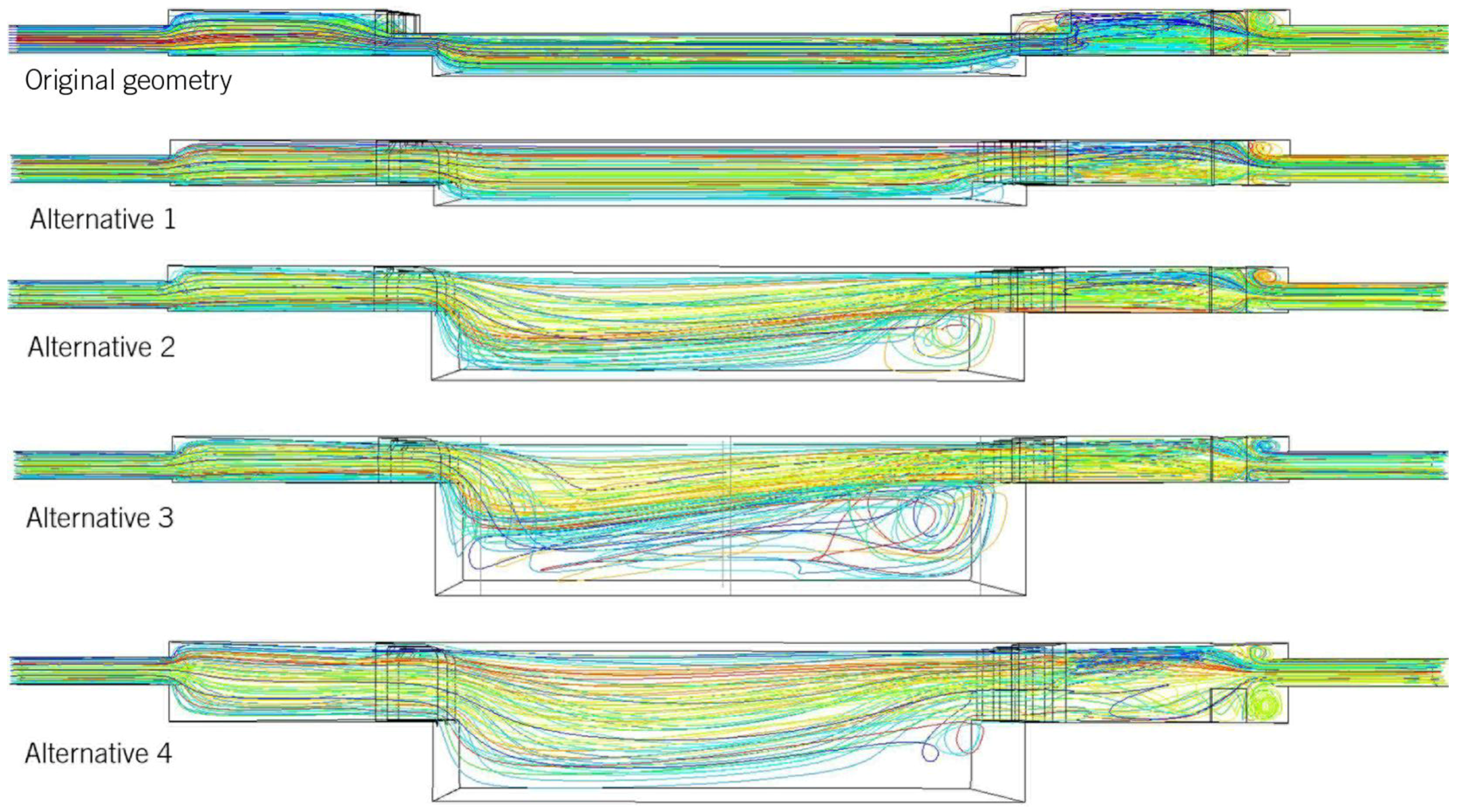
Figure 7.
Reduction in the mean module velocity as a function of the module volume for an inlet velocity of 0.1 m/s.
Figure 7.
Reduction in the mean module velocity as a function of the module volume for an inlet velocity of 0.1 m/s.
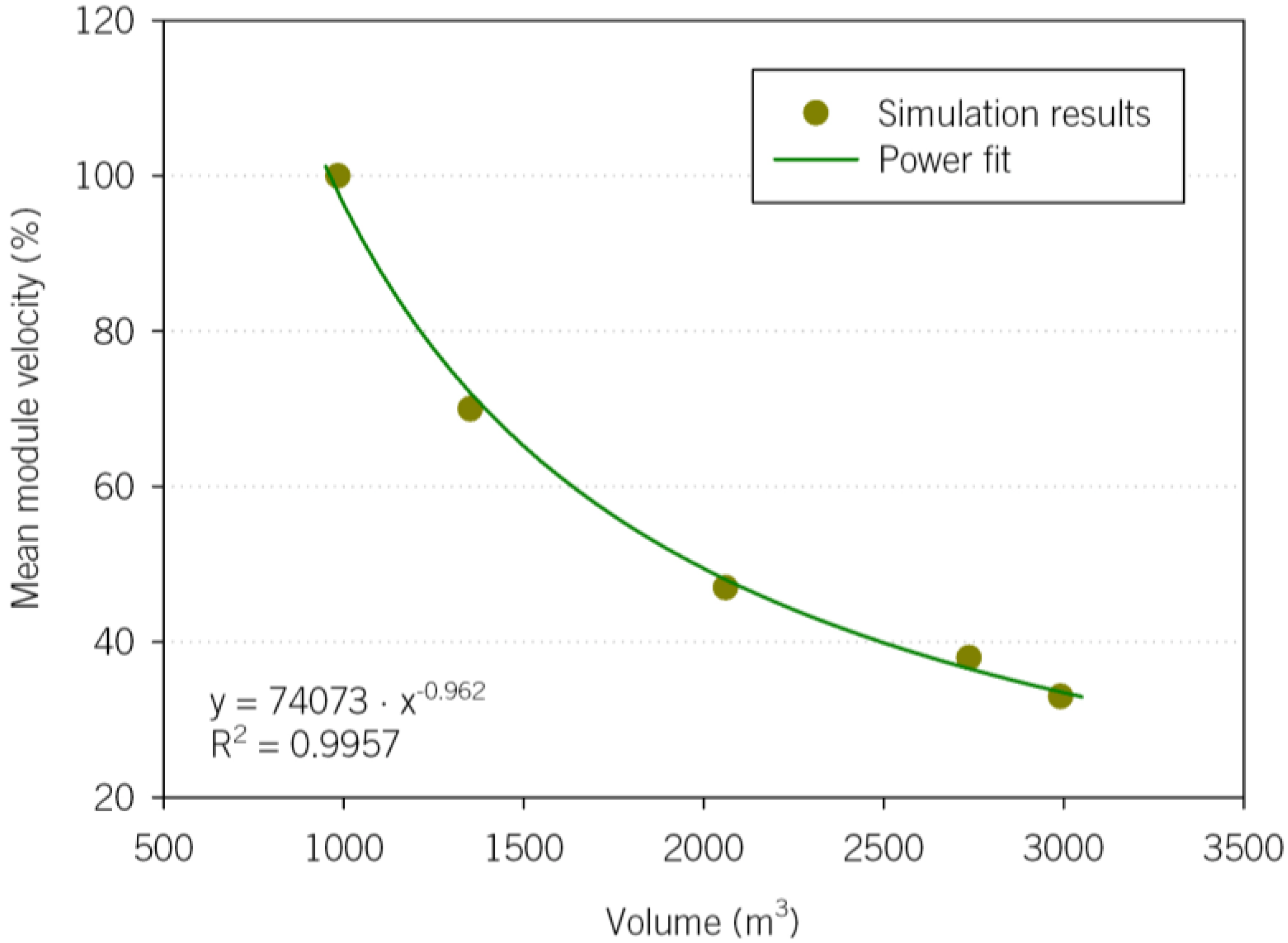
Figure 8.
Change in the velocity magnitude contours inside geometry A as function of the initial distributor design. (A) Actual design; (B) Without initial pillar; (C) Three initial pillars in triangle; (D) Two distributor rows.
Figure 8.
Change in the velocity magnitude contours inside geometry A as function of the initial distributor design. (A) Actual design; (B) Without initial pillar; (C) Three initial pillars in triangle; (D) Two distributor rows.

Figure 9.
Velocity contours for a plane parallel to the ground (z = 0.5 mm) for geometry B for different velocity inlets (A) 0.1 m/s, (B) 0.5 m/s, (C) 1.0 m/s and (D) 2.0 m/s.
Figure 9.
Velocity contours for a plane parallel to the ground (z = 0.5 mm) for geometry B for different velocity inlets (A) 0.1 m/s, (B) 0.5 m/s, (C) 1.0 m/s and (D) 2.0 m/s.

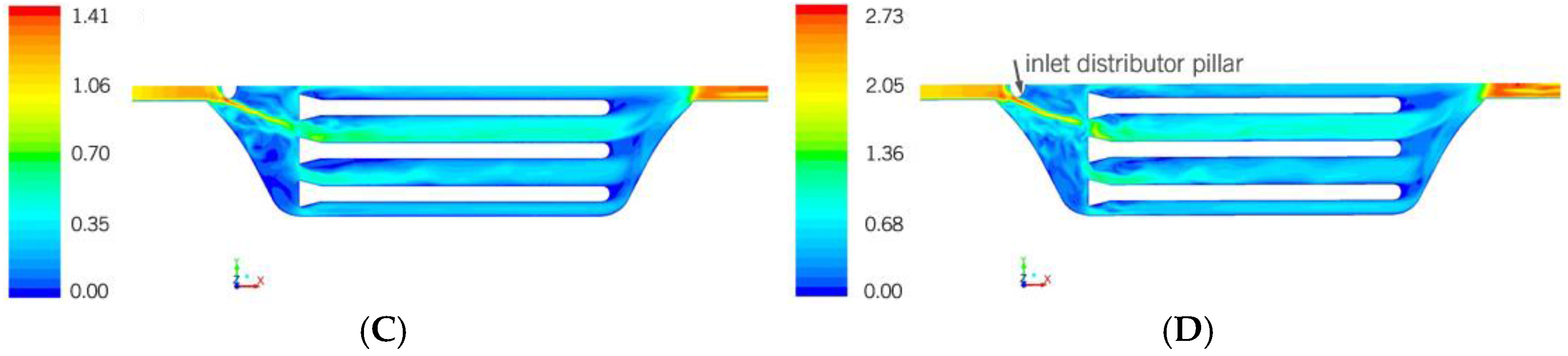
Figure 10.
Oxygen fractions at 1 s as a function of the studied parameters (red represents 100% water and blue represents 100% oxygen). The direction of the liquid is from left to right. The inlet parts without relevant information have been eliminated from the figures. The arrows in the figure indicate the gravity direction.
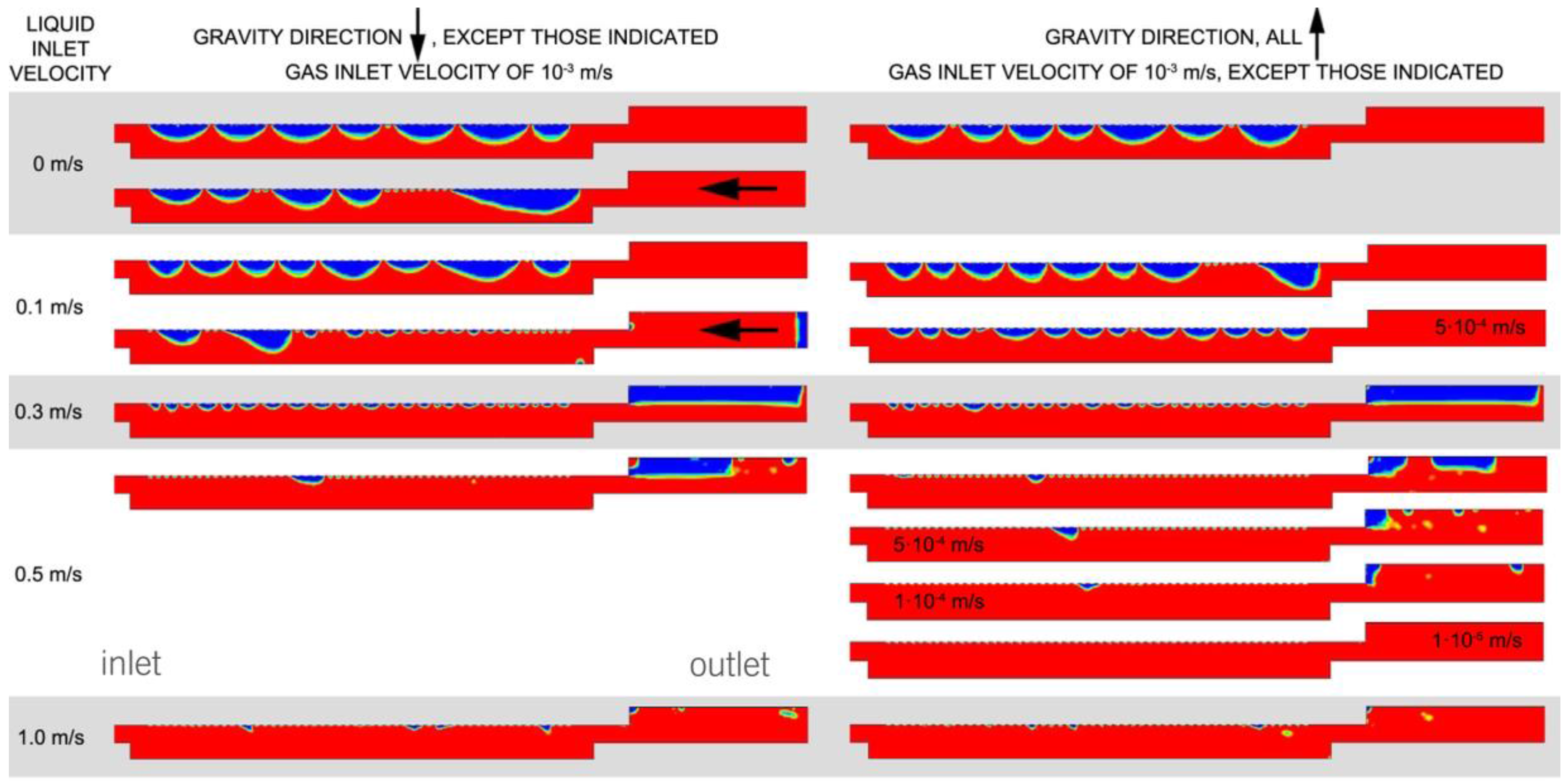
Figure 11.
Oxygen fraction for several control lines, according to Figure 3, as a function of (A) the liquid inlet velocity; (B) the gravity direction for two different liquid inlet velocities (B1: 0 m/s, B2: 0.1 m/s) and (C) the oxygen inlet velocity.
Figure 11.
Oxygen fraction for several control lines, according to Figure 3, as a function of (A) the liquid inlet velocity; (B) the gravity direction for two different liquid inlet velocities (B1: 0 m/s, B2: 0.1 m/s) and (C) the oxygen inlet velocity.
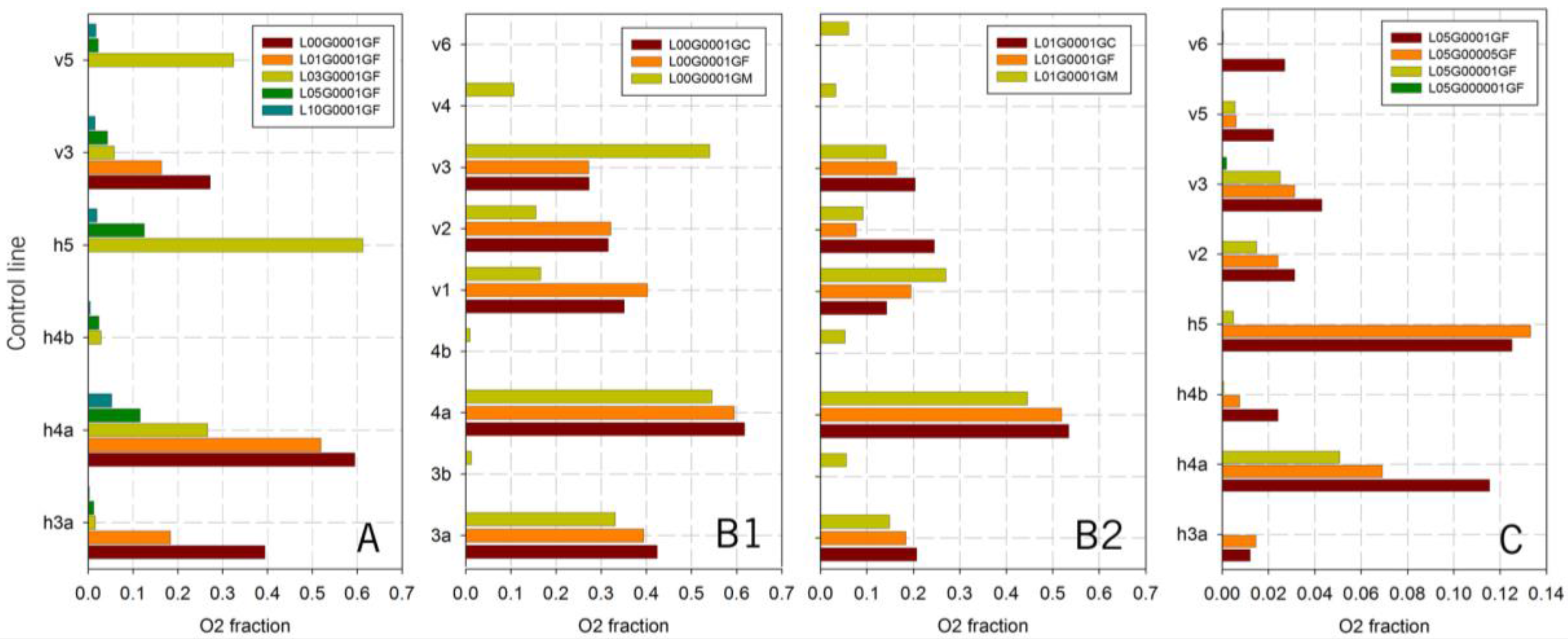
Figure 12.
Trends of the oxygen fraction as a function of the liquid inlet velocity and gravity (the gravity factor was 1.1 when the direction was against the gas inlet, GM case, and 1.0 otherwise, GC and GF cases).
Figure 12.
Trends of the oxygen fraction as a function of the liquid inlet velocity and gravity (the gravity factor was 1.1 when the direction was against the gas inlet, GM case, and 1.0 otherwise, GC and GF cases).
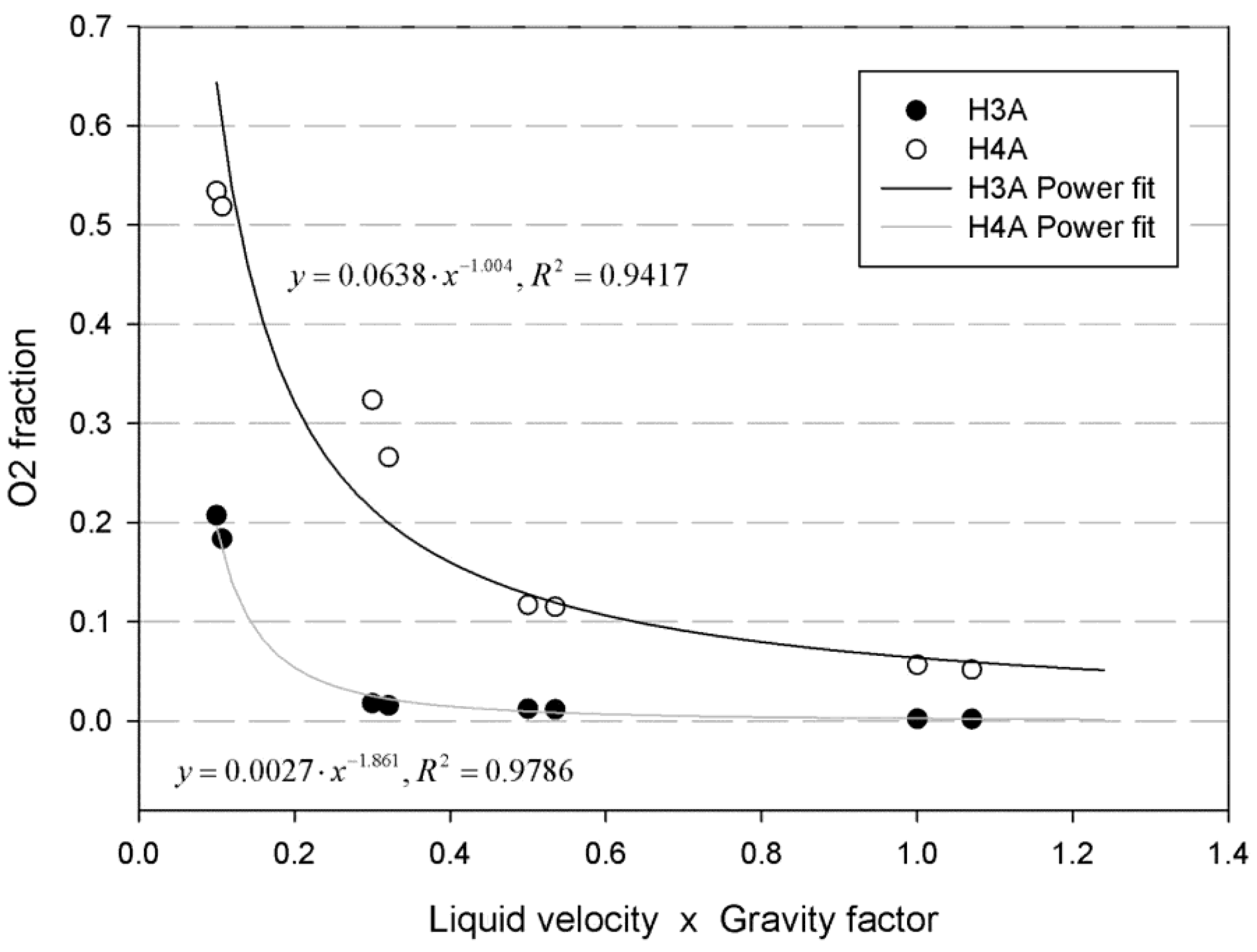
Figure 13.
Comparisons of the 2D and 3D results regarding the bubble characterization. Liquid inlet velocity of 0.5 m/s, gas inlet velocity of 0.001 m/s and GF gravity direction.
Figure 13.
Comparisons of the 2D and 3D results regarding the bubble characterization. Liquid inlet velocity of 0.5 m/s, gas inlet velocity of 0.001 m/s and GF gravity direction.
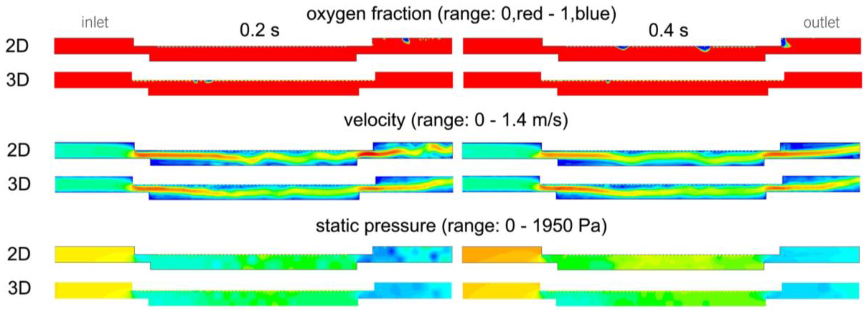
Figure 14.
Images of the experimental runs under different conditions: (A) stagnant liquid and (B) liquid inlet flow rate of 60 mL/min.
Figure 14.
Images of the experimental runs under different conditions: (A) stagnant liquid and (B) liquid inlet flow rate of 60 mL/min.


Table 1.
Liquid inlet velocity correspondences between the 2D and 3D simulations. The equivalent liquid inlet velocity corresponds to what would be the liquid inlet velocity in 3D simulations in order to have an agreement with the mean velocities inside the cell.
Table 1.
Liquid inlet velocity correspondences between the 2D and 3D simulations. The equivalent liquid inlet velocity corresponds to what would be the liquid inlet velocity in 3D simulations in order to have an agreement with the mean velocities inside the cell.
| Liquid Inlet Velocity (m/s) | Mean Velocity Inside the Cell in 2D Simulations (m/s) | Mean Velocity Inside the Cell in 3D Simulations (m/s) | Factor | Equivalent Liquid Inlet Velocity (m/s) |
|---|---|---|---|---|
| 0.1 | 0.119 | 0.012 | 10 | 1.0 |
| 0.5 | 0.544 | 0.071 | 8 | 3.8 |
| 1.0 | 1.127 | 0.160 | 7 | 7.0 |
Table 2.
Properties of the meshes used.
| Simulation Type | Elements | Nodes | Element Type | Element Quality | Skewness | |
|---|---|---|---|---|---|---|
| Geometry without channels | 3D | 731373 | 741104 | Hexahedral | 0.92 | 0.13 |
| Geometry with channels | 3D | 606418 | 600552 | Hexahedral | 0.86 | 0.22 |
| Geometry without channels (max cavity height case) | 3D | 1725495 | 306640 | Tetrahedral | 0.84 | 0.22 |
| Initial pillar study (case C) | 3D | 335188 | 368685 | Hexahedral | 0.95 | 0.03 |
| Bubble study | 2D | 12954 | 13996 | Tetrahedral | 0.85 | 0.13 |
| Bubble study 3D validation | 3D | 206663 | 43411 | Hexahedral | 0.82 | 0.25 |
Table 3.
Velocity results for different planes and for different inlet velocities—geometry A.
| Location | 0.1 m/s | 0.5 m/s | 1.0 m/s | 2.0 m/s | ||||
|---|---|---|---|---|---|---|---|---|
| Mean | Std. Dev. | Mean | Std. Dev. | Mean | Std. Dev. | Mean | Std. Dev. | |
| I1 (plane) | 0.76 × 10⁻² | 0.99 × 10⁻² | 4.90 × 10⁻² | 7.15 × 10⁻² | 13.1 × 10⁻² | 11.9 × 10⁻² | 31.0 × 10⁻² | 21.3 × 10⁻² |
| I2 (plane) | 0.72 × 10⁻² | 0.39 × 10⁻² | 4.29 × 10⁻² | 4.66 × 10⁻² | 11.0 × 10⁻² | 8.44 × 10⁻² | 16.8 × 10⁻² | 11.7 × 10⁻² |
| I3 (plane) | 0.77 × 10⁻² | 0.55 × 10⁻² | 3.66 × 10⁻² | 3.07 × 10⁻² | 7.32 × 10⁻² | 4.07 × 10⁻² | 14.7 × 10⁻² | 8.05 × 10⁻² |
| G0 (plane) | 0.67 × 10⁻² | 0.33 × 10⁻² | 3.08 × 10⁻² | 2.65 × 10⁻² | 9.29 × 10⁻² | 6.68 × 10⁻² | 18.8 × 10⁻² | 11.1 × 10⁻² |
| G1 (plane) | 1.49 × 10⁻² | 1.67 × 10⁻² | 9.78 × 10⁻² | 11.1 × 10⁻² | 20.2 × 10⁻² | 22.1 × 10⁻² | 41.2 × 10⁻² | 44.2 × 10⁻² |
| G2 (plane) | 1.75 × 10⁻² | 2.61 × 10⁻² | 10.2 × 10⁻² | 13.6 × 10⁻² | 21.1 × 10⁻² | 26.3 × 10⁻² | 42.9 × 10⁻² | 50.7 × 10⁻² |
| G3 (plane) | 1.71 × 10⁻² | 4.48 × 10⁻² | 8.69 × 10⁻² | 20.3 × 10⁻² | 18.9 × 10⁻² | 38.3 × 10⁻² | 40.0 × 10⁻² | 71.3 × 10⁻² |
| Volume | 1.28 × 10⁻² | 7.07 × 10⁻² | 15.8·10−2 | 33.7 × 10⁻² | ||||
Table 4.
Velocity results for the different planes and for the different alternative geometries of geometry A of PEC cell.
Table 4.
Velocity results for the different planes and for the different alternative geometries of geometry A of PEC cell.
| Location | A1 | A2 | A3 | A4 | ||||
|---|---|---|---|---|---|---|---|---|
| Mean | Std. Dev. | Mean | Std. Dev. | Mean | Std. Dev. | Mean | Std. Dev. | |
| I1 (plane) | 0.50 × 10⁻² | 0.76 × 10⁻² | 0.35 × 10⁻² | 0.62 × 10⁻² | 0.27 × 10⁻² | 0.54 × 10⁻² | 0.23 × 10⁻² | 0.35 × 10⁻² |
| I2 (plane) | 0.47 × 10⁻² | 0.38 × 10⁻² | 0.29 × 10⁻² | 0.38 × 10⁻² | 0.24 × 10⁻² | 0.35 × 10⁻² | 0.20 × 10⁻² | 0.21 × 10⁻² |
| I3 (plane) | 0.47 × 10⁻² | 0.26 × 10⁻² | 0.29 × 10⁻² | 0.20 × 10⁻² | 0.26 × 10⁻² | 0.18 × 10⁻² | 0.21 × 10⁻² | 0.15 × 10⁻² |
| G00 (plane) | 0.23 × 10⁻² | 0.21 × 10⁻² | 0.16 × 10⁻² | 0.13 × 10⁻² | 0.18 × 10⁻² | 0.14 × 10⁻² | ||
| G0 (plane) | 0.31 × 10⁻² | 0.21 × 10⁻² | 0.39 × 10⁻² | 0.37 × 10⁻² | 0.39 × 10⁻² | 0.37 × 10⁻² | 0.56 × 10⁻² | 0.64 × 10⁻² |
| G1 (plane) | 0.99 × 10⁻² | 1.35 × 10⁻² | 0.90 × 10⁻² | 3.09 × 10⁻² | 1.52 × 10⁻² | 3.08 × 10⁻² | 0.79 × 10⁻² | 1.34 × 10⁻² |
| G2 (plane) | 1.44 × 10⁻² | 2.48 × 10⁻² | 1.32 × 10⁻² | 2.56 × 10⁻² | 1.32 × 10⁻² | 2.57 × 10⁻² | 1.05 × 10⁻² | 2.46 × 10⁻² |
| G3 (plane) | 1.66 × 10⁻² | 3.03 × 10⁻² | 1.52 × 10⁻² | 1.39 × 10⁻² | 0.89 × 10⁻² | 1.40 × 10⁻² | 1.14 × 10⁻² | 3.00 × 10⁻² |
| G4 (plane) | 0.63 × 10⁻² | 0.98 × 10⁻² | 0.57 × 10⁻² | 1.02 × 10⁻² | 0.57 × 10⁻² | 1.01 × 10⁻² | 0.32 × 10⁻² | 0.76 × 10⁻² |
| Volume | 0.89 × 10⁻² | 0.61 × 10⁻² | 0.48 × 10⁻² | 0.42 × 10⁻² | ||||
Table 5.
Velocity results in m/s for different planes and for different inlet velocities—geometry B of PEC cell.
Table 5.
Velocity results in m/s for different planes and for different inlet velocities—geometry B of PEC cell.
| Location | 0.1 m/s | 0.5 m/s | 1 m/s | 2 m/s | ||||
|---|---|---|---|---|---|---|---|---|
| Mean | Std. Dev. | Mean | Std. Dev. | Mean | Std. Dev. | Mean | Std. Dev. | |
| I1 (plane) | 1.96 × 10⁻² | 1.27 × 10⁻² | 9.86 × 10⁻² | 8.64 × 10⁻² | 20.8 × 10⁻² | 17.3 × 10⁻² | 45.9 × 10⁻² | 36.8 × 10⁻² |
| I2 (plane) | 1.95 × 10⁻² | 1.23 × 10⁻² | 9.75 × 10⁻² | 6.57 × 10⁻² | 19.5 × 10⁻² | 12.8 × 10⁻² | 39.0 × 10⁻² | 24.1 × 10⁻² |
| I3 (plane) | 1.95 × 10⁻² | 1.16 × 10⁻² | 9.75 × 10⁻² | 6.08 × 10⁻² | 19.5 × 10⁻² | 12.8 × 10⁻² | 39.0 × 10⁻² | 24.9 × 10⁻² |
| G1 (plane) | 2.28 × 10⁻² | 1.80 × 10⁻² | 13.1 × 10⁻² | 11.3 × 10⁻² | 26.9 × 10⁻² | 23.4 × 10⁻² | 57.7 × 10⁻² | 47.8 × 10⁻² |
| G2 (plane) | 3.15 × 10⁻² | 2.41 × 10⁻² | 16.0 × 10⁻² | 12.1 × 10⁻² | 31.9 × 10⁻² | 25.4 × 10⁻² | 63.7 × 10⁻² | 48.6 × 10⁻² |
| G3 (plane) | 2.87 × 10⁻² | 4.17 × 10⁻² | 13.7 × 10⁻² | 19.2 × 10⁻² | 28.2 × 10⁻² | 36.4 × 10⁻² | 56.9 × 10⁻² | 67.9 × 10⁻² |
| Volume | 2.19 × 10⁻² | 11.4 × 10⁻² | 24.2 × 10⁻² | 51.3 × 10⁻² | ||||
Table 6.
Area-weighted average O2 gas fraction and liquid velocity in the simulated surface for the 1 s simulations for different liquid (L) and gas (G) inlet velocities and gravity (G) directions (more details in Section 2.1.2).
Table 6.
Area-weighted average O2 gas fraction and liquid velocity in the simulated surface for the 1 s simulations for different liquid (L) and gas (G) inlet velocities and gravity (G) directions (more details in Section 2.1.2).
| Case of Study | O2 Fraction | Velocity (m/s) | Case of Study | O2 Fraction | Velocity (m/s) |
|---|---|---|---|---|---|
| L00G0001GF | 0.193 | 0.038 | L03G0001GC | 0.176 | 0.314 |
| L00G0001GC | 0.197 | 0.036 | L05G0001GC | 0.085 | 0.521 |
| L00G0001GM | 0.183 | 0.049 | L05G0001GF | 0.080 | 0.530 |
| L01G00005GF | 0.129 | 0.112 | L05G00005GF | 0.044 | 0.517 |
| L01G0001GF | 0.189 | 0.124 | L05G00001GF | 0.020 | 0.559 |
| L01G0001GC | 0.202 | 0.124 | L05G000001GF | 0.003 | 0.569 |
| L01G0001GM | 0.105 | 0.116 | L10G0001GF | 0.012 | 1.122 |
| L03G0001GF | 0.168 | 0.316 | L10G0001GC | 0.019 | 1.131 |
Table 7.
Bubble characterization results. Comparison of the 2D and 3D simulation results. The results refer to area-weighted averages of the 2D surfaces and volume-weighted averages of the 3D volume.
Table 7.
Bubble characterization results. Comparison of the 2D and 3D simulation results. The results refer to area-weighted averages of the 2D surfaces and volume-weighted averages of the 3D volume.
| Parameter | Liquid Inlet Velocity: 0.5 m/s, Gas Inlet Velocity: 0.001 m/s, GF | ||
|---|---|---|---|
| 2D Case | 3D Case (Equivalent Plane to the 2D Case) | 3D Case (Mean Volume) | |
| Time: 0.2 s | |||
| Mean velocity (m/s) | 0.5308 | 0.5830 | 0.5819 |
| Mean gas fraction | 0.9810 | 0.9862 | 0.9916 |
| Mean static pressure (Pa) | 240.25 | 312.84 | 303.18 |
| Time: 0.4 s | |||
| Mean velocity (m/s) | 0.5081 | 0.5889 | 0.5798 |
| Mean gas fraction | 0.9573 | 0.9880 | 0.9928 |
| Mean static pressure (Pa) | 433.33 | 387.40 | 377.99 |
© 2017 by the authors. Licensee MDPI, Basel, Switzerland. This article is an open access article distributed under the terms and conditions of the Creative Commons Attribution (CC BY) license (http://creativecommons.org/licenses/by/4.0/).
Share and Cite
MDPI and ACS Style
Torras, C.; Lorente, E.; Hernández, S.; Russo, N.; Salvadó, J. Hydrodynamics and Oxygen Bubble Characterization of Catalytic Cells Used in Artificial Photosynthesis by Means of CFD. Fluids 2017, 2, 25. https://doi.org/10.3390/fluids2020025
AMA Style
Torras C, Lorente E, Hernández S, Russo N, Salvadó J. Hydrodynamics and Oxygen Bubble Characterization of Catalytic Cells Used in Artificial Photosynthesis by Means of CFD. Fluids. 2017; 2(2):25. https://doi.org/10.3390/fluids2020025
Chicago/Turabian StyleTorras, Carles, Esther Lorente, Simelys Hernández, Nunzio Russo, and Joan Salvadó. 2017. "Hydrodynamics and Oxygen Bubble Characterization of Catalytic Cells Used in Artificial Photosynthesis by Means of CFD" Fluids 2, no. 2: 25. https://doi.org/10.3390/fluids2020025