
Anisotropic Wave Turbulence for Reduced Hydrodynamics with Rotationally Constrained Slow Inertial Waves


1
Department of Applied Mathematics, University of Colorado, Boulder, CO 80045, USA
2
Tata Institute of Fundamental Research, Hyderabad 500075, India
Fluids 2017, 2(2), 28; https://doi.org/10.3390/fluids2020028
Submission received: 8 March 2017
/
Revised: 13 May 2017
/
Accepted: 24 May 2017
/
Published: 27 May 2017
(This article belongs to the Special Issue Advances in Hydrodynamics)
Abstract
:Kinetic equations for rapidly rotating flows are developed in this paper using multiple scales perturbation theory. The governing equations are an asymptotically reduced set of equations that are derived from the incompressible Navier-Stokes equations. These equations are applicable for rapidly rotating flow regimes and are best suited to describe anisotropic dynamics of rotating flows. The independent variables of these equations inherently reside in a helical wave basis that is the most suitable basis for inertial waves. A coupled system of equations for the two global invariants: energy and helicity, is derived by extending a simpler symmetrical system to the more general non-symmetrical helical case. This approach of deriving the kinetic equations for helicity follows naturally by exploiting the symmetries in the system and is different from the derivations presented in an earlier weak wave turbulence approach that uses multiple correlation functions to account for the asymmetry due to helicity. Stationary solutions, including Kolmogorov solutions, for the flow invariants are obtained as a scaling law of the anisotropic wave numbers. The scaling law solutions compare affirmatively with results from recent experimental and simulation data. Thus, anisotropic wave turbulence of the reduced hydrodynamic system is a weak turbulence model for strong anisotropy with a dominant cascade where the waves aid the turbulent cascade along the perpendicular modes. The waves also enable an appropriate closure of the kinetic equation through averaging of their phases.
1. Introduction
The theory of weak wave dynamics (i.e., the stochastic theory of nonlinear wave interactions) has been extensively studied since the seminal works of Kadomstev [1], Galeev et al. [2], Zakharov and Filonenko [3] and more recently reviewed by Zakharov [4], Balk [5], Choi et al. [6] and Nazarenko [7]. This theory remains one of the few areas where a mathematical framework exists with predictive capabilities for studying the energetics and dynamics associated with fluid turbulence. In this regard, the theory of weak wave turbulence was further explored in recent papers [8,9,10,11] in the context of unstratified rotating turbulent flows. The theory utilizes the incompressible Euler equation for inviscid dynamics in an infinite space, in dimensionless form:
Here is the three-dimensional velocity field in the Cartesian geometry , p is the pressure field, and is the gradient operator. Equation (1) is characterized by system rotation along with length, advective velocity, time and pressure scales denoted by and , respectively. The Rossby number , describing the relative importance of nonlinear advection to the Coriolis acceleration force, is the sole non-dimensional parameter. Of particular interest is the regime for rotationally constrained flows along with the concomitant viewpoint that the dynamics can be partitioned into fast inertial waves evolving on the rotational timescale of , and eddies evolving on the advection timescale of . In nondimensional units these timescales are denoted by and respectively. In the Cartesian coordinate system the linear inertial-wave dispersion relation, obtained from Equation (1) for Fourier plane waves with wavevector and of the form , is given by
Slow dynamics, to leading order, are geostrophically balanced, i.e.,
It follows , with and , such that pressure is now identified as the geostrophic streamfunction. On noting Equation (3) implies that geostrophic motions are horizontally non-divergent with . Moreover, such motions are columnar in nature due to the Taylor-Proudman constraint that enforces axial invariance, i.e., [12,13]. Recent work [14,15] has more precisely established this invariance as true provided , thus providing an upper bound to the degree of spatial anisotropy, i.e., .
Underlying hypotheses for the theory of rotating wave turbulence are: (i) the separation of inertial and advective timescales, i.e., and (ii) the non-interaction between geostrophically balanced and inertial waves dynamics [16]. A necessary criterion for this to occur in Equation (1) is which ensures that the nonlinear terms remain small compared to linear terms. It follows from this bound that wave amplitudes can be large outside the slow manifold. Within the regime (slow manifold), laboratory experiments [17,18] and sufficiently spatially resolved simulations [11,19,20] have clearly demonstrated the tendency for the inertial wave spectra to evolve anisotropically towards a slow manifold associated with axially invariant geostrophic dynamics (). Using wave turbulence theory on Equation (1), Galtier [8] predicts an anisotropic energy spectrum and a helicity spectrum contrary to predictions of a solution for observed in simulations [21,22]. A critical concern for this discrepancy is that the uniformity of the asymptotic approach of the weak-wave turbulence theory is lost as the slow manifold is approached. Notably, as , it is found that inertial waves still exist within the slow manifold and are slow. Such slow waves are not accounted for in weak wave turbulence literature [8,9].
Spectral power laws for anisotropic wave turbulence in the limit of rapid rotation are obtained in this manuscript. Specifically, it is found that (equivalently, and ) and are in agreement with power law solutions obtained numerically and experimentally [17,21,22,23] (see Figure 1). These solutions pertain to the slow manifold and hence differ from the power laws for the isotropic flow regime [24] and those obtained by Galtier [8,9] for the flow state outside the slow manifold. A schematic picture of the various regimes of rotating turbulence is also provided in this paper along with the respective power law solutions for each regime. This will serve in broad understanding of rotating turbulent dynamics and specifically, undergird the importance of anisotropy in the slow manifold and its influence on spectral power law solutions. It is also demonstrated that there is, in principle, a simpler approach in obtaining the coupled energy-helicity kinetic equations using the method of Hamiltonian reduction [25] and symmetries than the more algebraically tedious correlation calculations in [8,9]. For clarity and for the sake of averting any confusion, it is important to note that the derivations of the kinetic equations presented here are not the same as the derivations in [8,9]. This point is further elaborated in Section 6.4 and Section 6.5.
2. Reduced-Rotating Hydro-Dynamic Equations, R-RHD
We apply a multi-scale perturbation method directly within the slow manifold to a recently derived set of asymptotically reduced equations for rotationally constrained flows [14,1526,27]. In what follows, we adopt the nomenclature reduced rotating hydrodynamic (R-RHD) for the reduced equations describing an unstratified, non-buoyant rotating fluid. We note that R-RHD capture a slow manifold that is more precisely identified as and contains not only geostrophic columnar eddies but also anisotropic inertial waves characterized by scales: . The amplitude of these slow waves evolve on slower advective timescale.
At the outset, for convenience to aid our investigation, we centrally locate some notations and definitions involving position vector and wavenumber vector , in Appendix A.1. The detailed derivation of R-RHD is provided in [14,15]. To summarize, the asymptotic framework for Equation (1) is established by assuming the small expansion parameter and a multiple-scale expansion in the axial direction with the isotropic scale and the anisotropic columnar length scale . Fluid variables , where T denotes tranpose, are now written as an asymptotic series in terms of the small parameter, :
To leading order in Equation (1), we observe a point wise geostrophic balance: . It follows that fluid motions are horizontally non-divergent, i.e., , with where is the geostrophic stream function as in the classical theory of quasigeostrophy. The Taylor-Proudman constraint [28] associated with the geostrophic balance further requires vertical variations to be negligible on vertical scales, i.e., . Importantly, in compliance with the Taylor-Proudman constraint, the multiple scales approach permits variations of on the Z-scale [14,15]. Hereafter, in the following we set .
At the next order in Equation (1), the requisite solvability conditions, ensuring non-secular behavior of , lead to the R-RHD equations describing the evolution of unstratified slow geostrophically balanced motions:
Here , and and W are the components of the vorticity and velocity fields. Akin to classical quasigeostrophic theory, nonlinear vertical advection, , is an asymptotically subdominant process and does not appear. However, unlike quasigeostrophic theory the velocity field is isotropic in magnitude with , hence the appearance of a prognostic equation for W. Physically, the R-RHD (5) and (6) state that unbalanced vertical pressure gradients drive vertical motions that are materially advected in the horizontal, in turn, vortical stretching due to vertical gradients in W produce vortical motions. The vertical velocity, W, also generates an ageostrophic velocity fleld, , such that incompressibility, , holds to . The R-RHD remain valid provided . Consistent with the Euler Equation (1), the R-RHD also conserve, in time, the volume-averaged (over a domain B) kinetic energy and helicity :
In what follows, an investigation of wave turbulence will be applied to the R-RHD.
2.1. Geostrophic Inertial Waves and Eddies
We observe that upon linearization, the R-RHD support slow geostrophically balanced inertial waves of the form,
with planar phase function , with dimension of and can be set to 1 without loss of generality. More explicitly, the phase function can be split into two terms: , the temporal phase factor and the spatial Fourier basis. The region of validity of R-RHD is , of special interest is the limit . When this expression represents vertically invariant modes with (i.e., the 2D modes of turbulent eddies). The circularly polarized wave amplitude vector is
where denotes the handedness, ‘+’ for right-handed circularly polarized waves (with positive helicity) and ‘−’ for left-handed circularly polarized waves (with negative helicity). Here, is a complex amplitude function where . The superscript ^ represents Fourier coefficients from the Fourier series expansion of a function. In subsequent sections, we invoke the infinite box limit () and switch to Fourier transform variables thusly and (see ch. 5 and 6 in [7]). The power 2 arises from the fact that the analysis is performed in 2D, i.e., , unless otherwise specified.
2.2. Helical Basis for Circularly Polarized Inertial Waves
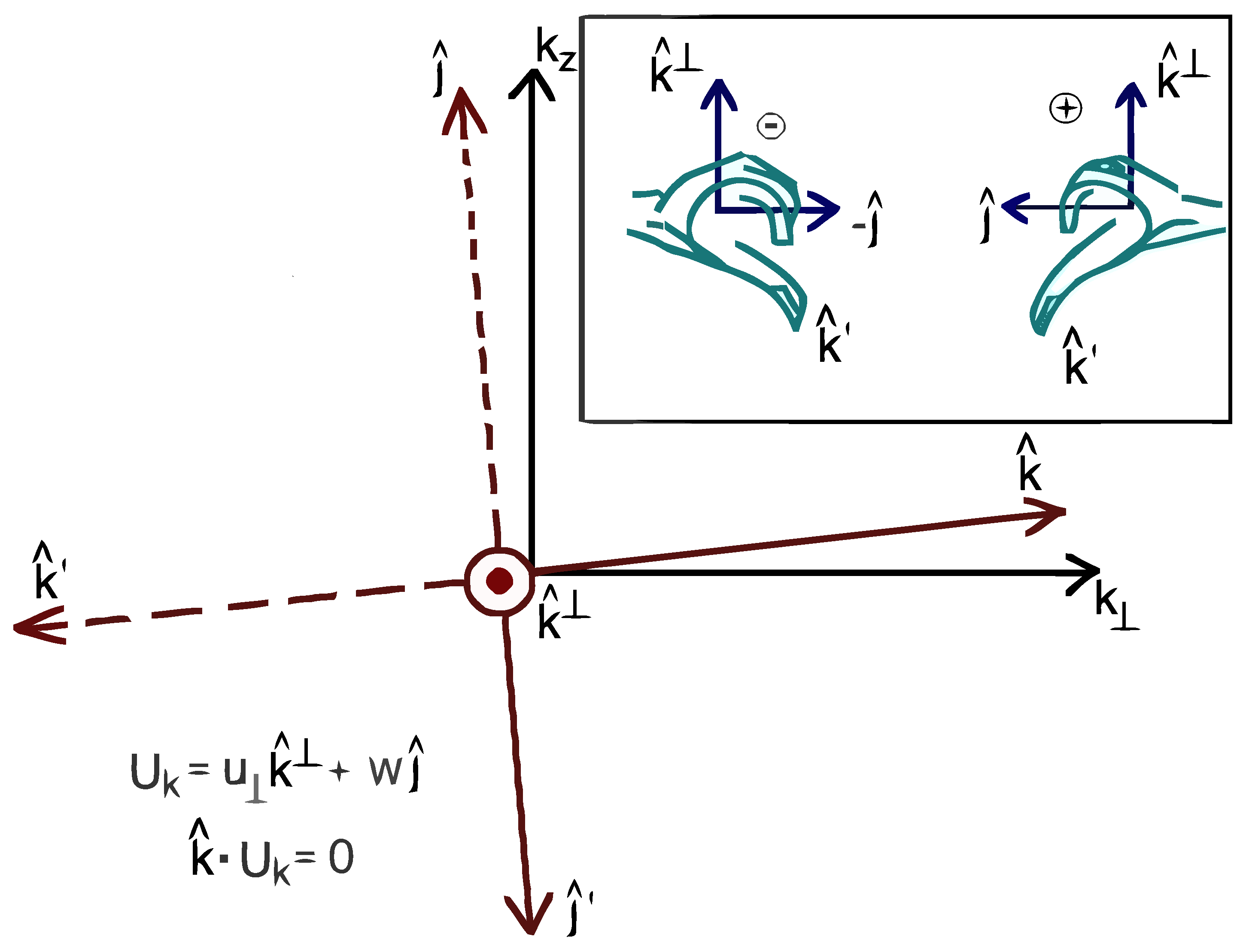
We note that in wavenumber space the unit vectors , with and , form a right-handed orthogonal basis. Within the slow manifold, we have as the direction of wave vector and henceforth we will simply call this vector (see Figure 2). The leading order velocity field associated with an inertial wave is given by
where . From (10), . Equivalently,
Here
represents the complex helical wave basis (see ref. [29] for details) within the slow manifold incorporating the leading order incompressibility criteria , i.e., . Notably, as with its counterpart that exists outside the slow manifold (ref. Figure 2), this wave basis exhibits the following property that enables switching across different handedness by a conjugation operation,
These findings illustrate that the R-RHD are naturally set up in the helical wave coordinate basis. As stated above in the paragraph following Equation (10), we switch from Fourier series to Fourier transform in the next section, i.e., e.g., unless explicitly mentioned. This switch demands a multiplication by a factor which will be explicitly written in the subsequent sections.
3. Dynamical Limits of Turbulence and Multiple Scales Order Parameters
Before we present the derivation of the amplitude and kinetic equations, a note on the time-scales of the different variables is necessary along with their order of magnitude.
3.1. Time Period of Oscillations of Waves and Amplitudes
First we introduce the scalings typically involved in weak wave turbulence [7] as applied to rotating turbulence. In terms of the time periods of oscillations, we have
where is the fast inertial wave time period proportional to as mentioned in [8] (The refers to fast waves). is the rotation rate of the system. sets the time scale for weak amplitude oscillations. Typically, and with . With these scalings, the wave time period is taken as such that . The wave kinetic equations are subsequently derived in an infinite box limit and by taking a large time limit integration as is explained in detail in [7,8,30].
The R-RHD equations introduced in the previous section eliminate the fast inertial waves with frequency but retain slow inertial waves with frequency which have the dispersion relation given in Equation (9) (The refers to slow R-RHD waves). This leads to a slight modification of Equation (14) as which we simply write below as,
where now we may have and , . We have indicating the slowness of the R-RHD waves compared with the fast inertial waves in [8]. However, for the multiple scales analysis carried forth in the subsequent sections, we adopt a new set of slow (or strained) time variables with appropriate order of magnitude as stated below.
3.2. Notations and New Slow Time Variables for the Multiple Scales Derivation Presented in This Paper
For reasons that will soon become clear, we adopt a suitable convention in our multiple scales approach by introducing new strained time variables and [31,32,33] (As an analogy, one may think of as the seconds hand on a clock, as the minutes hand on a clock and as the hour hand on a clock. The multiple scales variables and must not be conflated with the time period variables and as they have a distinct interpretation as stated here). The fast wave time scale is , the R-RHD slow waves have time scale of , while the wave amplitudes introduced in the next section have the slowest time scale denoted by . We fix our analysis by setting the most stretched time scale to order one and designate it as the slow time. In other words, we set our frame of reference to this slow time universe. Thus we have the following scale separated temporal variables:
- : slow time scale of weak amplitudes (slowest time scale),
- : slow R-RHD wave time scale, and
- : fast inertial wave time scale (filtered out by R-RHD).
Thus with , defines the magnitude of anisotropy in the flow. The R-RHD wave time derivative is . The interpretation is as provided in [31,32,33] and is articulated as follows. Note that the frame of reference is set to the most slowly elapsing dynamic denoted by . As an example, say . This means for the dynamic in the frame of reference to elapse by unit time (), the R-RHD waves would have elapsed by 100 units (i.e., ) and the fast inertial waves would have elapsed even more rapidly as seen by an observer in the set frame of reference. We conveniently have the case that within the scope of the amplitude dynamic elapsing at , the slow wave dynamic time scale is already infinitely large. However, recall that the R-RHD have filtered out the fast inertial waves by applying a method of multiple scales with as the order parameter as explained in the previous section. This means that from within the frame of reference of the reduced universe of R-RHD, the fast inertial wave is no more accessible and mathematically this means we do not need to track the dynamical universe elapsing at the time scale . This means that in our multiple scales analysis we only need to track and (we simply write t for except where we need to distinguish between and ) with
Relation (16) is equivalent to for the same choice of . So in the following we provide order of magnitude estimates for terms involving the slow inertial R-RHD waves () and the non-linear amplitude time scale () for non-linear advection in the modes. Consequently, we have representing slow (slow in comparison to the fast inertial waves that are filtered out by the R-RHD) frequency R-RHD waves with . This gives us the following limits
3.3. Definitions of Turbulence Regimes
In what follows, we will generally abbreviate reference to weak wave turbulence applied to full hydrodynamic equations by Galtier [8] as WT, anisotropic wave turbulence of the reduced hydrodynamic equations developed here, and that developed for reduced magnetohydrodynamics (MHD) [7,34], as AT, and critical balance [27] as CB. Moreover, unless otherwise stated, we will primarily refer to the works by Zakharov et al. [30] and Nazarenko [7] for the section on wave turbulence closure. The terminology anisotropic wave turbulence for reduced hydrodynamic equations is borrowed from the MHD literature [7,34] where the model was developed for reduced MHD equations [7]. This will be explained later in Section 6.2. Based on the order of magnitude scalings prescribed above, we have the following definitions.
- WT:
- .
- AT:
- . In essence, one may envision the AT dynamical regime for hydrodynamics as a zoomed in version of the WT limit in Galtier [8]. In this paper we investigate the subtle variations in the flow dynamic at this magnified scale concealed by the treatment in [8]. Further, in this paper, we perform the multiple scales analysis in the anisotropic regime defined by the order parameter . So the region of validity of AT is also set by the limit where .
- CB:
- .
As will be shown subsequently, the dynamic and solutions are distinctly different for WT and AT.
4. Wave Amplitude Equations
In the framework of this paper we consider small amplitude dynamics, where smallness of the amplitude is measured in terms of the extent of anisotropy, i.e., the ratio . However, rotating fluid motion includes significantly large wave amplitudes of outside the slow manifold. For connectivity and consistency with observed energy spectra as prescribed in this paper, one can therefore envision the scenario whereby the amplitudes of resonantly cascading inertial waves have been sufficiently attenuated once the dominant flow dynamics have reached the slow manifold. We therefore proceed with a multiple scales asymptotic approach in time, where and
where is to ensure consistency of order in the expansion above.
The order parameter is a measure of the wavefield amplitude and denotes the slow advective timescale for weak amplitude modulations in comparison to the inertial wave propagation time t. We note that , indicating that defines the advective timescale. This ensures a necessary separation of temporal scales and t as explained in [16], thereby allowing for a multi-scale treatment of the system with distinct dynamics at every order. The choice of an order parameter, proportional to has been mentioned by Nazarenko and Scheckochihin [27] and serves as a guiding principle for the theory developed here. This way a systematic multi-scale treatment that captures the anisotropy in the rotating system is developed. A multi-scale approach exploits the presence of scale separation between slow and fast dynamics. This allows the relevance of reduced models for understanding the coupling between slow-fast dynamics. The interested reader is referred to a recent paper by Abramov [35] where a reduced model for multi-scale dynamics is presented that illustrates the power of multiple scales method in a general setting.
At , the leading order solution can be interpreted as a complex field of waves undergoing resonant interactions on slow inertial timescale. At leading order, , utilizing Equation (12), we have that planar inertial waves satisfy
Here is the Hamiltonian matrix and is the identity matrix. The solution to this system is the helical base vector . It is important to note that being non-Hermitian, an extended eigen basis, including both the left and right eigenvectors, is required. This extended basis is the complex helical basis introduced earlier in Equation (12). Also of importance to the application of a solvability condition at higher asymptotic orders is the solution satisfying the adjoint problem and orthogonality condition . Given system (19), a complex wave field can now be expressed as a superposition of inertial waves and eddies (2D modes) represented in terms of the helical basis:
At , the next asymptotic order, we have for each helical mode ,
where the subscript 1 has been dropped from the right hand side of the above equations. Application of the solvability condition, , for bounded growth in , gives the wave amplitude equation in terms of the Fourier transform variables over the full space as follows:
where is the interaction coefficient. Here . The intermediary steps in the derivation of Equation (22) are given in Appendix A.2.
4.1. Dimensional Consistency of Wave Amplitude Equation (22)
For dimensional analysis, we use to represent mass, length and time. Moreover, is used as the dimensional operator, e.g., denotes the dimension of the variable W. Recall that and , is dimensionless and since we are in 2 dimensions . Thus, we have and (Here and mean the left and right hand sides of the concerned equation respectively).
For , the sum is actually carried over the combinations given by the set as the terms with have null contribution due to the resonance condition. The converse holds for . Since is real valued in the physical space, the corresponding Fourier coefficients satisfy the symmetry condition and the integration over is performed on the positive spectral space. With this physical information, we re-write Equation (22) in symmetrical form, for , as follows:
where the interaction coefficient is clearly symmetric in the second and third arguments, i.e., by noting that . Likewise, by inspection of the definition of . Hereafter, the integration over is implied. The symmetrization of the nonlinear form is discussed in detail in ch. 6 of the textbook on wave turbulence by Nazarenko [7].
4.2. Spectral Tensor
Having deduced the wave amplitude equation (23), we now proceed with the primary objective of finding the functional forms for stationary energy and helicity spectra, often referred to as Kolmogorov solutions [36]. The relation between energy and helicity in terms of the canonical complex variable, can be understood by carefully analyzing the average spectral tensor for a given spectral mode .
We review some definitions of terms at the outset. Henceforth, we use the symbol to denote the dimensional constant of dimension L. Ensemble average of the squared amplitude function enables us to estimate the energy spectral density. For a given polarity , we have
Alternatively, where the infinite box limit entails [7]. Here is the Dirac delta function and is the Kronecker delta function (In this paper, delta function written with arguments both in the superscript and subscript refers to the Kronecker delta whereas the delta function written with arguments either all in the subscript or all within parenthesis refers to the Dirac delta. In other words, is Kronecker delta whereas or refers to Dirac delta). stands for random phase and amplitude [7]. Thus we have the following relation that is valid when ,
For reference, we list the dimensions of the relevant terms again:
The average spectral tensor is defined as follows (see p. 179, Section 5.11 in [37]):
The ensemble averaging of the phase factor results in the appearance of the Kronecker delta function above. The Kronecker and Dirac delta functions may be interpreted as selector functions, i.e., and respectively. The arguments and results that follow in the rest of the paper must be interpreted in the statistical sense whereby the ensemble phase averaging can be regarded as a time averaging operation upon assuming ergodic property of the flow variables. From the relations in (25), it is clear that the following is true,
By solving the above equations, we get,
These expressions are particularly useful in the derivation of the stationary energy and helicity spectra.
5. Zero Helicity Dynamics
In this section, we analyze the special case of a flow with zero helicity, i.e., for all such that . From (25) this imposes the constraint on the complex amplitude functions where for sake of brevity we will write . This entails a reflection symmetry of the wave field and a reduction in the Hamiltonian description of the system [25] because a unique handedness, associated with one of the s variables, now describes the full system as the system described by and are mirror replicas of one another in the statistical sense. This point is explained in more detail in Sen [38]. Newell and Rumpf [39] have exploited this reduction and have studied resonance wave dynamics for the nonlinear Schrödinger’s system.
Now, the inertial waves may be interpreted as occurring in helicity couplets involving and with wavefield given by
5.1. The Hamiltonian
The interaction Hamiltonian for the R-RHD can be expressed as a power series of the complex amplitudes, , as follows:
The component denotes four-wave resonant interactions which are negligibly small and therefore not considered. Resonant self-interactions involving quadratic terms, captured by , evolve on the inertial timescale t and is already accounted for within the operator . The full Hamiltonian is in agreement with the weak wave expansion (18). The wave amplitude Equation (23) is obtained from the well known Hamilton equation
where and the three wave interaction Hamiltonian is as follows [7,30]:
5.2. Kinetic Equations
By multiplying Equation (33) with and the complex conjugate of Equation (33) with , subsequently subtracting the latter from the former, followed by ensemble averaging and using the results from Section 4.2, we obtain an evolution equation for :
where and as stated earlier. Henceforth, we simply write for . Here, refers to imaginary part of the argument in parenthesis. The triple correlation can be defined as follows:
where the is a convenient way of writing the Dirac delta function . On evaluating the ensemble average and considering the infinite box limit, we have the following reduction:
Here is the Kronecker delta function that takes the value 1 when and 0 otherwise. The relation (36) implies . Then Equation (34) can be written as
Here we have simply written and hereafter the will be implied unless otherwise mentioned. We observe that Equation (37) is not closed in the sense that the left hand side of the equation is a second order correlation function that is expressed in terms of third order correlation functions on the right hand side. For Gaussian distributed fields, odd correlators are null. Hence, we must devise an estimate of using a property of the fourth order correlator for Gaussian statistics as described in the following section.
5.2.1. Closure
In order to close Equation (37), we need to express the triple correlator in terms of second order correlators. Note that Equation (37) is obtained at as explained in Section 4. An estimate of the triple correlator in terms of the second order correlator can be obtained at the previous order of the multiple scales perturbation, i.e., at , as explained in this section. On applying Wick’s theorem to the Gaussian distributed wave field, quadruple correlation functions are defined as follows [7,30]:
The applicability of Wick’s theorem relies on the assumption that the field is Gaussian distributed and this point is further discussed in Section 6.5. Let us first recall some relevant order of magnitude for the terms involved in this section. Since , we take where such that . Also, with implies (The total derivative is given by and since , we have ). We use the definition of in (35) and Equation (33) to write a differential equation for . The solution of this differential equation provides us an estimate of at to close the Equation (37) that was derived at .
The ensemble average of the phase factor can be succinctly captured by the Kronecker delta (This can be readily checked by assuming ergodicity and computing the ensemble average as a large time average), which is equal to at the infinite box limit, . Thus at , for the triadic wave process, we have
The second equality follows from the following calculation. Applying the product rule of differentiation, we have . The first term on the r.h.s. is calculated as follows:
![Fluids 02 00028 i001]()
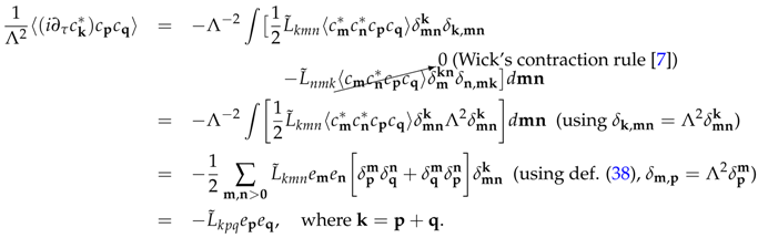
Here, the integral is expressed as a sum to make the calculation explicitly clear for the reader. Note that dimensional consistency demands where appears here because of the relation in the def. (38). Similarly, and with . Thus follows the second equality in Equation (40).
The r.h.s. of Equaiton (40) is independent of time because we are interested in stationary solutions. The solution to the differential Equation (40) is
By taking the limit for , we have the average of the exponential term approach zero because when . Thus in the long time limit, the estimated average is expressed as follows:
Thus, we have a reasonable estimate for in Equation (37) that is obtained as above at . Recall that the solutions described in Section 4 are the slow R-RHD waves that enable this closure procedure. We now plug in this estimate for in Equation (37) to close the kinetic system. The occurrence of the singularity () is averted by circumventing the pole by adding a small term to the denominator. Then we use the identity: (For a function that is analytic on the upper half of the complex plane, , where P refers to the principal value. For the special case when , the preceding identity is concisely written as where it is generally understood that the integral is taken over the domain with . The imaginary part of the l.h.s., thus, yields the delta function term on the r.h.s. of the identity) and substitute the resulting term for in Equation (37) to obtain the closed form of the kinetic equation:
5.2.2. Dimensional Consistency of the kinetic Equation (43)
5.2.3. Physical Realizability of Spectrum Prescribed by Equation (43) and Comparison with Quasi-Normal Type Closures
Quasi-Normal family of closures (including modified versions like EDQNM) are well known statistical closures which are widely used in analytical study of turbulence [41,42,43,44]. However, as pointed out by Orszag [42], the original Quasi-Normal closure results in an unphysical negative energy spectrum. This issue was shown to be related to the presence of time-history integrals in the evolution equation of the correlation function. This was corrected in modified versions of the closure, such as Quasi-Normal Markovian and Eddy Damped Quasi-Normal Markovian (EDQNM) closures [37,42,45]. EDQNM is widely used in turbulence predictions and works well in the absence of waves [46]. However, as shown by Bowman et al. [46], Bowman and Krommes [47] and noted in [48,49], in the presence of waves, especially Rossby, inertial and drift waves, EDQNM is unphysical in the sense that the energy spectrum, obtained by performing the closure, becomes negative for dynamically important Fourier modes (see Figure 1 and Figure 2 in [46] and Figure 1 in [47]). This unphysical energy condition, in the presence of waves or mode coupling, is shown to stem from the violation of the realizability criterion . This is because of the application of the fluctuation-dissipation ansatz that must be invoked in order to capture the two time correlation information within a single parameter, the triad interaction time [50]. Conceptually, this loss of realizability can be checked for a test case by assuming the total damping coefficient to be constant in time but complex valued (e.g., purely imaginary), whence can be shown to be oscillatory about zero. In fact, Bowman [50] explicitly shows that the realizability condition is violated for an actual stochastic problem involving three-wave interactions (see ch. III in [50] for details). As a remedy, a realizable Markovian closure was proposed by Bowman et al. [46], Bowman and Krommes [47], Bowman [50].
In contrast, in this paper, a wave turbulence closure [7,30] is used as explained in Section 5.2.1. In this context, it is essential to check the physical realizability of the energy spectrum permitted by the kinetic system derived above. Following the strategy prescribed by Orszag [42] (cf. p. 313, ch. IV), we envision a scenario where, starting with a positive initial condition for the energy spectrum, we assume
Here ∀ should be read as for all. The above assumptions mean that physically we have a situation where the energy in a certain mode is null at time . Specifically, note that and at . The goal is to investigate if the energy becomes negative for this specific wave mode at times . By inspection, it is clear that
because and the fact that the terms in the square parentheses are positive. The above inequality is obtained by substituting in the r.h.s. of Equation (43) when evaluated at time . This means that the mode with null energy receives energy from the interacting modes of the triad and the energy of that mode becomes positive, i.e., the nonlinear transfer to the mode is positive and energy is dumped into this mode. The above argument can be extended to any wave mode and for all times in a straight forward manner. Thus, the spectrum prescribed by Equation (43), and obtained by the wave turbulence closure described in the previous section, is non-negative and physically realizable. This can be attributed to the absence of any time-history integrals in Equation (43). In fact, the separation of time scales, captured by relation (15), enables us to take the long time limit and thereby time dependent oscillatory terms are eliminated as shown in the short paragraph following Equation (41). It is essential to note that the above inequality does not comport with the stationary state of the spectrum for the obvious reason that the derivative is non-zero. So the spectrum eventually adjusts itself to the stationary state permitted by the kinetic system derived earlier and for which the power law solutions are given in a subsequent section.
5.2.4. Invariants of the Closed Kinetic Equations
It can be shown easily that the total interaction energy given by Equation (43) is conserved, i.e., using the result of Appendix A.3. The proof in the appendix is essentially a statement of conservation of energy in each wave triad. The form of the interaction coefficient ensures the convergence of the collision integral appearing on the r.h.s. of Equation (43), thereby it meets the first criteria for the realizability of a Kolmogorov spectrum, i.e., stationary energy spectrum solution to (43) [36]. This point is elaborated in Section 5.2.6.
5.2.5. Kolmogorov Solution of the Kinetic Equations
The exact steady state solution of the kinetic Equation (43), as power laws, is obtained by assuming locality of the scale-by-scale energy transfer. This is illustrated in Nazarenko [7], Zakharov et al. [30] and earlier papers referenced therein.
Owing to the constrain imposed by the AT limit , the turbulence cascade under investigation is in the direction and (i.e., is within a relatively small r vicinity of ) serves as a tracking parameter to ensure that we do not violate the condition: . The four possible stationary solutions for the anisotropic spectrum, , are listed as follows [7,30]:
- (i)
- and (Rayleigh-Jeans (RJ) spectrum).
- (ii)
- and .
- (iii)
- and , where and are respectively the powers of and in . Clearly, in our case, . Thus, and .
- (iv)
- and . This solution corresponds to the constant flux in the z-component of the momentum.
Solution (iii), above, corresponds to the only constant energy flux solution, a necessary requirement of Kolmogorov’s theory and of primary concern in this paper. The constancy of energy flux can be easily verified by noting that ; whereby on integrating with respect to and demanding constant energy flux in the perpendicular direction, we can extract the aforementioned solution. Here, denotes the flux of energy. The direction of the flux can be ascertained by comparing the power law solutions of the RJ spectrum with that of the constant energy flux solution, i.e., since , the energy cascade is direct and the energy flux is towards smaller scales ( p. 139 in ref. [7]). Thus, the exact solution for the Kolmogorov-Zakharov-Kuznetsov spectra with constant energy flux is as follows:
This result is in agreement with experimental and computational simulations [17,22,23]. Additionally, LaCasce [51] has discussed the observation of a spectrum in the context of barotropic vorticity model using data obtained from several numerical simulations. Moreover, since converges for the spectrum (45), the Kolmogorov spectrum obtained above has finite capacity [7]. The limit is further discussed in the next section.
5.2.6. Locality of Interactions and Convergence of Collision Integral
As stated in the previous section, the Kolmogorov solutions obtained above are based on the assumption of locality of interactions. To validate the applicability of the locality assumption, it is sufficient to comment on the convergence of the collision integral on the r.h.s. of Equation (43) for the concerned power law solution [7,30,36]. However, analyzing the convergence of the collision integral is a delicate task [52] and a rigorous commentary is not within the scope of this paper. However, in this section, we will argue on the convergence of the collision integral given by the r.h.s. of Equation (43) based on inspection of the terms in the integrand, the surface over which the integration is performed and numerical integration of the same within the region of validity of the AT limit of R-RHD.
The integral in Equation (43) is in six dimensions, viz., if we further consider the decomposition of the perpendicular modes, . We have four delta functions, viz., three over the wave numbers and one over the frequency. Integrating over each delta function reduces the dimension of integration by one. So by substituting in the respective integrands, we can completely eliminate integration over the three wave numbers. Consequently, re-writing the frequency resonance condition in terms of the substituted expressions for and , we finally have a surface integral over and dimensions where the surface is defined by . This is illustrated concisely as follows.
Here defines the surface over which the integration is carried out when the collision integral is projected on the plane. Interestingly, and conveniently, the surface of integration turns out to be identical for both the first and second integrands when projected on the plane. By inspection, the surface S is singular at and . Clearly, is outside the validity of AT because we must have , so we must not be concerned about the pole at . The second condition requires more careful inspection. It defines the equation of a plane in the coordinates because it can be expressed as
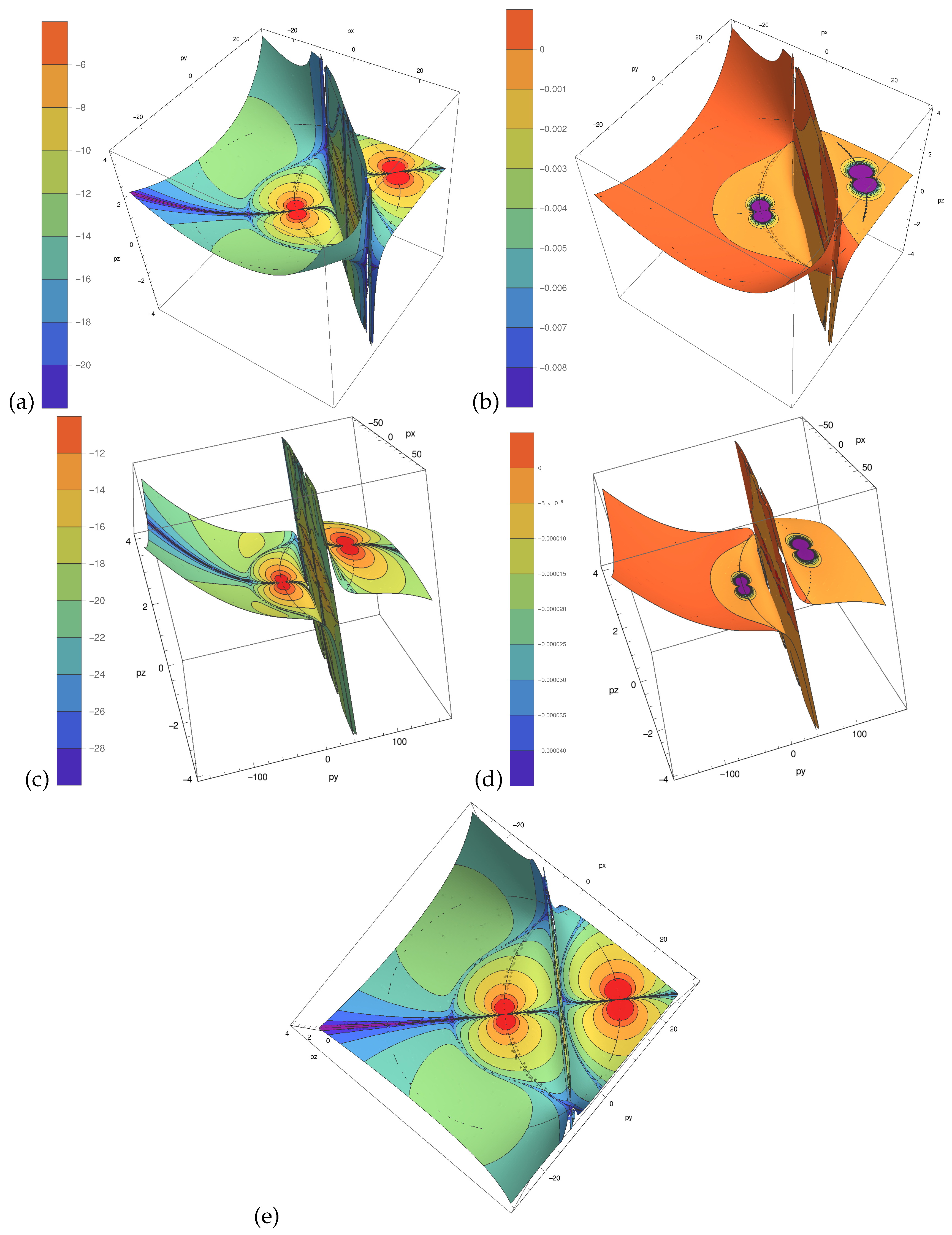
Figure 3 illustrates this singular plane on the surface S for two distinct limiting wavenumber configurations: and ( is just the opposite case). Equation (47) can also be re-written as follows,
This implies that for the first integral corresponding to the collision integral in Equation (43), we have because of , whence we have and thereby . Similarly for the second integral we have because of from which we have and thereby . This means that the integrand is identically zero on the singular plane on S and hence the integration along this singularity may be safely circumvented without blow up. Similarly, averting demands (always true) and . The latter condition is ensured because when based on very similar arguments as mentioned above.
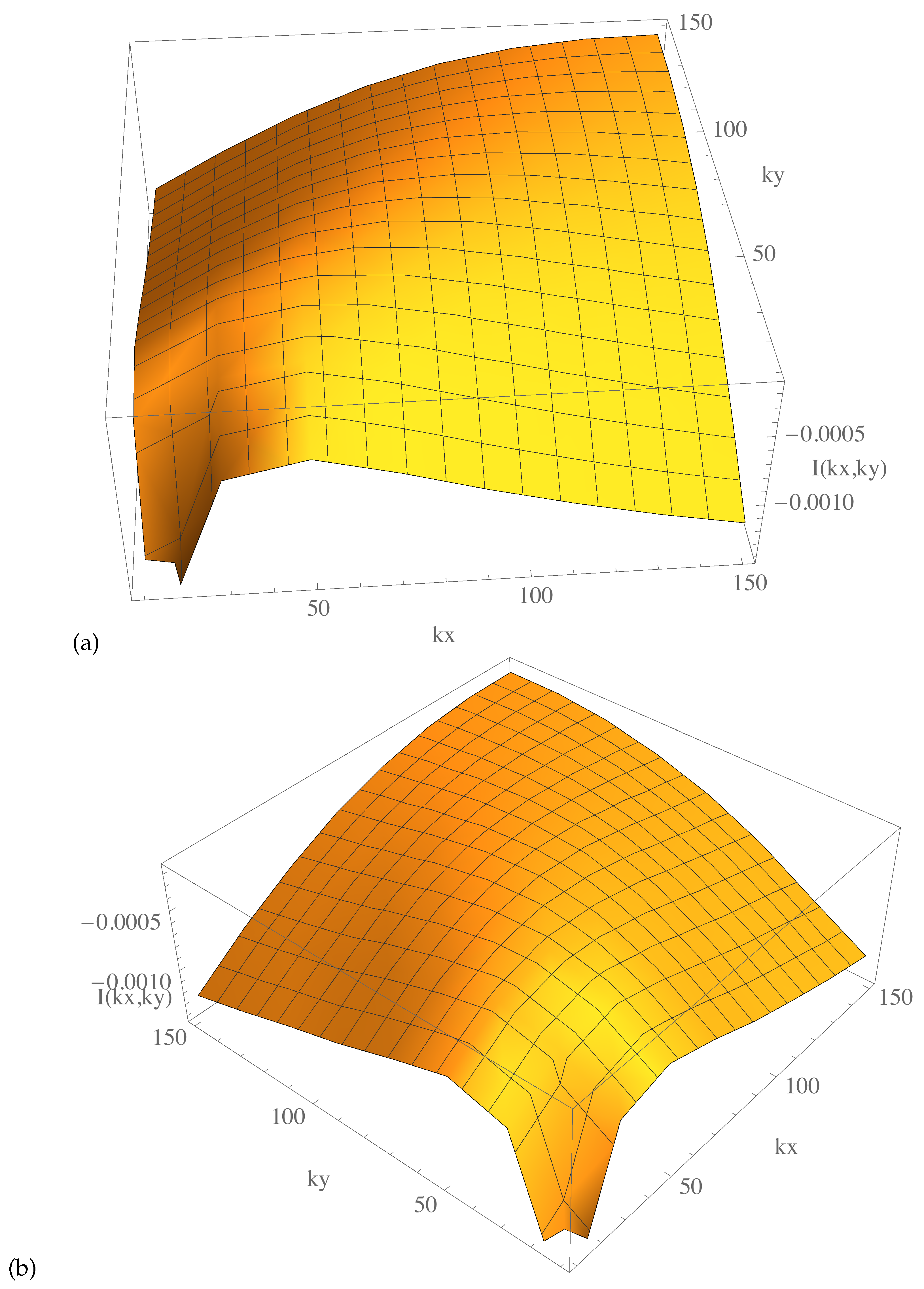
There are two other regions in Figure 3 that stand out for inspection, viz., and for the value of the integrand is high at these points due to the large values of and . These correspond to and respectively and for reasons discussed above are outside the region of validity of AT (R-RHD). Hence these points do not contribute to the integral. In general, the anisotropic limit ensures that the region of integration is typically farther away from the singular plane defined by (47) where the value of the integrand is diminishingly small as can be seen from the contour plots in Figure 3. So we know at the very least that we are safe in terms of blow up of the integrand. However, we must still investigate whether or not the accumulation of these small values of the integrand increase in an unbounded fashion over a reasonably large radial wavenumber in the plane. In order to check this we resort to numerical evaluation of the collision integral (The singular points are carefully excluded for they are found to be inconsequential as discussed above) for a range of perpendicular wave numbers. The general form of the collision integral in the kinetic Equation (43) upon projection on the plane is
The analytic expression for the Jacobian term is too messy to be written explicitly here but can be inspected symbolically using the computer program attached in the Appendix A.5. Most importantly, this term shares the location of the poles with that of the surface . Hence no additional caution is required for this term. Since we are interested in analyzing the convergence of this integral, we have ignored the constant multiplier on the r.h.s. of Equation (43). We numerically integrate the function (the integrand in expression (50)) over the surface S defined by Equation (46) by two different methods, viz., adaptive quadrature method and adaptive Monte Carlo method. The numerical integration is performed over S by excluding the singular points described in the previous paragraph as the singularities were either outside the region of validity of AT (R-RHD), i.e., outside the region where is true or occurred at points where the integrand is identically zero. The computer program used to generate the plots in this section is given in Appendix A.5. By analyzing Figure 4, it is evident that by staying within the region of validity of AT (R-RHD), as has been elaborated above in this section, the collision integral is convergent. Moreover, it is clear from the results of the numerical integration that the convergence holds for reasonably large values of thereby permitting an energy cascade to develop. Figure 4 shows that the collision integral on the plane plateaus away from the boundary of integration (at the boundary, the numerical integration is less accurate) and is very nearly zero as is expected for a stationary solution.
In this section, we have provided direct evidence of the convergence of the collision integral by numerical computation to validate the applicability of the locality assumption for seeking the Kolmogorov constant energy flux solution. For a rigorous analysis of convergence of collision integrals in a three wave system, one may refer to the work by Connaughton [52]. Additionally, it is important to note that analysis of stability and evolutionary non-locality of concerned spectra subject to extra perturbative forcing in this anisotropic limit is beyond the scope of the current paper and the interested reader is referred to the work of Balk and Nazarenko [36] and Nazarenko [7] for details.
6. Non-Zero Helicity Dynamics: Interplay of Energy and Helicity
In this section, we deduce a general set of coupled equations for the two invariants of the flow. This is done by formally extending the symmetrical system of the previous section.
6.1. Coupled Equations for Energy and Helicity
Recall that the assumption, implies , i.e., . However, on relaxing such an assumption, a coupled set of equations for energy and helicity may be arrived at by using Equation (28) in Equation (43) (cf. in Equation (43) is actually ). Thus the closed form coupled energy-helicity equation becomes,
The individual evolution equation for (and ) follows by adding (and subtracting) the two set of equations expressed concisely by Equation (50) and is given as follows:
and
Equations (51) and (52) clearly reveal the coupled dynamics of energy and helicity in a rapidly rotating fluid flow. The possibility of recovering the total energy and helicity spectrum from the simpler zero helicity case relies on extending the functional on the right hand side of Equation (43) to the non-zero helicity case.
In essence, we have taken a special case of the kinetic equations which has the functional form (think of as the right hand side of Equation (43)) where , and extended it to the more general case where . In this general case, the domain of is still the positive real line because the inequality implies that and are not independent variables and is always true. Hence, we have extended the applicability of the kinetic equation from the simpler symmetric case (where because ) to the more general case with non-trivial helicity. This way we have circumvented tedious algebraic computations involving multiple correlation functions (to account for the departure in mirror symmetry in the fully helical case) by first, reducing the Hamiltonian system by invoking reflection symmetry and then formally extending the symmetrical system to the more general helical case. The applicability and implication of this procedure is explained in more details in [38].
6.2. Generalized Solution of Energy and Helicity Spectra
Note that Equation (28) are consistent with the definitions, and . Clearly, the power law solutions do not change for the non-zero helicity case because the homogeneity of the interaction coefficient and the linear dispersion relation remains the same. Thus, for . Dimensional analysis implies, that is consistent with earlier findings based on numerical simulations [21]. The cylindrically symmetric solutions are:
The power law solution obtained here pertains to the perpendicular cascade within the slow manifold, the reader is referred to Bellet et al. [53] for power law solutions of the spectrum in the axial direction. It is important to note that the solutions given by Equation (53) are different from the ones discussed in Pouquet and Mininni [24] as the latter assume isotropy in their arguments to show that the sum of the powers of the wave numbers for and is equal to 4. The solution set of Galtier [8] belongs to the regime where the effect of fast inertial waves is dominant. In the recent work of Galtier [9], it has been shown that within the theory developed in the earlier work of Galtier [8], the power law solutions can be generalized to the empirical form presented in [24]. In contrast, the analysis presented here captures the dynamics in the slow manifold where the flow is highly anisotropic and the effect of the fast inertial waves is sub-dominant, and accounts for a distinct separation of temporal scales, t and as is necessary [16] and explained in the introductory section here. In such a regime in the slow manifold that is devoid of fast inertial wave modulation and where the dynamic is well captured by the R-RHD equations, the stationary power law solutions, that are entirely dependent on the functional form of the interaction term and the dispersion relation , are given by Equation (53) and is in agreement with results from numerical simulations (e.g., the work of Mininni and Pouquet [21], Teitelbaum and Mininni [22]). It may be interesting to point out here that an identical spectrum for has been reported in the case of anisotropic MHD turbulence of Alfven waves in the presence of strong external magnetic field (where dominant modes are ) [7,34,54]. The analytical results for the anisotropic MHD case were developed based on the reduced MHD model referenced in [7]. Thus it may not be surprising to draw an analogy between the anisotropic MHD wave turbulence and the anisotropic hydrodynamic case discussed in the current paper where the strong magnetic field plays the role of rapid rotation, and the polarized Alfven waves are congruent to the helical inertial waves discussed here (please see the Table 1 in Appendix A.4).
The important point to note here is that rotating turbulence encompasses several different and distinct dynamical regimes, each with distinct set of solutions. Hence, the importance of using reduced equations for distinct asymptotic limits as has been explained by Nazarenko and Scheckochihin [27] (see Appendix A of [27]). Within such a distinct limit of rapid rotation, the R-RHD equations have been derived [14,15,26,27] and a multiple scales perturbation method has been applied in this paper for the asymptotically reduced equations. In the following sections, we attempt to stitch together the important results of weak and strong turbulence of different dynamical regimes in order to clarify the picture of turbulent cascade that has evolved based on recent research literature.
6.3. Hierarchy of Slow Manifolds in Anisotropic Wave Turbulence Diverges from the Critical Balance Route towards Isotropy
The discussion in this section is motivated by the turbulence cascade picture presented by Nazarenko and Scheckochihin [27]. We modify the turbulent cascade schematic based on the results presented here.
The critical balance with polarization alignment argument presented by Nazarenko and Scheckochihin [27] is an attempt to explain the energy spectra observed in several numerical simulations of rotating turbulence [17,21,22,55]. However, as is evident from Figure 5 and the corresponding sketch in [27], the critical balance with polarization alignment leads to a departure from anisotropy and is a path to the recovery of isotropic scales that are prevalent above the Zeeman wavenumber [23]. It must be emphasized that anisotropy is dominant in rotating turbulent flows. It is in this light, we believe that the energy spectra is obtained for anisotropic wave turbulence in the regime of R-RHD defined by AT ( and ). In this anisotropic regime, the slow inertial wave frequency is much smaller than the fast inertial wave frequency. This solution prevails as the flow traverses a hierarchy of slow manifold regions with successively decreasing and is the anisotropic wave turbulence solution for the energy spectra within the slow manifold. In summary, there seems to be a bifurcation of the energy spectral solution at the critical balance wavenumber (see Figure 5), two distinct spectra evolve, each with a energy spectra: one leading towards the isotropic scale via critical balance and hence falls within the realm of strong turbulence (Strong wave turbulence is fairly complicated (see secs. 3.2 and 14.6 in [7]) because the wave amplitudes can be or higher [56] and the perturbative expansion may not be readily possible. Its description is incomplete as stated by Nazarenko [7]), and the other towards highly anisotropic horizontal scales with sustained by small amplitude resonating wave modes.
6.4. Comparison with Weak Turbulence Theory of Galtier
In this section, we contrast the theory presented here with earlier works [8,9]. The main distinctive features are listed below.
- The governing equations on which the wave turbulence theory [8,9] is developed are the Navier-Stokes equations (i.e., Equation (1)). In these equations, the Rossby number appears explicitly and is used as an order parameter in the perturbation analysis and the fast inertial wave dynamic is dominant. In contrast, the governing equations for the analysis presented here are the R-RHD (i.e., Equations (5) and (6)). The asymptotic limit of infinitesimally small is already accounted for in the multiple scales analysis to derive the R-RHD and hence do not explicitly appear in the R-RHD equations. This means that the effect of fast inertial waves is sub-dominant here and the R-RHD equations are hence suitably applicable for the slow manifold dynamics.
- The dynamical regime where the theory [8,9] is valid is . This point has been elaborated in great detail in the work of Nazarenko and Scheckochihin [27] (see Section 2 in [27]). The dynamical regime of the R-RHD is and . It is the limit in which is so small that the turbulent dynamic is populated by slow inertial waves with dispersion relation embodying slow oscillations when (also see Figure 5 above). In other words, within the slow manifold, is so small that . The perturbative analysis presented here is applied to the R-RHD where the smallness (weakness) of the wave amplitude is measured by and the slow dispersive three wave system undergoes weak non-linear exchanges at the asymptotic order as explained earlier in Section 4 and Section 5.
- In wave turbulence theory of Galtier [8] and Galtier [9], the kinetic equations for energy and helicity are derived by using multiple correlation functions to capture the energetics as well as the absence of symmetry due to helicity. This makes the calculations tediously lengthy. In contrast, the derivation for the helicity kinetic equation is presented here as a natural extension of the symmetrical non-helical system and bypasses the use of calculations using multiple correlation functions. This simpler approach follows a more general philosophy of Hamiltonian reduction exploiting symmetries in the system [25] and their natural extension to understanding asymmetrical phenomena.
- Finally, the spectral power laws obtained for the energy cascade are distinctly different as explained concisely in Figure 5.
Despite the fundamental differences in the region of validity of the two theories, they present a more detailed recipe to better understand turbulent energetics and cascades for rotating flows. A simple schematic towards this goal is presented in Figure 5 above to highlight the key findings in this field.
6.5. Comparison with Weak Turbulence Theory of Newell: Cumulant Hierarchy vs. Wave Amplitude Hierarchy
The fundamental difference between the multiple scales perturbation technique employed in this paper to derive the kinetic equations and the weak wave turbulence theory reviewed by Newell et. al [39] is explained in the following paragraphs.
Weak turbulence calculations, as reviewed by Newell et. al. [39], are computed by taking the closure in the limit . The third and higher order cumulants survive at the advective timescale () in the presence of fast inertial waves. This implies prevalence of non-Gaussian statistics. This is the reason for writing a hierarchal system for the cumulants in the perturbation approach, cf. Newell et. al. [39], rather than for the Fourier amplitudes.
The dynamics explained here elapse at the much slower advective time scale () compared to the faster wave timescale . At this slower time scale, it is assumed that the third (and higher odd) order cumulants are sub-dominant thereby corroborating the suitability of Gaussian statistics for the wave field. This aspect is detailed by Nazarenko [7] (see p. 64 in Section 5.6). This justifies the applicability of Wick’s theorem in the derivation of the kinetic equations. Consequently, this is also why we employed a hierarchal expansion for the wave amplitude in Equation (18).
7. Coupling between Wave and 2D Modes Through Non-Resonant Interactions
Neither the theory presented in [8] nor the model presented in this manuscript address the issue about the possibility of wave modes pumping the 2D modes. Note that when because of the fact that . Thus, within the framework of purely resonating wave triads, it is not possible to establish the coupling between wave and purely 2D modes. This should not be surprising because the theory developed is that of dispersive waves that are in resonance. However, a rather phenomenological explanation may be insightful for explaining the coupling between wave and 2D modes, as is presented below.
Suppose that in Equation (22), the triadic resonance condition is modified such that . This condition represents non-resonant (or near-resonant) interaction of the three wave modes. For small , Taylor expansion implies,
i.e.,
Thus computing the fast time integral after Taylor-expanding the exponential term reveals that the higher order slow secular terms (cf. presence of in the higher order terms) are inherently embedded in the full system that is not restricted to resonating triadic wave interactions only. These terms account for the coupling with the 2D modes. This is evident by re-writing Equation (22) with the higher order terms as follows,
The slow secular behavior of the non-resonant term (after integration) can be efficiently moderated by tuning the damping parameter . The kinetic equation, that is constructed from the above amplitude equation as explained before, can then be decomposed into two parts with contributions from resonating and non-resonating modes considered separately, as follows:
where denotes nonlinear transfer of energy to mode . Thus, retaining only non-resonant interactions, it is possible to establish the aforementioned coupling in the slow manifold, . Note that in the case of non-resonant interactions, due to the absence of the frequency delta function, a stationary Kolmogorov (constant flux) solution cannot be obtained. The reader is also referred to the works of Janssen [57] and Annenkov and Shrira [58] for a detailed theory of quasi-resonant interactions in four wave dispersive systems.
8. Conclusions
In conclusion, it is important to emphasize an important point, that of the asymptotic dynamical regime to which the fluid system belongs. In the context of this paper, we have restricted our analysis to the highly anisotropic regime of rapid rotation (i.e., infinitesimally small Rossby number) within the slow manifold where is infinitesimally small. It has been shown that the application of a multiple scales perturbation method within this regime yields a law for the anisotropic energy spectrum, (cf. equivalently a spectrum for the cylindrically symmetric spectrum, ) that is in agreement with results from experimental and numerical simulations [17,21,22,23] as has been stated earlier. An asymptotically reduced system spans a hierarchy of slow manifold regimes and thereby captures the gradual transfer of energy towards the 2D modes. Interestingly, a similar power law solution can also be obtained by applying a critical balance phenomenology (where fast inertial wave time scale balances the nonlinear advection time scale) to the system of rotating turbulence as has been shown in Nazarenko and Scheckochihin [27]. This is the realm of strong turbulence where the nonlinear interactions are strong, meaning . However, the anisotropic limit of rapidly rotating turbulence is farther away from modes where critical balance holds, this has been shown through numerical simulations in Di Leoni et al. [59]. In addition to the discussion in Section 6.3 above, the reader is referred to [27,38] for a detailed discussion on a wave turbulence and critical balance schematic of the energy cascade process. It is important to note that in the analysis presented in this paper, any physical artifact induced by boundary condition is not considered. Interested readers are referred to the work of [60] that describes discrete boundary effects on wave turbulence formalism.
In summary, we have constructed a multiple scales kinetic model for an asymptotically reduced set of equations that is valid in the limit of rapid rotation and in the anisotropic slow manifold regime. Stationary solutions of invariant quantities have been obtained that are consistent with experimental and simulation data reported in recent work. A coupled set of equations has been derived explaining the nature of the inter-dynamics of the two global invariants of the system, viz., energy and helicity. This has been done by extending the symmetrical non-helical system to the more general helical case where the reflection symmetry is broken. This procedure is novel in the sense that it bypasses construction of multiple correlation functions to account for the departure in mirror symmetry in the helical case. This analytical study will serve a useful reference point for theoretical understanding of atmospheric phenomena of planets that require a better knowledge of anisotropic wave dynamics. Moreover, detailed understanding of anisotropic multi-scale wave-eddy interactions, along the lines of the work presented here, will be useful for engineering new parametrization of mesoscale eddy flux in closure schemes for ocean circulation models [61].
Acknowledgments
The author would like to acknowledge several useful discussions with Pablo D. Mininni, Annick Pouquet, Keith Julien, Rama Govindarajan, N. D. Hari Dass, Raymond Aschheim and Ashar Ali. He also wishes to thank Elena Tobisch (Kartashova) for helpful suggestions. The department of Applied Mathematics at the University of Colorado, Boulder is also acknowledged for providing financial support through graduate assistantship and travel grants to the author while he was a doctoral student. Finally, the author thanks his wife Olga Rusak for patiently helping him revise the paper and the letters during the review process.
Conflicts of Interest
The author declares no conflict of interest.
Appendix A
Appendix A.1. Notations and Definitions of Wave Vectors and Gradient Operators
Appendix A.2. Derivation of the Amplitude Equation: Supplementary Calculations
Recall from Section 2.1 that the wave field is proportional to terms that evolve at advective time scale and the exponential term that elapses at the inertial time scale t (cf. since the R-RHD limit is , we chose , also fast inertial time scale that has been filtered out by the R-RHD),
This separation of scales between and t (note and t are now independent variables) allows us to average (integrate) out terms varying at the inertial timescale , unless the terms are multiplied by terms that are functions of , and leaves us with terms that are dependent on the advective scale alone. This enables us to write an evolution equation for the small amplitude of the form of Equation (22). This is standard procedure in multi-scale perturbation techniques and the interested reader is referred to texts by Hinch [31], Bender and Orzag [32], Kevorkian and Cole [33]. To elucidate that the averaging is done over a large time limit, consider, e.g., , consequently ; this means that for to elapse 1 unit, t must elapse 1000 units, i.e., within the scope of , t is already very large. The average of a function, say defined over the domain D is given as
We apply the solvability condition to Equation (21) to obtain the amplitude equation. The solvability condition involves an inner product (denoted by the operator · above) that includes a projection onto the helical basis (that we denote by angle brackets here, i.e., in wavenumber space) and a time averaging (that we denote by normal integration symbol) as shown below
1st term: . The 0 integrand follows from application of the solvability criterion which is basically a Fredholm alternative in the context of the adjoint problem explained in Section 4. This makes the left hand side of Equation (21) null upon application of the inner product.
2nd term: . Note that the term can be factored out of the integration over t because t and are independent variables as has been explained above. Also note that the integrand is equal to one because we have used the fact that as has been explained earlier in Section 4.
3rd term: For the third term we interchange the order of integration, i.e., we swap the operations and . Note that all terms except the exponential term are functions of (and not t) and hence can be factored out of the integration over t. So we now concentrate only on the averaging of the exponential term, comprising of the terms, as follows. Recall, for sake of brevity, we use the following notation . Now, in the limit of large as , becomes proportionally small thereby in the leading order approximation. Here . This means we have
This may look misleading but note that remains and relatively constant even for large t and hence the exponential term can be factored out of the integral and . All other variables besides the exponential term that make up the third term of Equation (21) are functions of and upon being operated by result in the right hand side of Equation (22).
Appendix A.3. Energy Conservation in Wave Triads
First we show that . To show this, we approximate the delta function with a limiting exponential function as: .
The above equation is zero on account of the integral being zero as shown below. Using integration by parts and the fact that for some arbitrary continuous function , , we have, . Next, by following a similar argument it can be shown that and .
Appendix A.4. Summary of Kinetic Wave Turbulence Regimes with Their Dynamical and Physical Properties and Solutions

Table 1.
Kinetic wave turbulence: features and parameters.
| Reduced HD | Reduced MHD | Full HD | Critical Balance HD | |
|---|---|---|---|---|
| (Current Paper) | (Ref. [7,34]) | (Ref. [8]) | (Ref. [7,27]) | |
| name | anisotropic wave | anisotropic wave | weak wave | strong wave |
| of model | turbulence (AT) | turbulence (AT) | turbulence (WT) | turbulence (CB) |
| dynamical | strong & | strong & | strong | waves balance |
| features | strong anisotropy | strong anisotropy | nonlinearity | |
| waves | slow inertial | slow Alfven | fast inertial | fast inertial |
| waves | waves | waves | waves | |
| anisotropy | very | very | moderate | moderate |
| (smallness of ) | strong | strong | to isotropic | to isotropic |
| governing | kin. eq. deduced | kin. eq. deduced | kin. eq. deduced | unknown |
| equation | from reduced HD | from reduced MHD | from full HD | |
| (Navier Stokes) | ||||
| wave amplitude | weak | weak | weak | large |
| & nonlinearity | ||||
| order | — | |||
| parameter | (also, | (also, | ||
| spectra |
HD = Hydrodynamics; MHD = Magneto-hydrodynamics; CB = critical balance; Rossby number; strength of external rotation in reduced HD and full HD; strength of external magnetic field in reduced MHD; amplitude fluctuation in reduced MHD; order parameter in the perturbative expansion of the amplitudes; kin. eq. = kinetic equation.
Appendix A.5. Computer Program Used for the Analysis in Section 5.2.6
The Mathematica code used for the analysis of the convergence of the Collision integral, , in Equation (43) is provided below.
(* Definition of terms in the integrand*)
-------------------------------------------
perp[k_] := {First@k, k[[2]], 0}
par[k_] := {-k[[2]], First@k, 0}
norm[k_] := Sqrt[k[[1]]^2 + k[[2]]^2 + k[[3]]^2]
(*Lkpq[k_,p_,q_]:=(par[p].perp[q](perp[q]-perp[p]).(perp[k] + \
perp[q]+perp[p]))/(2*norm@perp@k norm@perp@p norm@perp@q)*)
Lkpq[k_, p_,
 q_] := (par[p].perp[q] ( norm@perp@q - norm@perp@p) (
  norm@perp@k +  norm@perp@p + norm@perp@q))/(2*
  norm@perp@k norm@perp@p norm@perp@q)
FullSimplify[Lkpq[{kx, ky, kz}, {px, py, pz}, {qx, qy, qz}]]
alpha0 = 3;
beta0 = 1;
ee[k_, alpha_: alpha0,
 beta_: beta0] := (norm@perp@k)^-alpha k[[3]]^-beta
I1b[k_, p_, q_, alpha_: 3, beta_: 1] :=
 Lkpq[k, p, q]^2 (ee@p ee@q - ee@k ee@p - ee@k ee@q)
Simplify[I1b[{kx, ky, kz}, {px, py, pz}, {qx, qy, qz}]]
I2b[{kx_, ky_, kz_}, {px_, py_, pz_}, {qx_, qy_, qz_}] :=
 2 I1b[{px, py, pz}, {kx, ky, kz}, {qx, qy, qz}]
I0b[{kx_, ky_, kz_}, {px_, py_, pz_}, {qx_, qy_, qz_}] :=
 I1b[{kx, ky, kz}, {px, py, pz}, {qx, qy, qz}] -
 I2b[{kx, ky, kz}, {px, py, pz}, {qx, qy, qz}]
(*Define surface of integration*)
-------------------------------------
surfpz[k_,
 p_] := (norm@perp[p] k[[3]]/
   norm@perp[k]) (Sqrt[(k[[1]] - p[[1]])^2 + (k[[2]] - p[[2]])^2] -
   norm@perp[k])/(Sqrt[(k[[1]] - p[[1]])^2 + (k[[2]] - p[[2]])^2] -
   norm@perp[p])
surf[{kx_, ky_, kz_}, {px_, py_, pz_}] :=
 pz == surfpz[{kx, ky, kz}, {px, py, 0}]
(*Definition of the Jacobian, computing Jacobian*)
-----------------------------------------------------
jaco[{kx_, ky_, kz_}, {px_, py_,
  pz_}] := \[Sqrt](1 + D[surfpz[{kx, ky, kz}, {px, py, 0}], px]^2 +
  D[surfpz[{kx, ky, kz}, {px, py, 0}], py]^2)
Simplify[jaco[{kx, ky, kz}, {px, py, 0}]]
(*Display surface of integration and value ofsub- integrand*)
-----------------------------------------------------
windowx = -10;
windowy = -10;
With[{kx = 20, ky = 20, kz = 1},
 SliceContourPlot3D[
 Log@Abs@I0b[{kx, ky, kz}, {px, py, pz}, {kx - px, ky - py,
   kz - pz}],
 surf[{kx, ky, kz}, {px, py, pz}] == 0, {px, -kx + windowx,
  kx - windowx}, {py, -ky + windowy, ky - windowy}, {pz, -4, 4},
 ColorFunction -> "Rainbow", PlotLegends -> All,
 AxesLabel -> {px, py, "pz"}]]
With[{kx = 20, ky = 20, kz = 1},
 SliceContourPlot3D[
 I0b[{kx, ky, kz}, {px, py, pz}, {kx - px, ky - py, kz - pz}],
 surf[{kx, ky, kz}, {px, py, pz}] == 0, {px, -kx + windowx,
  kx - windowx}, {py, -ky + windowy, ky - windowy}, {pz, -4, 4},
 ColorFunction -> "Rainbow", PlotLegends -> All,
 AxesLabel -> {px, py, "pz"}]]
(*Define the integrand, set it to zero at singular points which are outside
the region of validity of AT (R-RHD)*)
--------------------------------------------------------------------------
tolerance1 = 0.5;
tolerance2 = 0.5;
kz = 1;
I0bjacos[{kx_, ky_, kz_}, {px_, py_, pz_}] :=
 If[
 Boole[Abs[Sqrt[(kx - px)^2 + (ky - py)^2] - Sqrt[(px^2 + py^2)]] >
   tolerance1]
  Boole[
   Abs[Sqrt[(kx - px)^2 + (ky - py)^2] - Sqrt[(kx^2 + ky^2)]] >
   tolerance2]
  Boole[Abs[Sqrt[(px^2 + py^2)]] > tolerance1]
  Boole[Abs[Sqrt[(kx - px)^2 + (ky - py)^2]] > tolerance1]
  Boole[Abs[kz - surfpz[{kx, ky, kz}, {px, py, 0}]] > tolerance1] ==
  0, 0, I0b[{kx, ky, kz}, {px, py,
   surfpz[{kx, ky, kz}, {px, py, 0}]}, {kx - px, ky - py,
   kz - surfpz[{kx, ky, kz}, {px, py, 0}]}] jacos[{kx, ky, kz}, {px,
   py, 0}]]
I0bjacosFULL[{kx_, ky_, kz_}, {px_, py_, pz_}] :=
 I0b[{kx, ky, kz}, {px, py,
  surfpz[{kx, ky, kz}, {px, py, 0}]}, {kx - px, ky - py,
  kz - surfpz[{kx, ky, kz}, {px, py, 0}]}] jacos[{kx, ky, kz}, {px,
  py, 0}]
(*Perform the numerical integration and then display*)
-----------------------------------------------------------------------
txy =
 Table[NIntegrate[
  I0bjacos[{kx, ky, kz}, {px, py, 0}], {px, 10, 150}, {py, 10, 150},
  Method -> {"AdaptiveMonteCarlo", "MaxPoints" -> 100000},
  WorkingPrecision -> MachinePrecision, MaxRecursion -> 100], {kx,
  10, 150, 20}, {ky, 10, 150, 20}]
(*txy = Table[
 NIntegrate[
  I0bjacos[{kx, ky, kz}, {px, py, 0}], {px, 10, 150}, {py, 10, 150},
  Method -> {"GlobalAdaptive", "MaxErrorIncreases" -> 3000},
  WorkingPrecision -> MachinePrecision, MaxRecursion -> 30], {kx, 10,
  150, 20}, {ky, 10, 150, 20}]*)
ListPlot3D[txy, PlotLegends -> Automatic,
 AxesLabel -> {kx, ky, "I(kx,ky)"}, ClippingStyle -> None,
 DataRange -> {{10, 150}, {10, 150}}]
References
- Kadomstev, B.B. Plasma turbulence, collection: Problems of Plasma Theory. Atomizdat 1964, 4. (In Russian) [Google Scholar]
- Galeev, A.A.; Karpman, V.I.; Sagdeev, R.Z. Multiparticle aspects of turbulent-plasma theory. Nuclear Fusion 1965, 5, 20. [Google Scholar] [CrossRef]
- Zakharov, V.E.; Filonenko, N.N. Weak turbulence of capillary waves. J. Appl. Mech. Tech. Phys. 1967, 8, 62–67. [Google Scholar] [CrossRef]
- Zakharov, V.E. Hamiltonian formalism for nonlinear waves. Physics-Uspekhi 1997, 40, 1087–1116. [Google Scholar] [CrossRef]
- Balk, A.M. On the Kolmogorov-Zakharov spectra of weak turbulence. Physica D 2000, 139, 137–157. [Google Scholar] [CrossRef]
- Choi, Y.; Lvov, Y.V.; Nazarenko, S. Wave Turbulence. Recent Res. Dev. Fluid Dyn. 2004, 5, 1–33. [Google Scholar]
- Nazarenko, S. Wave Turbulence; Springer: Berlin/Heidelberg, Germany, 2011. [Google Scholar]
- Galtier, S. Weak inertial-wave turbulence theory. Phys. Rev. E 2003, 68, 015301(R). [Google Scholar] [CrossRef] [PubMed]
- Galtier, S. Theory for helical turbulence under fast rotation. Phys. Rev. E 2014, 89, 041001. [Google Scholar] [CrossRef] [PubMed]
- Scott, J.F. Wave turbulence in a rotating channel. J. Fluid Mech. 2014, 741, 316–349. [Google Scholar] [CrossRef]
- Cambon, C.; Rubinstein, R.; Godeferd, F. Advances in wave turbulence: Rapidly rotating flows. New J. Phys. 2004, 6, 73. [Google Scholar] [CrossRef]
- Proudman, J. On the motion of solids in a liquid possessing vorticity. Proc. R. Soc. Lond. A 1916, 92, 408–424. [Google Scholar] [CrossRef]
- Taylor, G.I. Experiments on the motion of solid bodies in rotating fluids. Proc. R. Soc. Lond. A 1923, 104, 213–218. [Google Scholar] [CrossRef]
- Julien, K.; Knobloch, E.; Milliff, R.; Werne, J. Generalized quasi-geostrophy for spatially anistropic rotationally constrained flows. J. Fluid Mech. 2006, 555, 233–274. [Google Scholar] [CrossRef]
- Julien, K.; Knobloch, E. Reduced Models for Fluid Flows with Strong Constraints. J. Math. Phys. 2007, 48, 065405. [Google Scholar] [CrossRef]
- Embid, P.F.; Majda, A.J. Low Froude number limiting dynamics for stably stratified flow with small or finite Rossby numbers. Geophys. Astrophys. Fluid Dyn. 1998, 87, 1–30. [Google Scholar] [CrossRef]
- Thiele, M.; Muller, W. Structure and decay of rotating homogeneous turbulence. J. Fluid. Mech. 2009, 637, 425–442. [Google Scholar] [CrossRef]
- Morize, C.; Moisy, F. Energy decay of rotating turbulence with confinement effects. Phys. Fluids 2006, 18, 065107. [Google Scholar] [CrossRef]
- Smith, L.; Waleffe, F. Transfer of energy to two-dimensional large scales in forced, rotating three-dimensional turbulence. Phys. Fluids 1999, 11, 1608. [Google Scholar] [CrossRef]
- Bourouiba, L.; Bartello, P. The intermediate Rossby number range and two-dimensional-three-dimensional transfers in rotating decaying homogeneous turbulence. J. Fluid. Mech. 2007, 587, 139–161. [Google Scholar] [CrossRef]
- Mininni, P.D.; Pouquet, A. Rotating helical turbulence. I. Global evolution and spectral behavior. Phys. Fluids 2010, 22, 035105. [Google Scholar] [CrossRef]
- Teitelbaum, T.; Mininni, P.D. The decay of Batchelor and Saffman rotating turbulence. Phys. Rev. E 2012, 86, 066320. [Google Scholar] [CrossRef] [PubMed]
- Mininni, P.D.; Rosenberg, D.; Pouquet, A. Isotropization at small scales of rotating helically driven turbulence. J. Fluid Mech. 2012, 699, 263–269. [Google Scholar] [CrossRef]
- Pouquet, A.; Mininni, P.D. The interplay between helicity and rotation in turbulence: Implications for scaling laws and small-scale dynamics. Philos. Trans. R. Soc. A 2010, 368, 1635–1662. [Google Scholar] [CrossRef] [PubMed]
- Shepherd, T.G. Symmetries, conservation laws, and Hamiltonian structure in geophysical fluid dynamics. Adv. Geophys. 1990, 32, 287–339. [Google Scholar]
- Julien, K.; Knobloch, E.; Werne, J. A new class of equations for rotationally constrained flows. Theor. Comput. Fluid Dyn. 1998, 11, 251–261. [Google Scholar] [CrossRef]
- Nazarenko, S.; Scheckochihin, A. Critical balance in magnetohydrodynamics, rotating and stratified turbulence: Towards a universal scaling. J. Fluid Mech. 2011, 677, 134–153. [Google Scholar] [CrossRef]
- Greenspan, H.P. The Theory of Rotating Fluids; Cambridge University Press: Cambridge, UK, 1968. [Google Scholar]
- Lesieur, M. Décomposition d’un champ de vitesse non divergent en ondes d’hélicité. Observatoire de Nice Report, unpublished work. 1972. [Google Scholar]
- Zakharov, V.E.; L’vov, V.S.; Falkovich, G. Kolmogorov Spectra of Turbulence: Wave Turbulence; Springer: Berlin-Heidelberg, Germany, 1992. [Google Scholar]
- Hinch, E.J. Perturbation Methods; Cambridge University Press: Cambridge, UK, 1991. [Google Scholar]
- Bender, C.M.; Orzag, S.A. Advanced Mathematical Methods for Scientists And Engineers; Springer: New York, NY, USA, 1999. [Google Scholar]
- Kevorkian, J.; Cole, J. Perturbation Methods in Applied Mathematics; Springer: New York, NY, USA, 1996. [Google Scholar]
- Galtier, S.; Nazarenko, S.V.; Newell, A.C.; Pouquet, A. Anisotropic turbulence of Shear-Alfven waves. Astrophys. J. 2002, 564, L49–L52. [Google Scholar] [CrossRef]
- Abramov, R. A Simple Stochastic Parameterization for Reduced Models of Multiscale Dynamics. Fluids 2016, 1, 2. [Google Scholar] [CrossRef]
- Balk, A.M.; Nazarenko, S.V. Physical realizability of anisotropic weak turbulence Kolmogorov spectra. Zh. Eksp. Teor. Fiz. 1990, 97, 1827–1846. [Google Scholar]
- Lesieur, M. Turbulence in Fluids; Springer: Amsterdam, The Netherlands, 2008. [Google Scholar]
- Sen, A. A Tale of Waves and Eddies in a Sea of Rotating Turbulence. Ph.D. Dissertation, University of Colorado Boulder, Boulder, CO, USA, 2014. [Google Scholar]
- Newell, A.C.; Rumpf, B. Wave turbulence. Annu. Rev. Fluid Mech. 2011, 43, 59–78. [Google Scholar] [CrossRef]
- Kuznetsov, E.A. Turbulence of ion sound in a plasma located in a magnetic field. Zh. Eksp. Teor. Fiz. 1972, 62, 584–592. [Google Scholar]
- Orszag, S.A. Analytical theories of turbulence. J. Fluid Mech. 1970, 41, 363–386. [Google Scholar] [CrossRef]
- Orszag, S.A. Lectures on the Statistical Theory of Turbulence; Flow Research Incorporated: Wakefield, MA, USA, 1974. [Google Scholar]
- Pouquet, A.; Frisch, U.; Leorat, J. Strong MHD helical turbulence and the nonlinear dynamo effect. J. Fluid Mech. 1976, 77, 321–354. [Google Scholar] [CrossRef]
- Frederiksen, J.S.; O’Kane, T.J. Entropy, Closures and Subgrid Modeling. Entropy 2008, 10, 635–683. [Google Scholar] [CrossRef]
- Leith, C.E. Atmospheric Predictability and Two-Dimensional Turbulence. J. Atmos. Sci. 1971, 28, 145–161. [Google Scholar] [CrossRef]
- Bowman, J.C.; Krommes, J.A.; Ottaviani, M. The realizable Markovian closure. I. General theory, with application to three-wave dynamics. Phys. Fluids B 1993, 5, 3558–3589. [Google Scholar] [CrossRef]
- Bowman, J.C.; Krommes, J.A. The realizable Markovian closure and realizable test-field model. II. Application to anisotropic drift-wave dynamics. Phys. Plasmas 1997, 4, 3895–3909. [Google Scholar] [CrossRef]
- Krommes, J.A. Turbulence And Coherent Structures in Fluids, Plasmas and Nonlinear Medium; Shats, M., Punzmann, H., Eds.; World Scientific Publishing Co.: Singapore, 2006. [Google Scholar]
- Krommes, J.A. Mathematical and Physical Theory of Turbulence; Cannon, J., Shivamoggi, B., Eds.; Chapman and Hall/CRC: Boca Raton, FL, USA, 2006. [Google Scholar]
- Bowman, J.C. Rrealizable Markovian Statistical Closures: General Theory and Application to Drift-Wave Turbulence. Ph.D. Dissertation, Princeton University, Princeton, NJ, USA, 1992. [Google Scholar]
- LaCasce, J.H. Estimating Eulerian Energy Spectra from Drifters. Fluids 2016, 1, 33. [Google Scholar] [CrossRef]
- Connaughton, C. Numerical solutions of the isotropic 3-wave kinetic equation. Physica D 2009, 238, 2282–2297. [Google Scholar] [CrossRef]
- Bellet, F.; Godeferd, F.; Scott, J.; Cambon, C. Wave turbulence in rapidly rotating flows. J. Fluid. Mech. 2006, 562, 83–121. [Google Scholar] [CrossRef]
- Galtier, S.; Nazarenko, S.V.; Newell, A.C.; Pouquet, A. A weak turbulence theory for incompressible MHD. J. Plasma Phys. 2000, 63, 447–488. [Google Scholar] [CrossRef]
- Teitelbaum, T.; Mininni, P.D. Effect of Helicity and Rotation on the Free Decay of Turbulent Flows. Phys. Rev. Lett. 2009, 103, 014501. [Google Scholar] [CrossRef] [PubMed]
- Cardy, J.; Falkovich, G.; Gawedzki, K. Non-equilibrium Statistical Mechanics and Turbulence; Nazarenko, S., Zaboronski, O.V., Eds.; Cambridge University Press: Cambridge, UK, 2008. [Google Scholar]
- Janssen, P. Nonlinear four-wave interactions and freak waves. J. Phys. Oceanogr. 2003, 33.4. [Google Scholar] [CrossRef]
- Annenkov, S.; Shrira, V.I. Role of non-resonant interactions in the evolution of nonlinear random water wave fields. J. Fluid Mech. 2006, 561, 181–207. [Google Scholar] [CrossRef]
- Di Leoni, P.C.; Cobelli, P.J.; Mininni, P.D.; Dmitruk, P.; Matthaeus, W.H. Quantification of the strength of inertial waves in a rotating turbulent flow. arXiv, 2013; arXiv:1310.4214. [Google Scholar]
- Kartashova, E. Nonlinear Resonance Analysis; Cambridge Uuniversity Press: Cambridge, UK, 2010. [Google Scholar]
- Berloff, P. Dynamically Consistent Parameterization of Mesoscale Eddies—Part II: Eddy Fluxes and Diffusivity from Transient Impulses. Fluids 2016, 1, 22. [Google Scholar] [CrossRef]
Figure 1.
Anisotropic energy spectra of rotating helical turbulence simulations published in [21,22]. (a) and (b) comport with the spectra obtained analytically in the current article as is explained in later sections. The inertial range in the above plots span roughly over an order of magnitude in the log scale, i.e., roughly 70 to 90 wave numbers. The line showing the slope is just for reference as is clearly mentioned in [21].
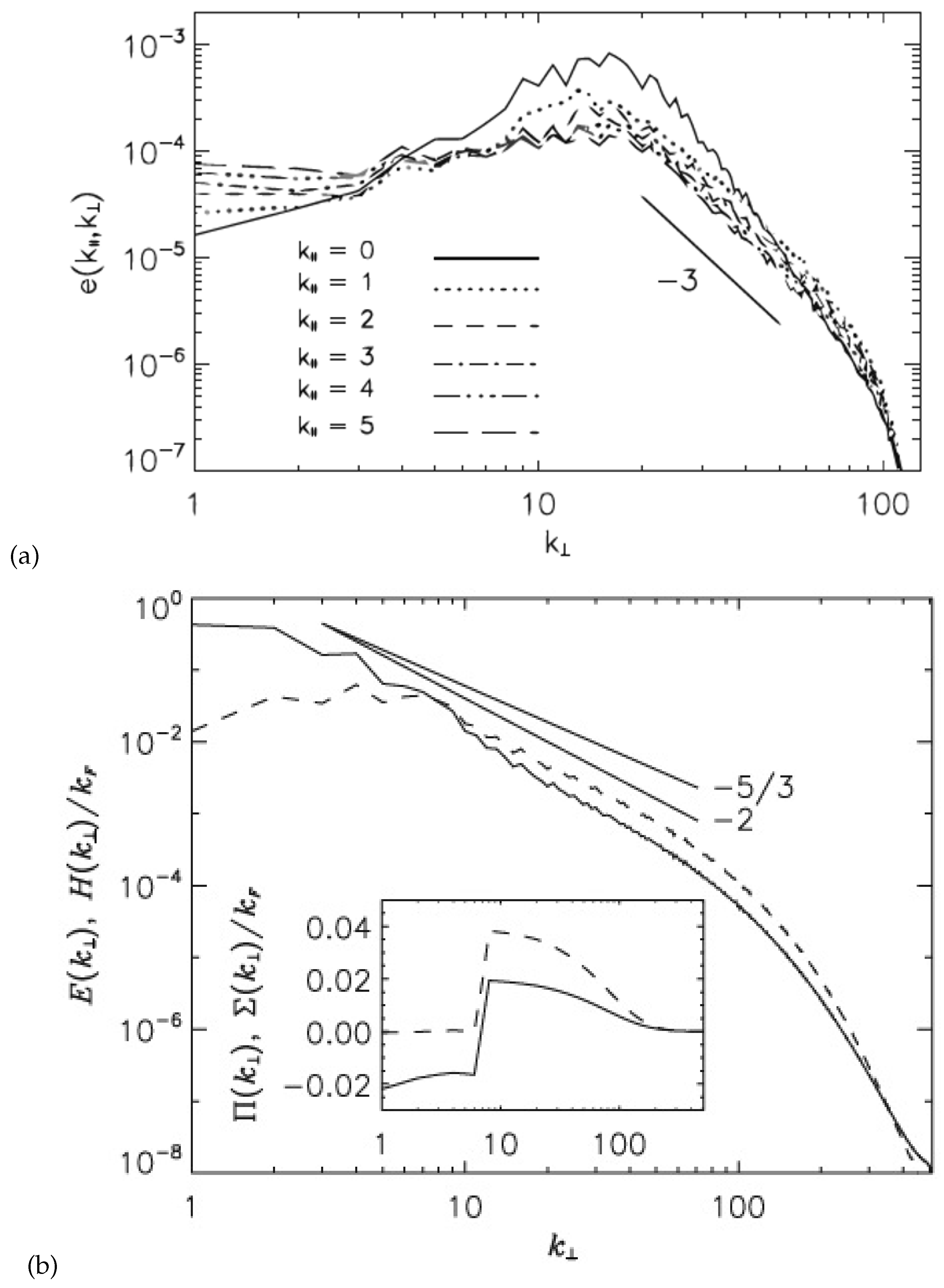
Figure 2.
Helical wave basis: forms a right-handed coordinate system with where . The wave propagation direction is given by the wave vector, (which we simply call in the body of the manuscript). Within the slow manifold where , .
Figure 2.
Helical wave basis: forms a right-handed coordinate system with where . The wave propagation direction is given by the wave vector, (which we simply call in the body of the manuscript). Within the slow manifold where , .

Figure 3.
Contour plot showing the surface of integration of the collision integral (without the constant ) in Equation (43) projected on the plane. Colors represent the value of the integrand. Figures on the left are in logarithmic scale. (a) and (b) correspond to while (c) and (d) correspond to with fixed such that . (e) is top view of (a). The singular regions are either outside the region of validity of AT (R-RHD) or correspond to identically null value of the integrand as explained in this section.

Figure 4.
Numerical integration of the collision integral in Equation (43) normalized by the constant . The plots show vs. for fixed . The integration is computed at the nodes in intervals of 20. (a) Method: Gauss Kronrod quadrature; (b) method: adaptive Monte Carlo.
Figure 4.
Numerical integration of the collision integral in Equation (43) normalized by the constant . The plots show vs. for fixed . The integration is computed at the nodes in intervals of 20. (a) Method: Gauss Kronrod quadrature; (b) method: adaptive Monte Carlo.

Figure 5.
A sketch of cascade paths for rotating turbulence shows the different flow regimes and the corresponding energy spectra. Here, is the isotropic wavenumber, is the classical critical balance wavenumber, is the injection wavenumber corresponding to an initial wave field. Three distinct regimes are shown: (i) WT (Galtier) corresponding to the wave-turbulence regime with , (ii) CB w/ pol. (i.e., critical balance with polarization alignment) as explained in [27] leading towards isotropy, and (iii) AT (R-RHD) corresponding to the anisotropic wave turbulence dynamics of the R-RHD equations with and . As we move along the horizontal axis from left to right, the flow traverses a hierarchy of slow manifolds with successively rescaled (decreasing) wave number ratio. Also shown are possible explanation of 2D-3D coupling by non-resonant interactions. The AT (R-RHD) does not explain inverse cascade phenomena as the energy flux obtained is direct. Here is the wavenumber corresponding to the initial condition.
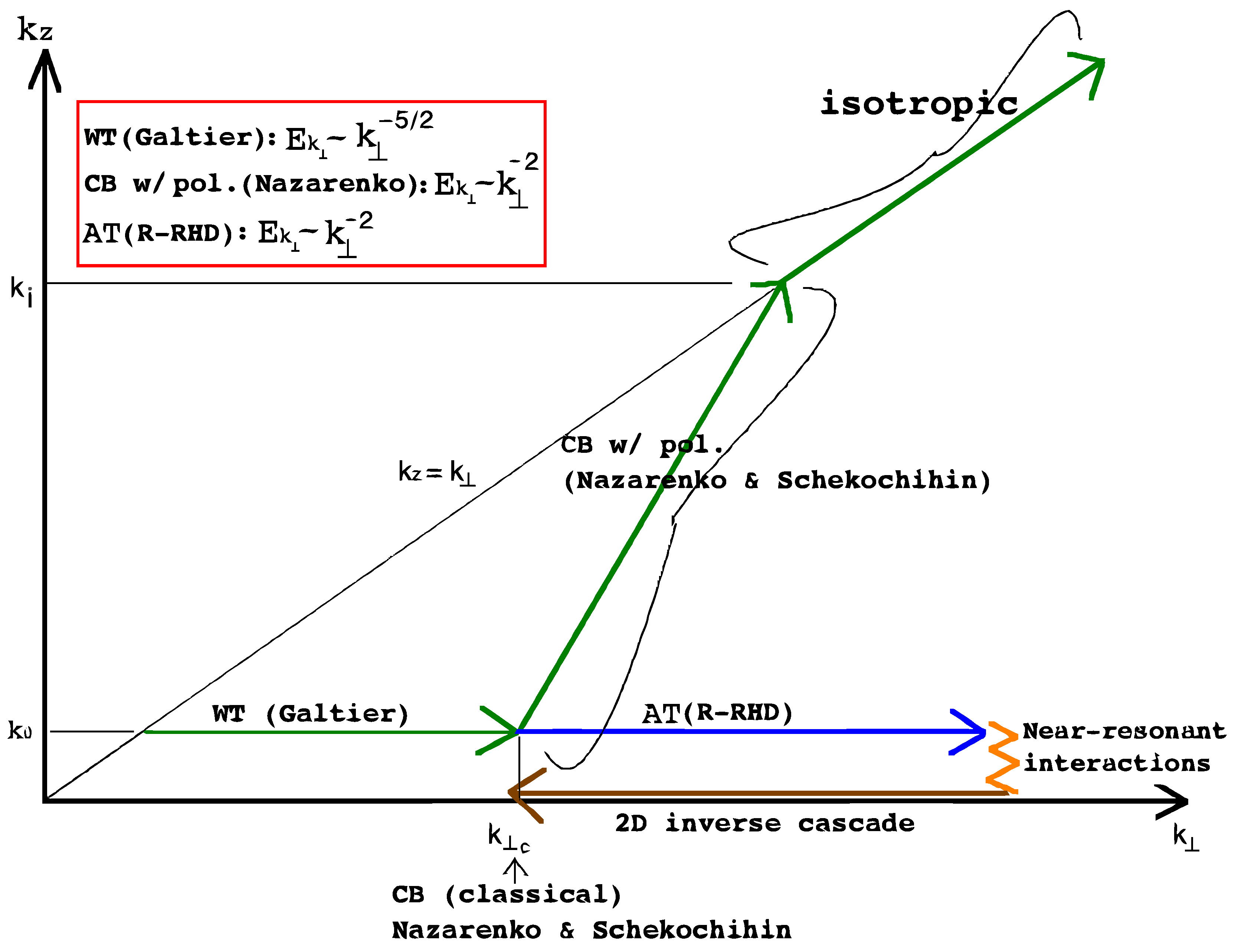
© 2017 by the author. Licensee MDPI, Basel, Switzerland. This article is an open access article distributed under the terms and conditions of the Creative Commons Attribution (CC BY) license (http://creativecommons.org/licenses/by/4.0/).
Share and Cite
MDPI and ACS Style
Sen, A. Anisotropic Wave Turbulence for Reduced Hydrodynamics with Rotationally Constrained Slow Inertial Waves. Fluids 2017, 2, 28. https://doi.org/10.3390/fluids2020028
AMA Style
Sen A. Anisotropic Wave Turbulence for Reduced Hydrodynamics with Rotationally Constrained Slow Inertial Waves. Fluids. 2017; 2(2):28. https://doi.org/10.3390/fluids2020028
Chicago/Turabian StyleSen, Amrik. 2017. "Anisotropic Wave Turbulence for Reduced Hydrodynamics with Rotationally Constrained Slow Inertial Waves" Fluids 2, no. 2: 28. https://doi.org/10.3390/fluids2020028