
Turbulence Intensity and the Friction Factor for Smooth- and Rough-Wall Pipe Flow


Toftehøj 23, Høruphav, 6470 Sydals, Denmark
Fluids 2017, 2(2), 30; https://doi.org/10.3390/fluids2020030
Submission received: 24 April 2017
/
Revised: 16 May 2017
/
Accepted: 8 June 2017
/
Published: 10 June 2017
(This article belongs to the Special Issue Turbulence: Numerical Analysis, Modelling and Simulation)
Abstract
:Turbulence intensity profiles are compared for smooth- and rough-wall pipe flow measurements made in the Princeton Superpipe. The profile development in the transition from hydraulically smooth to fully rough flow displays a propagating sequence from the pipe wall towards the pipe axis. The scaling of turbulence intensity with Reynolds number shows that the smooth- and rough-wall level deviates with increasing Reynolds number. We quantify the correspondence between turbulence intensity and the friction factor.
1. Introduction
Measurements of streamwise turbulence [1] in smooth and rough pipes have been carried out in the Princeton Superpipe [2,3,4] (Note that the author of this paper did not participate in making the Princeton Superpipe measurements.). We have treated the smooth pipe measurements as a part of [5]. In this paper, we add the rough pipe measurements to our previous analysis. The smooth (rough) pipe had a radius R of 64.68 (64.92) mm and a root mean square (RMS) roughness of 0.15 (5) m, respectively. The corresponding sand-grain roughness is 0.45 (8) m [6].
The smooth pipe is hydraulically smooth for all Reynolds numbers covered. The rough pipe evolves from hydraulically smooth through transitionally rough to fully rough with increasing . Throughout this paper, means the bulk defined using the pipe diameter D.
We define the turbulence intensity (TI) I as:
where v is the mean flow velocity, is the RMS of the turbulent velocity fluctuations and r is the radius ( is the pipe axis, is the pipe wall).
An overview of past research on turbulent flows over rough walls can be found in the pioneering work by Nikuradse [7] and a more recent review by Jiménez [8].
The development of predictive drag models has previously been carried out using both measurements [9] and direct numerical simulations (DNS) [10]. This work covered the transitionally and fully rough regimes and a variety of rough surface geometries.
The aim of this paper is to provide the fluid mechanics community with a scaling of the TI with , both for smooth- and rough-wall pipe flow. An application example is computational fluid dynamics (CFD) simulations, where the TI at an opening can be specified. A scaling expression of TI with is provided as Equation (6.62) in [11]. However, this formula does not appear to be documented, i.e., no reference is provided.
Our paper is structured as follows: in Section 2, we study how the TI profiles change over the transition from smooth to rough pipe flow. Thereafter, we present the resulting scaling of the TI with in Section 3. Quantification of the correspondence between the friction factor and the TI is contained in Section 4, and we discuss our findings in Section 5. Finally, we conclude in Section 6.
2. Turbulence Intensity Profiles
We have constructed the TI profiles for the measurements available (see Figure 1). Nine profiles are available for the smooth pipe and four for the rough pipe. In terms of , the rough pipe measurements are a subset of the smooth pipe measurements. Corresponding friction Reynolds numbers can be found in Table 1 in [3].
To make a direct comparison of the smooth and rough pipe measurements, we interpolate the smooth pipe measurements to the four values where the rough pipe measurements are done. Furthermore, we use a normalized pipe radius to account for the difference in smooth and rough pipe radii. The result is a comparison of the TI profiles at four (see Figure 2). As increases, we observe that the rough pipe TI becomes larger than the smooth pipe TI.
To make the comparison more quantitative, we define the turbulence intensity ratio (TIR):
The TIR is shown in Figure 3. The left-hand plot shows all radii; prominent features are:
- The TIR on the axis is roughly one except for the highest , where it exceeds 1.1.
- In the intermediate region between the axis and the wall, an increase is already visible for the second-lowest , 1.98 × 10⁶.
The events close to the wall are most clearly seen in the right-hand plot of Figure 3. A local peak of TIR is observed for all ; the magnitude of the peak increases with . Note that we only analyse data to 99.8% of the pipe radius. Thus, the 0.13 mm closest to the wall is not considered.
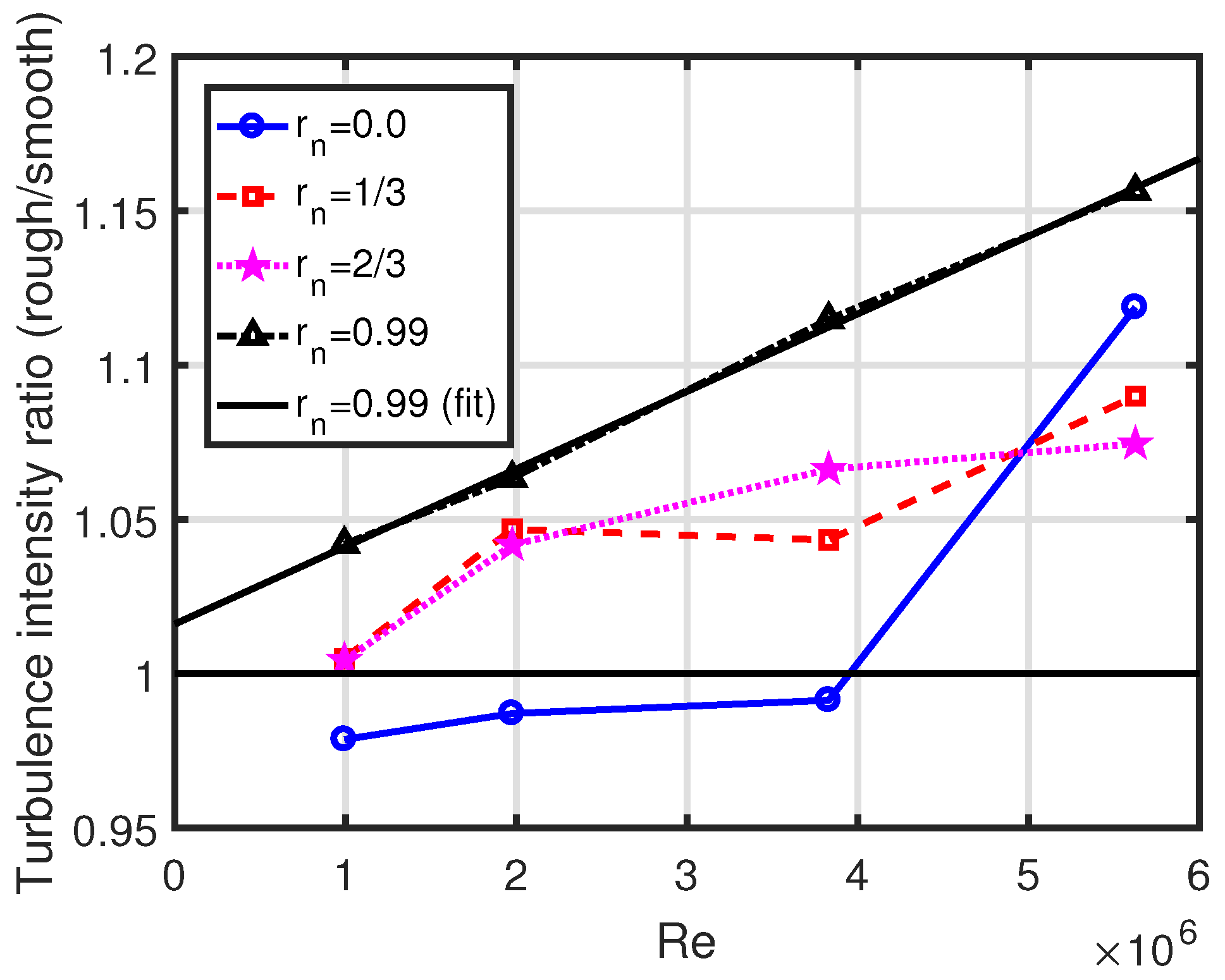
The TIR information can also be represented by studying the TIR at fixed vs. (see Figure 4). From this plot, we find that the magnitude of the peak close to the wall () increases linearly with :
Information on fits of the TI profiles to analytical expressions can be found in Appendix A.
Based on uncertainties in Table 2 in [3], the uncertainty of TI for the smooth (rough) pipe is 2.9% (3.5%), respectively. Note that we have used 4.4% instead of 4.7% for the uncertainty of to derive the rough pipe uncertainty. The resulting TIR uncertainty is 4.5%.
3. Turbulence Intensity Scaling
We define the TI averaged over the pipe area as:
In [5], another definition was used for the TI averaged over the pipe area. Analysis presented in Section 3 and Section 4 is repeated using that definition in Appendix B.
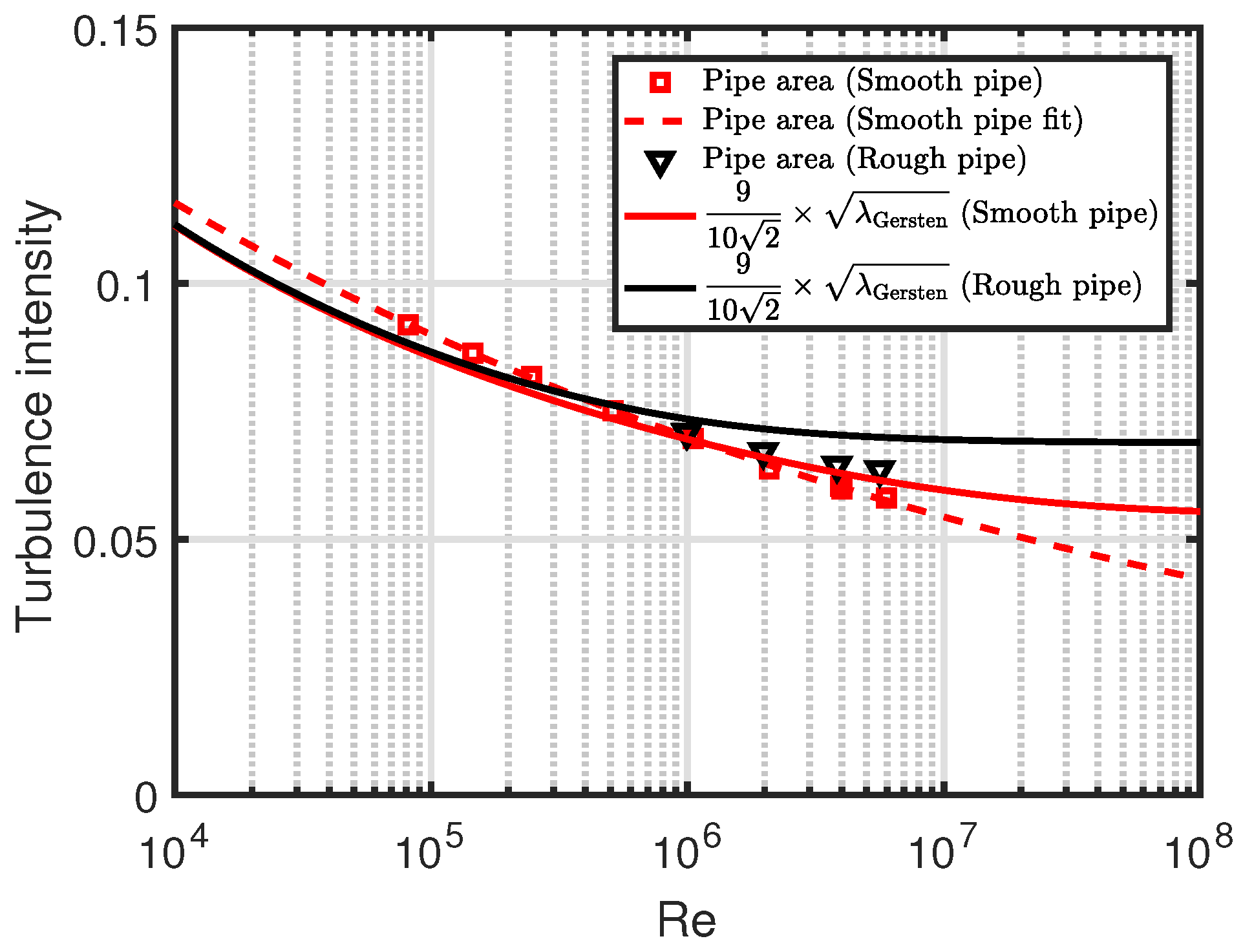
Scaling of the TI with for smooth- and rough-wall pipe flow is shown in Figure 5. For , the smooth and rough pipe values are almost the same. However, when increases, the TI of the rough pipe increases compared to the smooth pipe; this increase is to a large extent caused by the TI increase in the intermediate region between the pipe axis and the pipe wall (see Figure 3 and Figure 4). We have not made fits to the rough wall pipe measurements because of the limited number of datapoints.
4. Friction Factor
The fits shown in Figure 5 are:
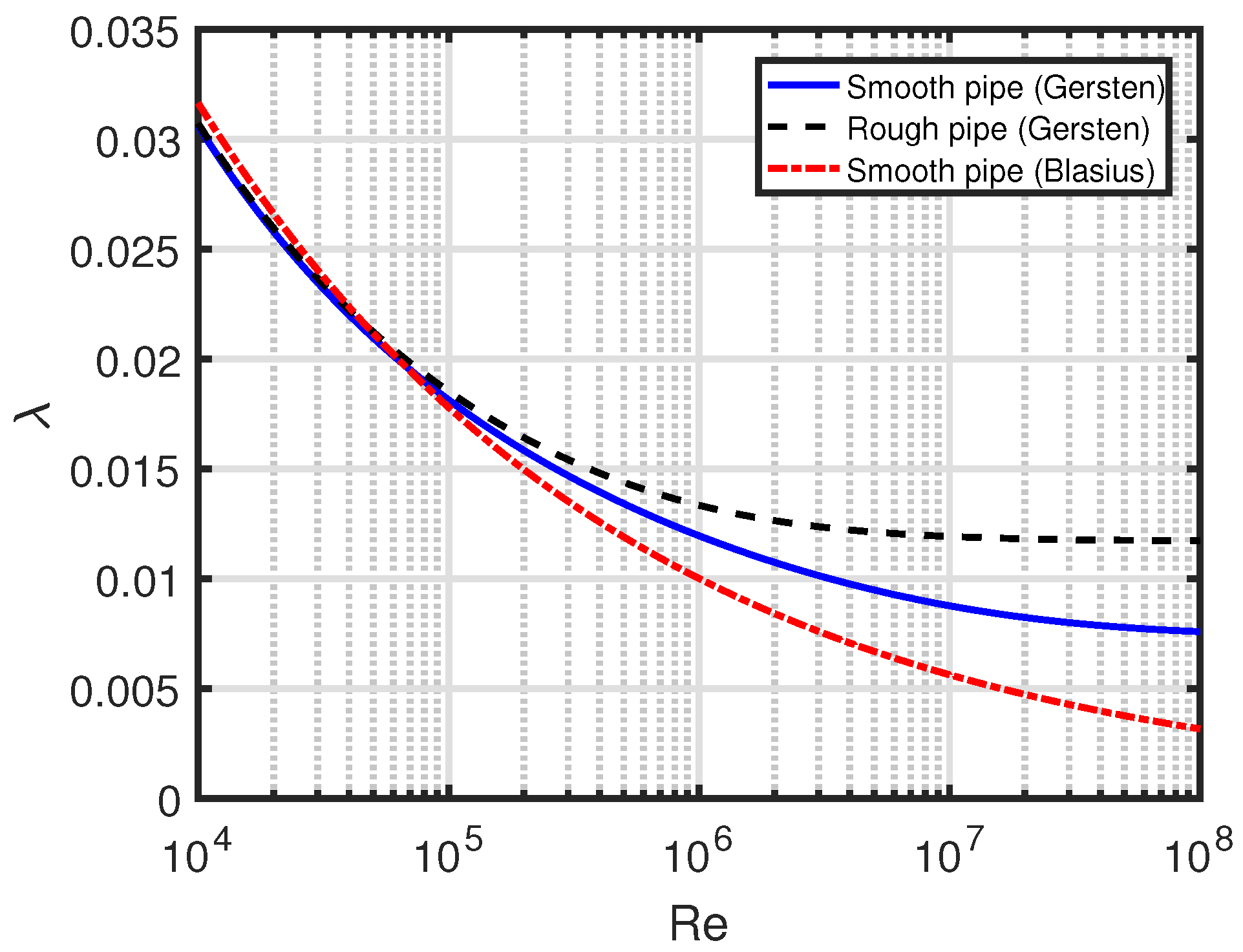
The Blasius smooth pipe (Darcy) friction factor [12] is also expressed as an power-law:
The Blasius friction factor matches measurements best for ; the friction factor by e.g., Gersten (Equation (1.77) in [13]) is preferable for larger . The Blasius and Gersten friction factors are compared in Figure 6. The deviation between the smooth and rough pipe Gersten friction factors above is qualitatively similar to the deviation between the smooth and rough pipe area TI in Figure 5. For the Gersten friction factors, we have used the measured pipe roughnesses.
For the smooth pipe, we can combine Equations (5) and (6) to relate the pipe area TI to the Blasius friction factor:
The TI and Blasius friction factor scaling is shown in Figure 7.
For axisymmetric flow in the streamwise direction, the mean flow velocity averaged over the pipe area is:
Now, we are in a position to define an average velocity of the turbulent fluctuations:
The friction velocity is:
where is the wall shear stress and is the fluid density.
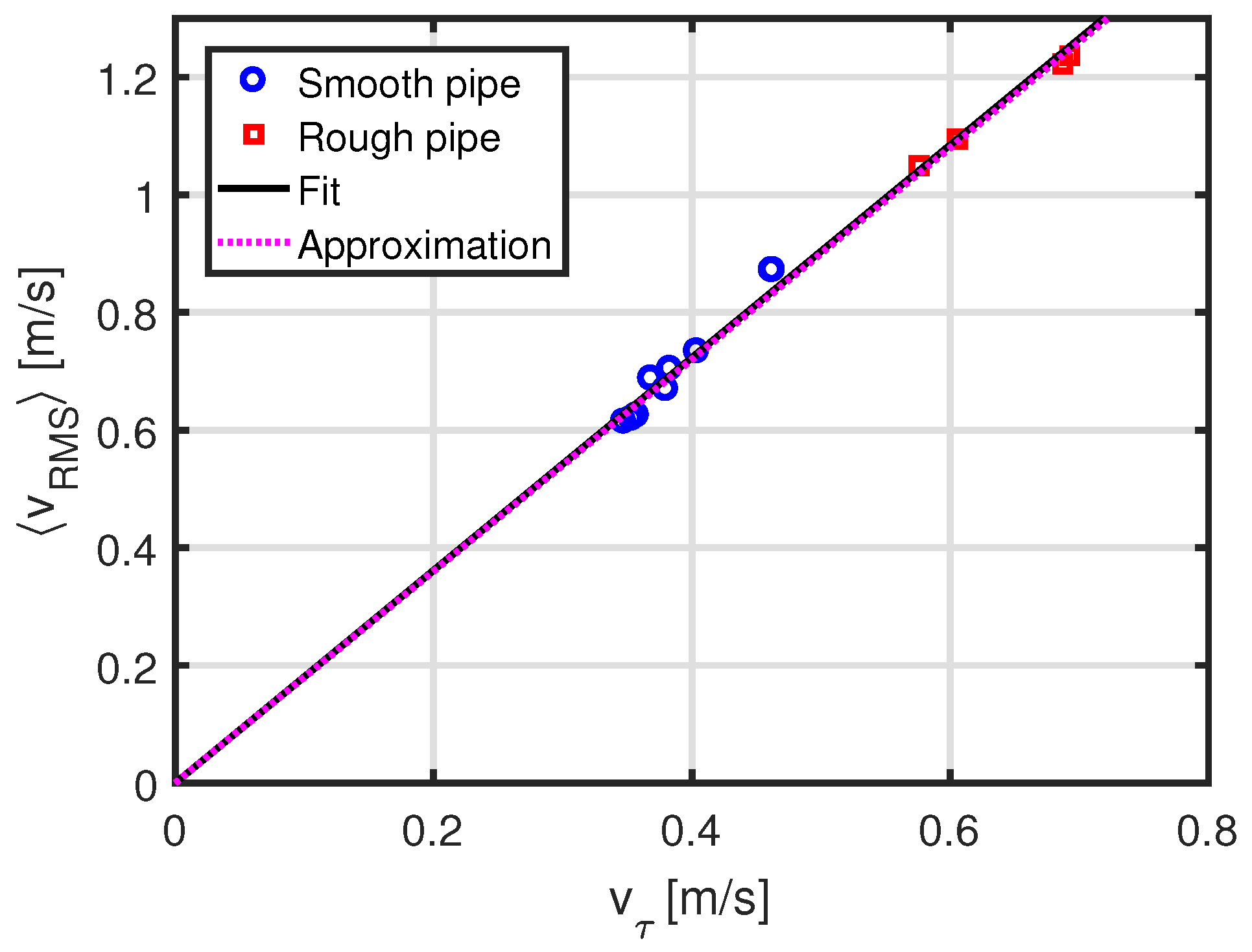
The relationship between and is illustrated in Figure 8. From the fit, we have:
which we approximate as:
Equations (11) and (12) above correspond to the usage of the friction velocity as a proxy for the velocity of the turbulent fluctuations [14]. We note that the rough wall velocities are higher than for the smooth wall.
Equations (9) and (12) can be combined with Equation (1.1) in [15]:
where is the pressure loss and L is the pipe length. This can be reformulated as:
We show how well this approximation works in Figure 9. Overall, the agreement is within 15%.
We proceed to define the average kinetic energy of the turbulent velocity fluctuations (per pipe volume V) as:
with , so we have:
where m is the fluid mass. The pressure loss corresponds to an increase of the turbulent kinetic energy. The turbulent kinetic energy can also be expressed in terms of the mean flow velocity and the TI or the friction factor:
5. Discussion
5.1. The Attached Eddy Hypothesis
Our quantification of the ratio as a constant can be placed in the context of the attached eddy hypothesis by Townsend [16,17]. Our results are for quantities averaged over the pipe radius, whereas the attached eddy hypothesis provides a local scaling with distance from the wall. By proposing an overlap region (see Figure 1 in [18]) between the inner and outer scaling [19], it can be deduced that is a constant in this overlap region [20,21]. Such an overlap region has been shown to exist in [2,20]. The attached eddy hypothesis has provided the basis for theoretical work on e.g., the streamwise turbulent velocity fluctuations in flat-plate [22] and pipe flow [23] boundary layers. Work on the law of the wake in wall turbulence also makes use of the attached eddy hypothesis [24].
As a consistency check for our results, we can compare the constant in Equation (12) to the prediction by Townsend:
where fits have provided the constants and . Here, is a universal constant, whereas is not expected to be a constant for different wall-bounded flows [25]. The constants are averages of fits presented in [3] to the smooth- and rough-wall Princeton Superpipe measurements. The Townsend-Perry constant was found to be 1.26 in [25]. Performing the area averaging yields:
5.2. The Friction Factor and Turbulent Velocity Fluctuations
The proportionality between the average kinetic energy of the turbulent velocity fluctuations and the friction velocity squared has been identified in [27] for . This corresponds to our Equation (16).
A correspondence between the wall-normal Reynolds stress and the friction factor has been shown in [28]. Those results were found using DNS. The main difference between the cases is that we use the streamwise Reynolds stress. However, for an eddy rotating in the streamwise direction, both a wall-normal and a streamwise component should exist which connects the two observations.
5.3. The Turbulence Intensity and the Diagnostic Plot
Other related work can be found beginning with [29] where the diagnostic plot was introduced. In the following publications, a version of the diagnostic plot was brought forward where the local TI is plotted as a function of the local streamwise velocity normalised by the free stream velocity [30,31,32]. Equation (3) in [31] corresponds to our (see Equation (A1) in Appendix A).
5.4. Applicability of Turbulence Intensity Scaling with Friction Factor
The scaling of TI with the friction factor (Equation (14)) was found based on pipe flow measurements with two roughnesses. It is an open question whether our result holds in the fully rough regime. For the fully rough regime, the friction factor becomes a constant for high . As a consequence of our scaling expression, this should also be the case for the TI.
It is clear that the specific formula is not directly applicable for other wall-bounded flows, since takes different values. However, the basic behaviour, i.e., that the TI scales with the square root of the friction factor, may be universally valid.
6. Conclusions
We have compared TI profiles for smooth- and rough-wall pipe flow measurements made in the Princeton Superpipe.
The change of the TI profile with increasing from hydraulically smooth to fully rough flow exhibits propagation from the pipe wall to the pipe axis. The TIR at scales linearly with .
The scaling of TI with —on the pipe axis and averaged over the pipe area—shows that the smooth- and rough-wall level deviates with increasing Reynolds number.
We find that . This relationship can be useful to calculate the TI given a known , both for smooth and rough pipes. It follows that given a pressure loss in a pipe, the turbulent kinetic energy increase can be estimated.
Acknowledgments
We thank Alexander J. Smits for making the Superpipe data publicly available.
Conflicts of Interest
The authors declare no conflict of interest.
Appendix A. Fits to the Turbulence Intensity Profile
As we have done for the smooth pipe measurements in [5], we can also fit the rough pipe measurements to this function:
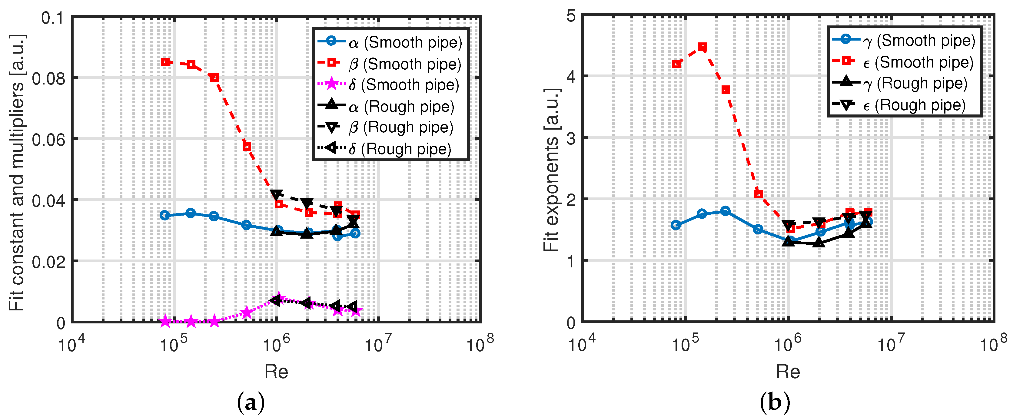
where , , , and are fit parameters. A comparison of fit parameters found for the smooth- and rough-pipe measurements is shown in Figure A1. Overall, we can state that the fit parameters for the smooth and rough pipes are in a similar range for .
Figure A1.
Comparison of smooth- and rough-pipe fit parameters, (a): fit parameters , and ; (b): fit parameters and .
Figure A1.
Comparison of smooth- and rough-pipe fit parameters, (a): fit parameters , and ; (b): fit parameters and .

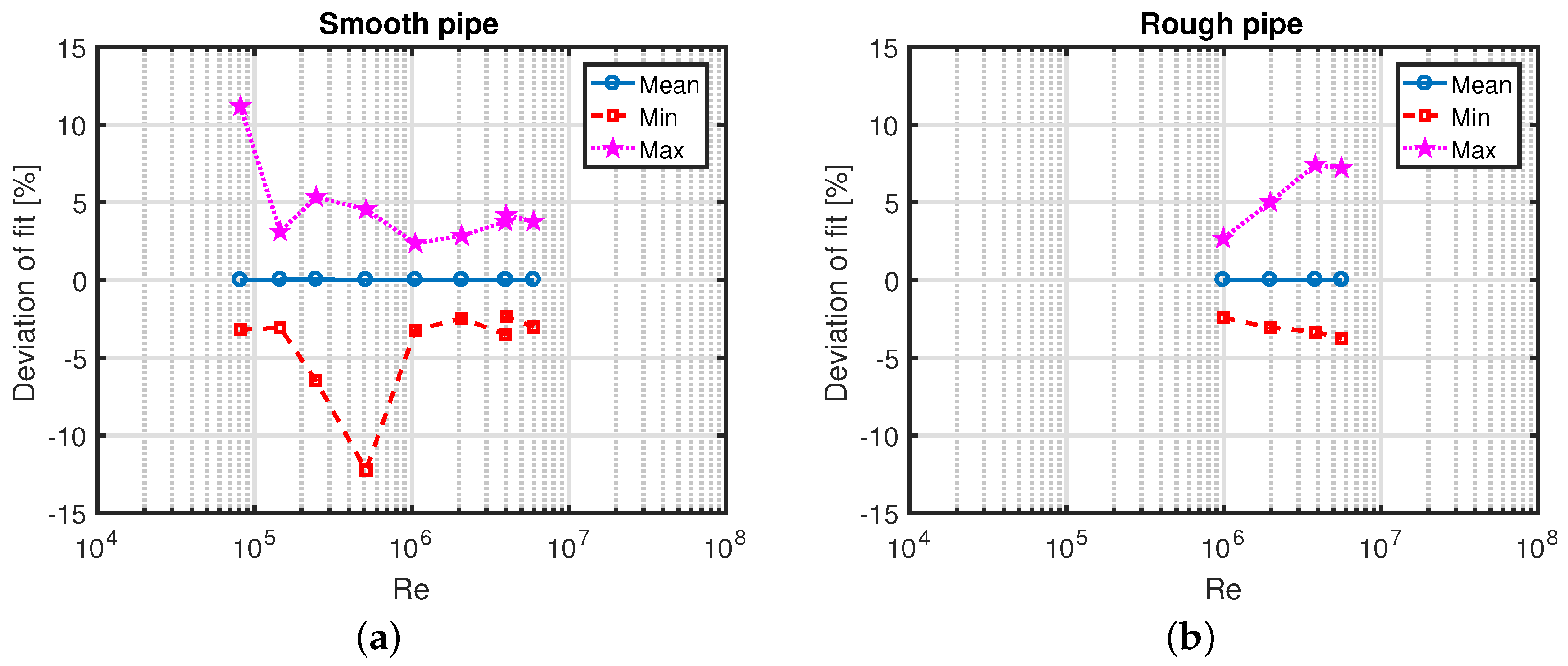
The min/max deviation of the rough pipe fit from the measurements is below 10%; see the comparison to the smooth wall fit min/max deviation in Figure A2.
Figure A2.
Deviation of fits to measurements; (a): smooth pipe, (b): rough pipe.
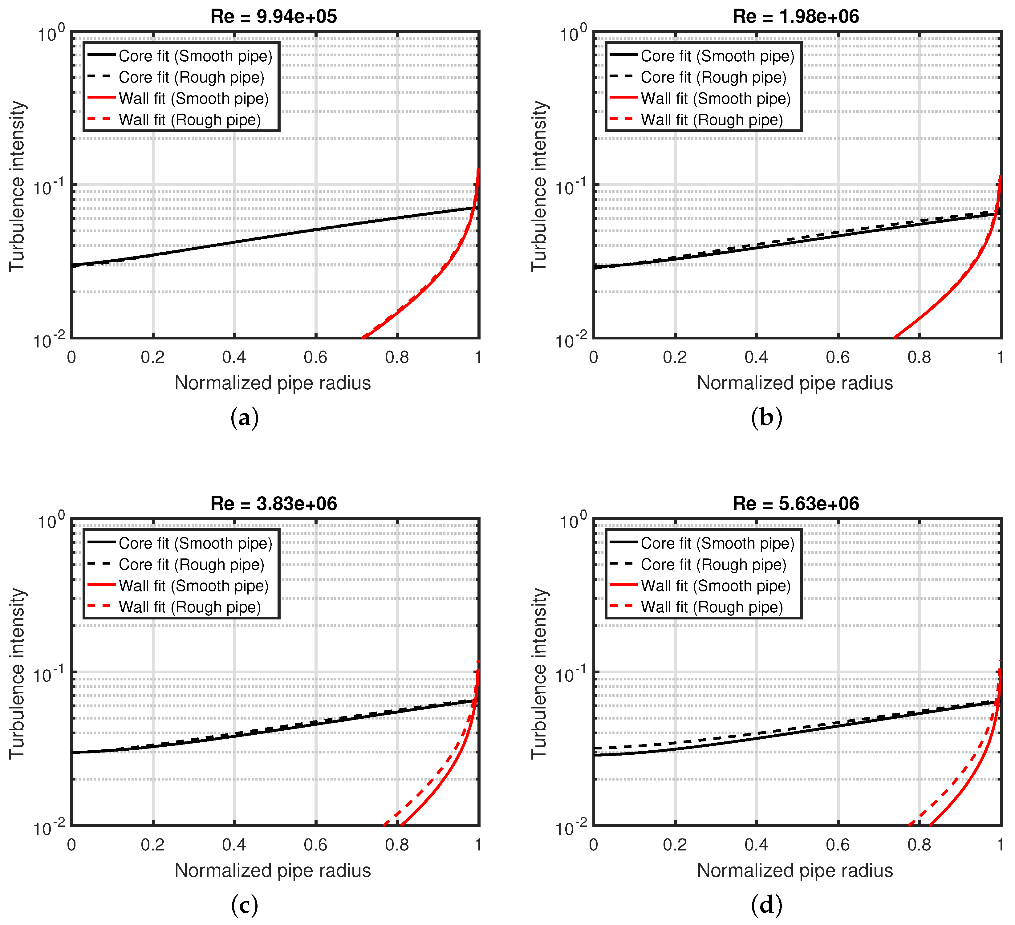
The core and wall fits for the smooth and rough pipe fits are compared in Figure A3.
Figure A3.
Comparison of smooth and rough pipe core and wall fits, (a): Re = 9.94e + 05; (b): Re = 1.98e + 06; (c): Re = 3.83e + 06; (d): Re = 5.63e + 06.
Figure A3.
Comparison of smooth and rough pipe core and wall fits, (a): Re = 9.94e + 05; (b): Re = 1.98e + 06; (c): Re = 3.83e + 06; (d): Re = 5.63e + 06.
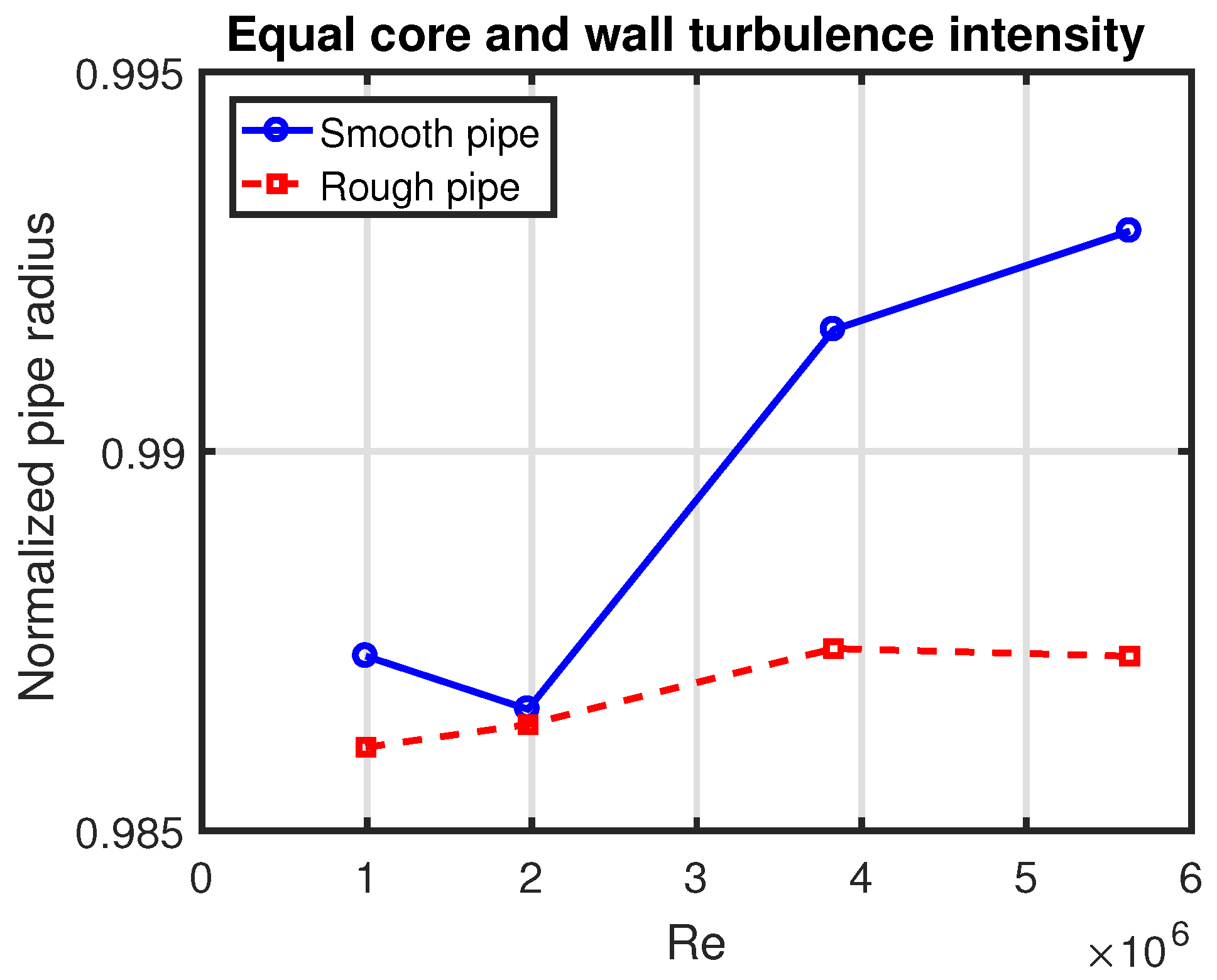
The position where the core and wall TI levels are equal is shown in Figure A4. This position does not change significantly for the rough pipe; however, the position does increase with for the smooth pipe: this indicates that the wall term becomes less important relative to the core term.
Figure A4.
Normalised pipe radius where the core and wall TI levels are equal.
Appendix B. Arithmetic Mean Definition of Turbulence Intensity Averaged Over the Pipe Area
In the main paper, we have defined the TI over the pipe area in Equation (4). In [5], we used the arithmetic mean (AM) instead:
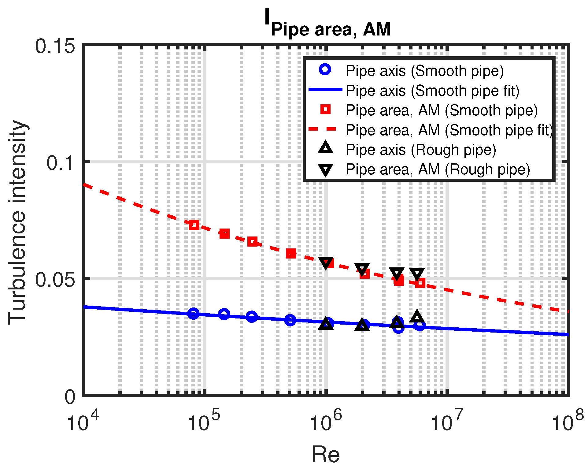
The AM leads to a somewhat different pipe area scaling for the smooth pipe measurements, which is illustrated in Figure A5. Compare to Figure 5.
Figure A5.
Turbulence intensity for smooth and rough pipe flow. The arithmetic mean (AM) is used for the pipe area TI.
Figure A5.
Turbulence intensity for smooth and rough pipe flow. The arithmetic mean (AM) is used for the pipe area TI.

The scaling found in [5] using this definition is:
The AM scaling also has implications for the relationship with the Blasius friction factor scaling (Equation (7)):
We can now define the AM version of the average velocity of the turbulent fluctuations:
The AM definition can be considered as a first order moment equation for , whereas the definition in Equation (9) is a second order moment equation.
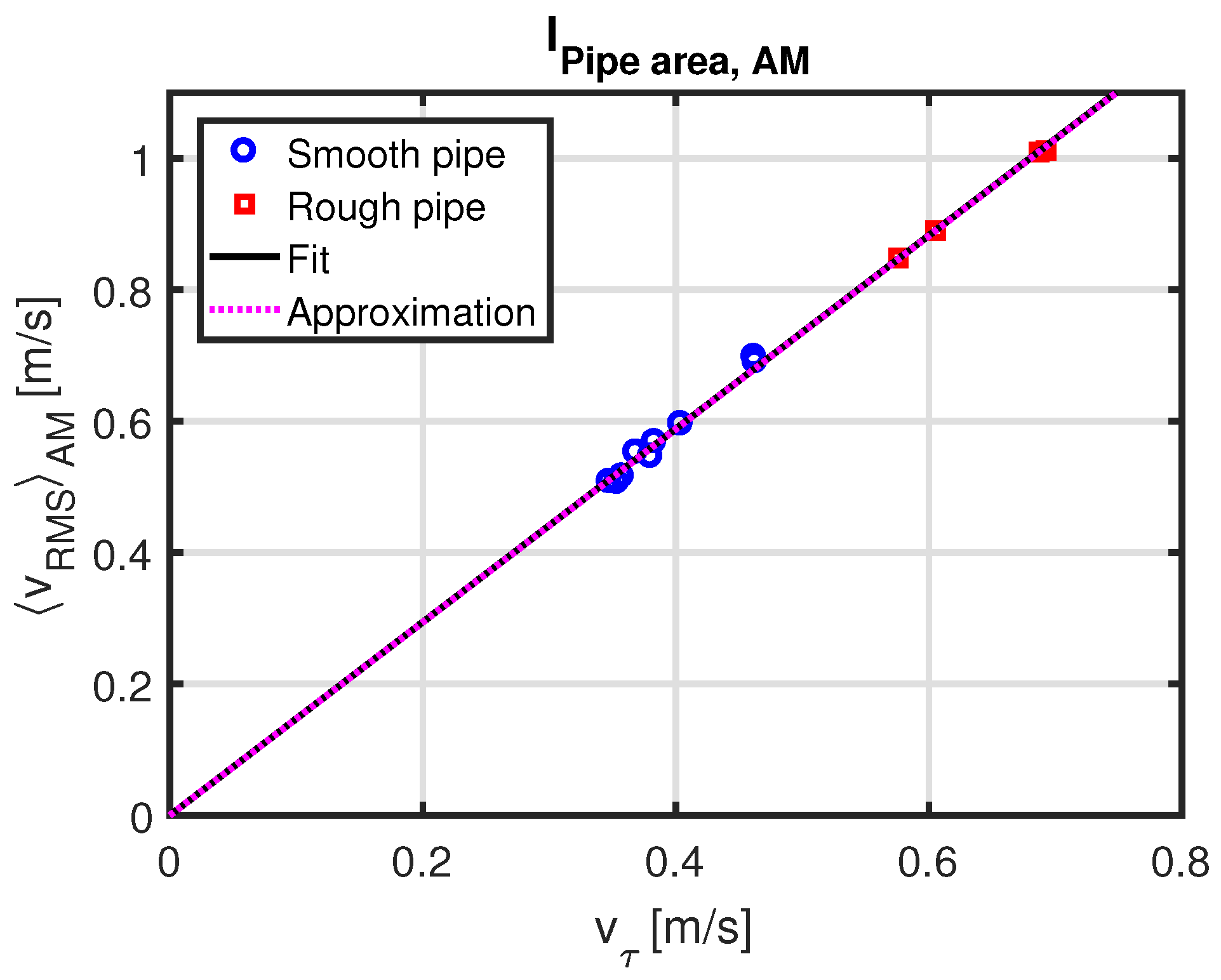
Again, we find that the AM average turbulent velocity fluctuations are proportional to the friction velocity. However, the constant of proportionality is different than the one in Equation (11) (see Figure A6). The AM case can be fitted as:
which we approximate as:
Figure A6.
Relationship between friction velocity and the AM average velocity of the turbulent fluctuations.
Figure A6.
Relationship between friction velocity and the AM average velocity of the turbulent fluctuations.
References
- Marusic, I.; McKeon, B.J.; Monkewitz, P.A.; Nagib, H.M.; Smits, A.J.; Sreenivasan, K.R. Wall-bounded turbulent flows at high Reynolds numbers: Recent advances and key issues. Phys. Fluids 2010, 22, 065103. [Google Scholar] [CrossRef]
- Hultmark, M.; Vallikivi, M.; Bailey, S.C.C.; Smits, A.J. Turbulent pipe flow at extreme Reynolds numbers. Phys. Rev. Lett. 2012, 108, 094501. [Google Scholar] [CrossRef] [PubMed]
- Hultmark, M.; Vallikivi, M.; Bailey, S.C.C.; Smits, A.J. Logarithmic scaling of turbulence in smooth- and rough-wall pipe flow. J. Fluid Mech. 2013, 728, 376–395. [Google Scholar] [CrossRef]
- Princeton Superpipe. 2017. Available online: https://smits.princeton.edu/superpipe-turbulence-data/ (accessed on 7 June 2017).
- Russo, F.; Basse, N.T. Scaling of turbulence intensity for low-speed flow in smooth pipes. Flow Meas. Instrum. 2016, 52, 101–114. [Google Scholar] [CrossRef]
- Langelandsvik, L.I.; Kunkel, G.J.; Smits, A.J. Flow in a commercial steel pipe. J. Fluid Mech. 2008, 595, 323–339. [Google Scholar] [CrossRef]
- Nikuradse, J. Strömungsgesetze in Rauhen Rohren; Springer-VDI-Verlag GmbH: Düsseldorf, Germany, 1933. [Google Scholar]
- Jiménez, J. Turbulent flows over rough walls. Annu. Rev. Fluid Mech. 2004, 36, 173–196. [Google Scholar] [CrossRef]
- Flack, K.A.; Schultz, M.P. Review of hydraulic roughness scales in the fully rough regime. J. Fluids Eng. 2010, 132, 041203. [Google Scholar] [CrossRef]
- Chan, L.; MacDonald, M.; Chung, D.; Hutchins, N.; Ooi, A. A systematic investigation of roughness height and wavelength in turbulent pipe flow in the transitionally rough regime. J. Fluid Mech. 2015, 771, 743–777. [Google Scholar] [CrossRef]
- ANSYS Fluent User’s Guide, Release 18.0. 2017. Available online: http://www.ansys.com/products/fluids/ (accessed on 7 June 2017).
- Blasius, H. Das Ähnlichkeitsgesetz bei Reibungsvorgängen in Flüssigkeiten; Springer-VDI-Verlag GmbH: Düsseldorf, Germany, 1913; pp. 1–40. [Google Scholar]
- Gersten, K. Fully developed turbulent pipe flow. In Fluid Mechanics of Flow Metering; Merzkirch, W., Ed.; Springer: Berlin, Germany, 2005. [Google Scholar]
- Schlichting, H.; Gersten, K. Boundary-Layer Theory, 8th ed.; Springer: Berlin, Germany, 2000. [Google Scholar]
- McKeon, B.J.; Zagarola, M.V.; Smits, A.J. A new friction factor relationship for fully developed pipe flow. J. Fluid Mech. 2005, 538, 429–443. [Google Scholar] [CrossRef]
- Townsend, A.A. The Structure of Turbulent Shear Flow, 2nd ed.; Cambridge University Press: Cambridge, UK, 1976. [Google Scholar]
- Marusic, I.; Nickels, T.N.A.A. Townsend. In A Voyage through Turbulence; Davidson, P.A., Kaneda, Y., Moffatt, K., Sreenivasan, K.R., Eds.; Cambridge University Press: Cambridge, UK, 2011. [Google Scholar]
- McKeon, B.J.; Morrison, J.F. Asymptotic scaling in turbulent pipe flow. Phil. Trans. Royal Soc. A 2007, 365, 771–787. [Google Scholar] [CrossRef] [PubMed]
- Millikan, C.B. A critical discussion of turbulent flows in channels and circular tubes. In Proceedings of the 5th International Congress for Applied Mechanics, New York, NY, USA, 12–16 September 1938. [Google Scholar]
- Perry, A.E.; Abell, C.J. Scaling laws for pipe-flow turbulence. J. Fluid Mech. 1975, 67, 257–271. [Google Scholar] [CrossRef]
- Perry, A.E.; Abell, C.J. Asymptotic similarity of turbulence structures in smooth- and rough-walled pipes. J. Fluid Mech. 1977, 79, 785–799. [Google Scholar] [CrossRef]
- Marusic, I.; Kunkel, G.J. Streamwise turbulence intensity formulation for flat-plate boundary layers. Phys. Fluids 2003, 15, 2461–2464. [Google Scholar] [CrossRef]
- Hultmark, M. A theory for the streamwise turbulent fluctuations in high Reynolds number pipe flow. J. Fluid Mech. 2012, 707, 575–584. [Google Scholar] [CrossRef]
- Krug, D.; Philip, K.; Marusic, I. Revisiting the law of the wake in wall turbulence. J. Fluid Mech. 2017, 811, 421–435. [Google Scholar] [CrossRef]
- Marusic, I.; Monty, J.P.; Hultmark, M.; Smits, A.J. On the logarithmic region in wall turbulence. JFM Rapids 2013, 716, R3. [Google Scholar] [CrossRef]
- Pullin, D.I.; Inoue, M.; Saito, N. On the asymptotic state of high Reynolds number, smooth-wall turbulent flows. Phys. Fluids 2013, 25, 015116. [Google Scholar] [CrossRef]
- Yakhot, V.; Bailey, S.C.C.; Smits, A.J. Scaling of global properties of turbulence and skin friction in pipe and channel flows. J. Fluid Mech. 2010, 652, 65–73. [Google Scholar] [CrossRef]
- Orlandi, P. The importance of wall-normal Reynolds stress in turbulent rough channel flows. Phys. Fluids 2013, 25, 110813. [Google Scholar] [CrossRef]
- Alfredsson, P.H.; Örlü, R. The diagnostic plot—A litmus test for wall bounded turbulence data. Eur. J. Mech. B Fluids 2010, 29, 403–406. [Google Scholar] [CrossRef]
- Alfredsson, P.H.; Segalini, A.; Örlü, R. A new scaling for the streamwise turbulence intensity in wall-bounded turbulent flows and what it tells us about the “outer” peak. Phys. Fluids 2011, 23, 041702. [Google Scholar] [CrossRef]
- Alfredsson, P.H.; Örlü, R.; Segalini, A. A new formulation for the streamwise turbulence intensity distribution in wall-bounded turbulent flows. Eur. J. Mech. B Fluids 2012, 36, 167–175. [Google Scholar] [CrossRef]
- Castro, I.P.; Segalini, A.; Alfredsson, P.H. Outer-layer turbulence intensities in smooth- and rough-wall boundary layers. J. Fluid Mech. 2013, 727, 119–131. [Google Scholar] [CrossRef]
Figure 1.
Turbulence intensity as a function of pipe radius, (a): smooth pipe; (b): rough pipe.
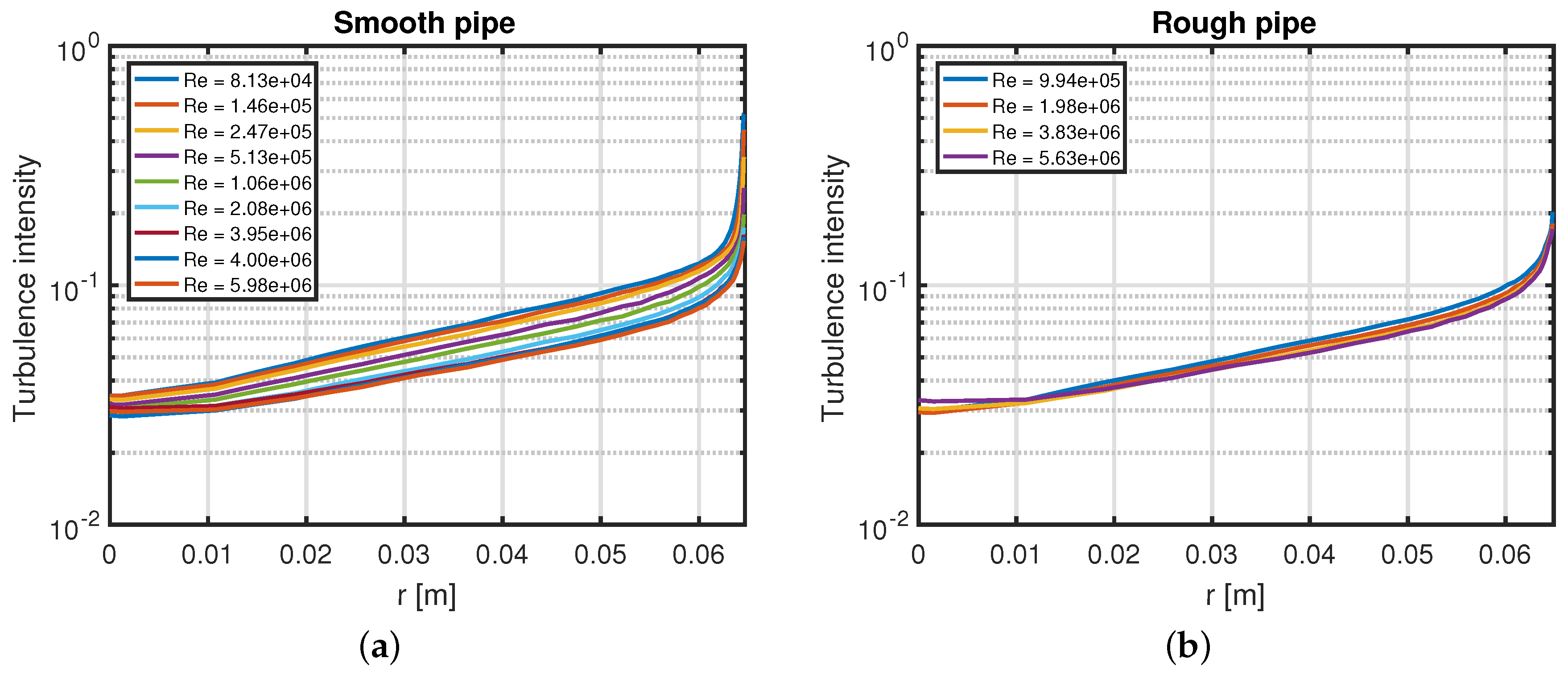
Figure 2.
Comparison of smooth and rough pipe turbulence intensity (TI) profiles for the four values where the rough pipe measurements are done, (a): Re = 9.94e + 05; (b): Re = 1.98e + 06; (c): Re = 3.83e + 06; (d): Re = 5.63e + 06.
Figure 2.
Comparison of smooth and rough pipe turbulence intensity (TI) profiles for the four values where the rough pipe measurements are done, (a): Re = 9.94e + 05; (b): Re = 1.98e + 06; (c): Re = 3.83e + 06; (d): Re = 5.63e + 06.
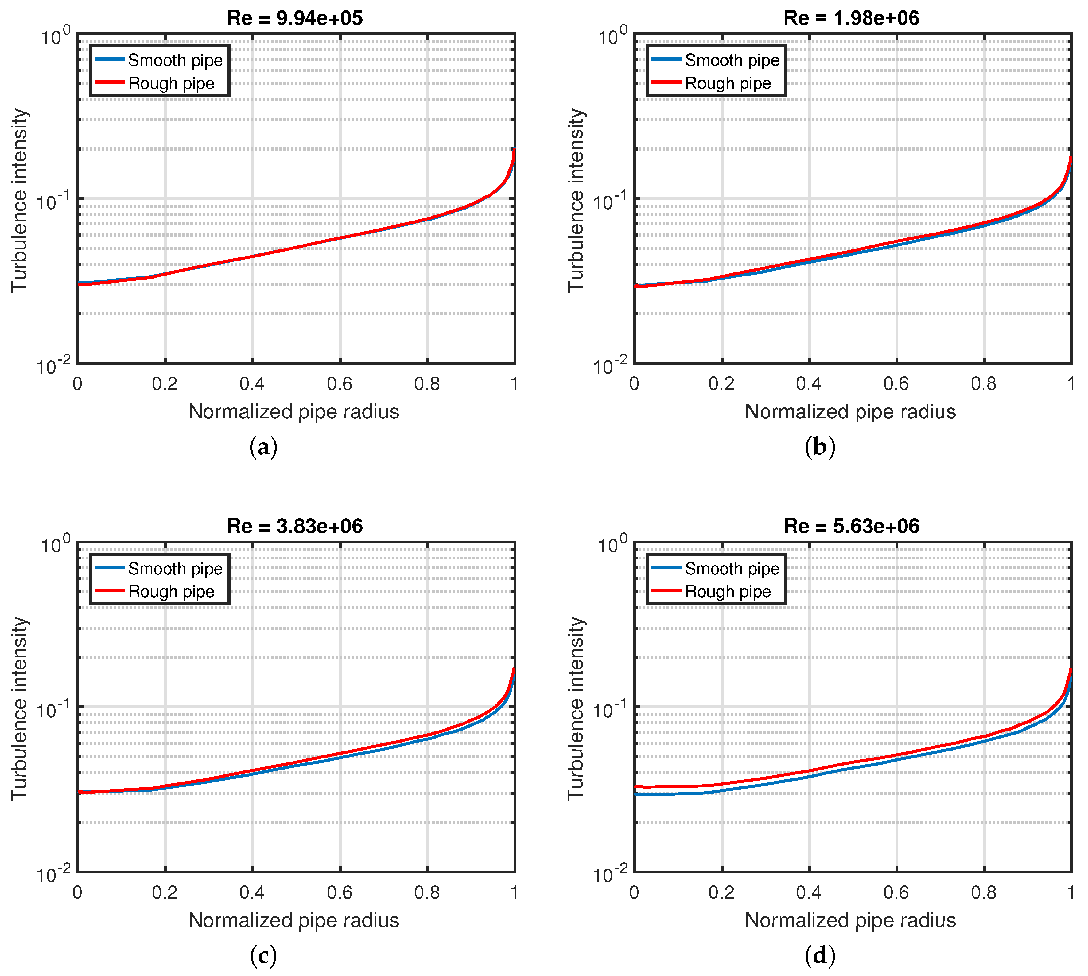
Figure 3.
Turbulence intensity ratio (TIR); (a): all radii; (b): zoom to outer 5%.
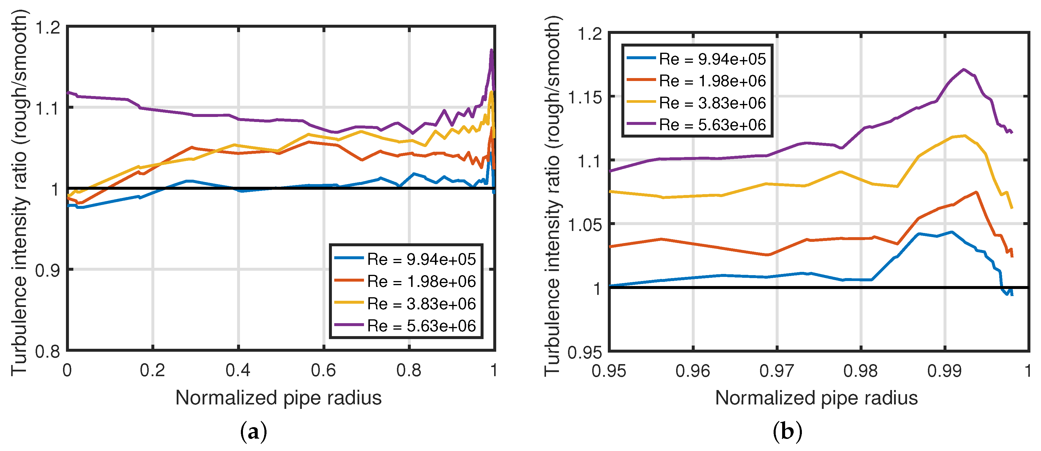
Figure 4.
Turbulence intensity ratios for fixed .

Figure 5.
Turbulence intensity for smooth and rough pipe flow.
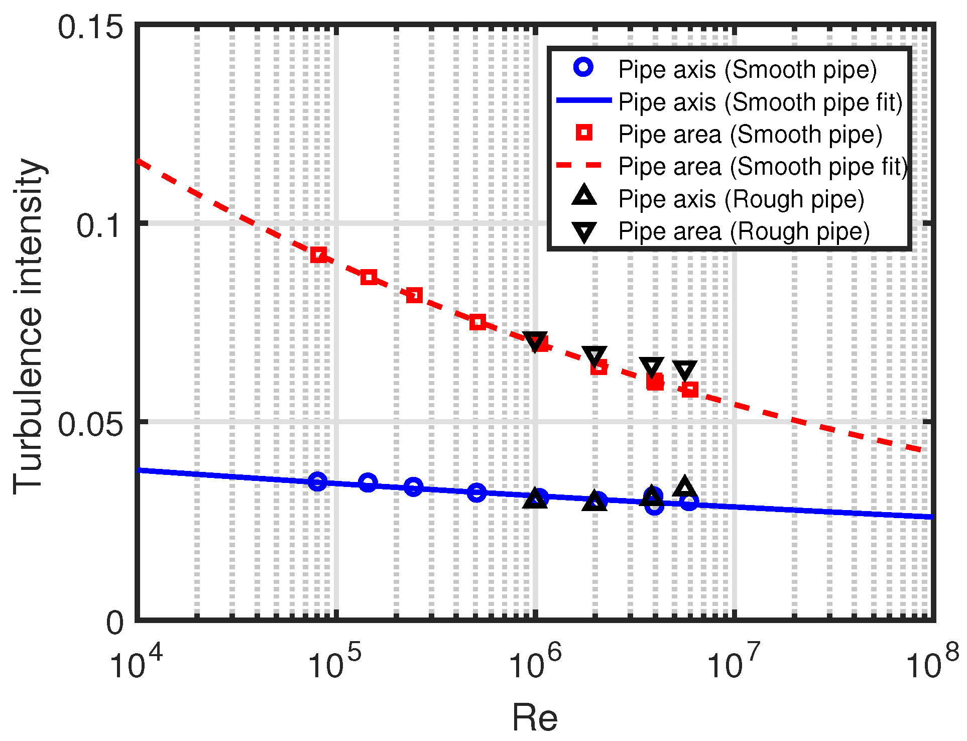
Figure 6.
Friction factor.

Figure 7.
Relationship between pipe area turbulence intensity and the Blasius friction factor.
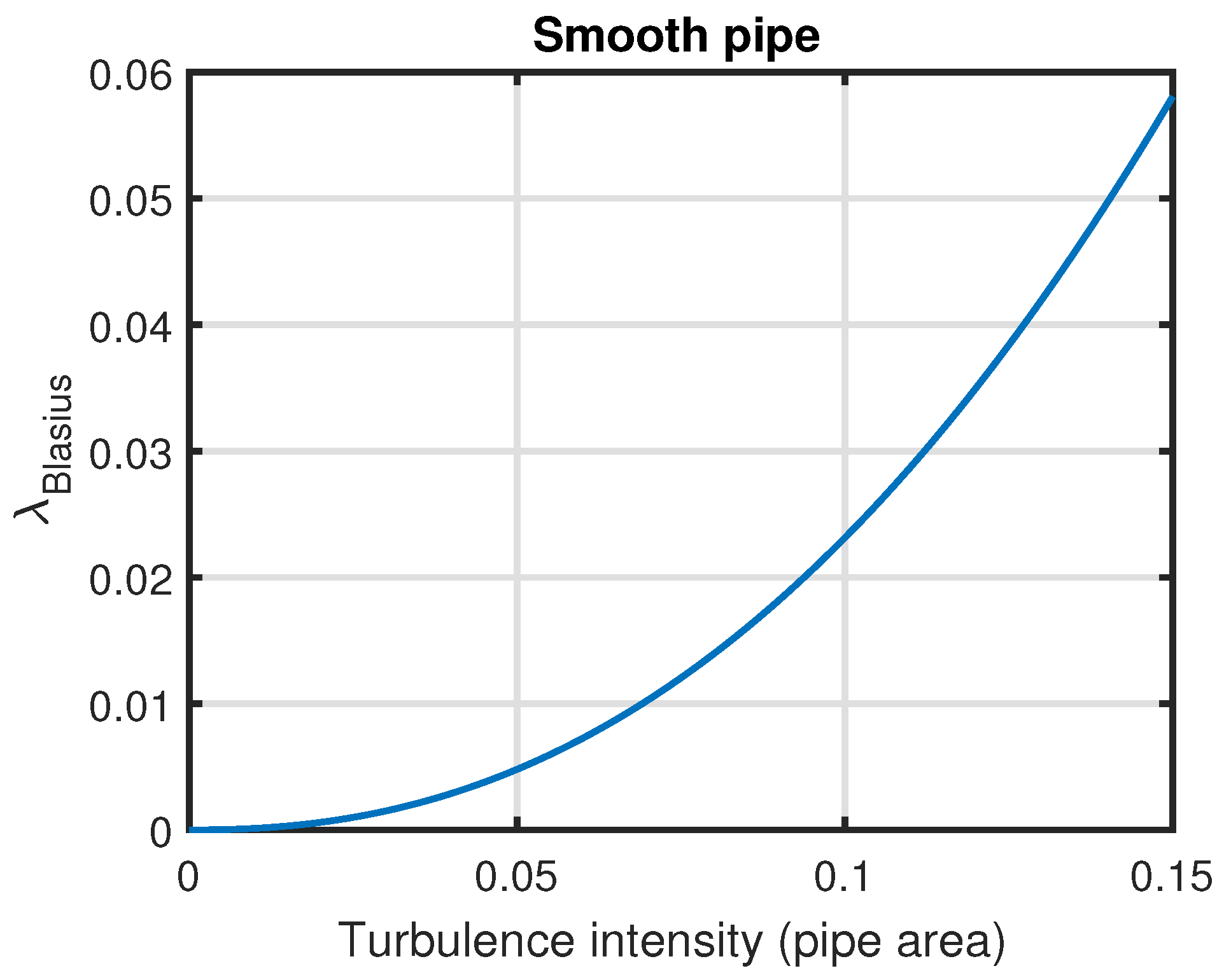
Figure 8.
Relationship between friction velocity and the average velocity of the turbulent fluctuations.
Figure 8.
Relationship between friction velocity and the average velocity of the turbulent fluctuations.

Figure 9.
Turbulence intensity for smooth and rough pipe flow. The approximation in Equation (14) is included for comparison.
Figure 9.
Turbulence intensity for smooth and rough pipe flow. The approximation in Equation (14) is included for comparison.

© 2017 by the author. Licensee MDPI, Basel, Switzerland. This article is an open access article distributed under the terms and conditions of the Creative Commons Attribution (CC BY) license (http://creativecommons.org/licenses/by/4.0/).
Share and Cite
MDPI and ACS Style
Basse, N.T. Turbulence Intensity and the Friction Factor for Smooth- and Rough-Wall Pipe Flow. Fluids 2017, 2, 30. https://doi.org/10.3390/fluids2020030
AMA Style
Basse NT. Turbulence Intensity and the Friction Factor for Smooth- and Rough-Wall Pipe Flow. Fluids. 2017; 2(2):30. https://doi.org/10.3390/fluids2020030
Chicago/Turabian StyleBasse, Nils T. 2017. "Turbulence Intensity and the Friction Factor for Smooth- and Rough-Wall Pipe Flow" Fluids 2, no. 2: 30. https://doi.org/10.3390/fluids2020030