
Convective to Absolute Instability Transition in a Horizontal Porous Channel with Open Upper Boundary


Department of Industrial Engineering, Alma Mater Studiorum Università di Bologna, Viale Risorgimento 2, 40136 Bologna, Italy
*
Author to whom correspondence should be addressed.
Fluids 2017, 2(2), 33; https://doi.org/10.3390/fluids2020033
Submission received: 28 April 2017
/
Revised: 9 June 2017
/
Accepted: 10 June 2017
/
Published: 14 June 2017
(This article belongs to the Special Issue Convective Instability in Porous Media)
Abstract
:A linear stability analysis of the parallel uniform flow in a horizontal channel with open upper boundary is carried out. The lower boundary is considered as an impermeable isothermal wall, while the open upper boundary is subject to a uniform heat flux and it is exposed to an external horizontal fluid stream driving the flow. An eigenvalue problem is obtained for the two-dimensional transverse modes of perturbation. The study of the analytical dispersion relation leads to the conditions for the onset of convective instability as well as to the determination of the parametric threshold for the transition to absolute instability. The results are generalised to the case of three-dimensional perturbations.
1. Introduction
Cellular convection patterns may develop in an underlying horizontal flow under appropriate thermal boundary conditions. The classic setup for the thermal instability of a horizontal fluid flow is heating from below, and the well-known type of instability is Rayleigh-Bénard [1]. Such a situation can happen in a channel fluid flow or in the filtration of a fluid within a porous channel. Both cases are widely documented in the literature [1,2]. A major issue is the possibility to observe the emergence of cellular patterns superposed to the base horizontal flow in an actual laboratory experiment. Indeed, a perturbation of the base flow may be amplified in time or be damped. In the latter case, the actually observed behaviour in the experiment is a stable response from the system, and the absence of any permanent cellular pattern superposed to the base flow. This effectively stable response may happen even if specific Fourier modes of perturbation grow in time and, hence, it may be observed in a supercritical regime [1]. This argument is the background for the so-called absolute/convective stability dichotomy [3]. Starting from studies of plasma physics, the concept of absolute instability has been extended to general fluid dynamics and to convection heat transfer. The traditional formalism for the study of the transition from convective to absolute instability relies strongly on the pioneering studies in the area of plasma physics. The traditional recipe for approaching this study is the double Fourier-Laplace transform of the perturbations and the Briggs-Bers method to establish the relevant pinching points in the complex wavenumber plane [4,5,6,7].
In a recent paper [8], the topic of absolute/convective instability has been reconsidered by relying on a treatment of the perturbation dynamics based on the simple Fourier transform, instead of the double Fourier-Laplace transform, and on the steepest-descent approximation for the large-time behaviour of Fourier integrals. The proposed method has been illustrated starting from a toy model based on Burgers’ equation, previously discussed also in Brevdo and Bridges [9], and then applying the analysis to the horizontal flow in a porous channel with impermeable isothermal boundaries.
The aim of this contribution is to provide a pedagogical introduction to the concept of absolute instability having in mind applications to convective flows in porous media. We will further develop the methodology presented by Barletta and Alves [8], by analysing the transition from convective to absolute instability in a horizontal porous channel with open upper boundary. This analysis is an opportunity to present more details on the steps to be followed for the evaluation of the threshold values of absolute instability at different Péclet numbers, associated with the base horizontal flow. The strategy followed in this contribution is to present the elements of an absolute instability analysis in a straightforward manner, by avoiding mathematical complications wherever they are not necessary. The peculiar flow system considered in this paper is, together with that examined by Barletta and Alves [8], one where the stability dispersion relation is completely analytical. This characteristic allows us to avoid all difficulties related to the numerical solution of a differential eigenvalue problem, and to focus the presentation on the basic ideas behind the concept of absolute instability. The commitment of being as clear as possible, especially for the newcomers of absolute instability, suggested us to deal first with the analysis of absolute instability in a purely two-dimensional framework (Section 2 and Section 3). Section 3 contains two examples, relative to different Péclet numbers, where the evaluation of the threshold value to absolute instability is presented in details. By relying on these examples, the results are extended to the general case in Section 4. In Section 5, a simple argument is presented to show how the analysis developed in Section 2, Section 3 and Section 4 can be applied to the well-known Horton-Rogers-Lapwood instability. Section 6 shows how the two-dimensional study can be extended to a three-dimensional formulation. In this section it is demonstrated that, despite the slightly heavier mathematical formulation, the basic method of analysis is not much different from the two-dimensional version and the conclusions are just the same.
Among the main results of the analysis developed in this paper, we mention the detailed illustration of the choice of the appropriate saddle points for the evaluation of the threshold Rayleigh number for the onset of absolute instability, carried out in a couple of examples. Another important conclusion regards the identity of results for the transition to absolute instability, obtained with a simple two-dimensional analysis, and with a general three-dimensional analysis.
2. Darcy’s Flow in a Horizontal Channel
We consider a fluid saturated porous channel with height H and infinite horizontal width in the streamwise direction. On the other hand, the spanwise width is assumed to be very small, with suitable adiabatic impermeable boundaries confining laterally the fluid flow. Thus, one can reasonably carry out the whole analysis with a two-dimensional formulation. Cartesian coordinates are chosen so that is the streamwise horizontal coordinate, and is the vertical, upward oriented, coordinate (see Figure 1). Symbols , and denote the sets of natural, real and complex numbers, respectively.
On assuming an isotropic homogeneous medium, as well as the validity of the Boussinesq approximation and of Darcy’s law, the governing equations can be written as [2,10,11]
Equation (1a) is the local mass balance equation, Equation (1b) and (1c) are the local momentum balance equations along the x and y directions, Equation (1d) is the local energy balance equation. Here, t is time, is the velocity, while p and T are the pressure and temperature; , and are the dynamic viscosity, density and coefficient of thermal expansion of the fluid. The dimensionless property is the ratio between the volumetric heat capacity of the saturated porous medium and that of the fluid. Finally, g is the modulus of the gravitational acceleration, is the reference temperature, K is the permeability, and is the average thermal diffusivity of the saturated porous medium.
The lower boundary is impermeable and isothermal, while the upper boundary is an isoflux free boundary exposed to an external fluid stream in the x direction. The boundary conditions can then be formulated as
where is the uniform imposed horizontal velocity, is the average thermal conductivity of the saturated porous medium, and is the uniform heat flux outgoing from the upper boundary. We mention that a similar combination of boundary conditions (it was indeed the special case ) is an instance reported in Table 6.1 of Nield and Bejan [2].
2.1. Parallel Flow Regime
There exists a steady parallel flow solution of Equations (1) and (2), given by
The heat transfer regime described by Equation (3) is one of purely vertical conduction. This steady flow may develop an unstable behaviour when the heat flux becomes sufficiently high.
2.2. Small Amplitude Perturbations
Perturbations acting on the parallel flow solution given by Equation (3) satisfy governing equations that can be inferred from Equation (1). Here, denote the velocity, temperature and pressure perturbations. Nonlinear contributions are dropped by assuming that the amplitude of the perturbations is small. These governing equations can be written in a dimensionless form as
Dimensionless Equations (4) have been obtained by means of the scaling
while are the Péclet and Rayleigh numbers, respectively, defined as
The dimensionless boundary conditions for are written as
We can introduce a streamfunction such that
Then, Equation (4) can be collapsed into a pair of partial differential equations involving only the unknowns , namely
The boundary conditions (7) can be rewritten as
3. Stability Analysis
The basic mathematical tool for carrying out the stability analysis is the Fourier transform. We define the Fourier transforms of as
The perturbations , that is the anti-transforms of , can thus be expressed through the inversion rule,
The boundary conditions (10) are satisfied by expressing as Fourier series with respect to the y coordinate
where
Substitution of Equation (13) into Equation (12) yields
Definition 1.
The parallel flow given by Equation (3) is convectively unstable if there exist and such that
Definition 2.
The parallel flow given by Equation (3) is absolutely unstable if, for every , there exists such that
The condition expressed by Definition 2 cannot be satisfied if the condition expressed by Definition 1 is not satisfied. On the other hand, the condition expressed by Definition 1 does not ensure that the condition expressed by Definition 2 is satisfied. Thus, we can conclude that the criterion for absolutely unstable flow is more restrictive than that for convectively unstable flow.
The physics behind the definitions of convective and absolute instability can be described as follows. The unstable behaviour of a given steady flow can be tested by checking the time evolution of the Fourier modes of perturbations superposed to the flow. These Fourier modes are in fact monochromatic waves travelling in the direction of the flow. Hence, even if the amplitude of a given monochromatic wave grows exponentially in time, this unbounded time-growth may be concealed to an observer monitoring the disturbance behaviour at a given position x. In fact, the actual disturbance is the linear combination of infinitely many different monochromatic waves with all possible wavenumbers, and any single wave travels along the flow direction with a different phase velocity. Then, the point is: “When does the actual disturbance display an unbounded growth in time at a given position x”? In order to answer this question, we must determine not only when each single Fourier mode is or is not growing in time, but when the Fourier integral expressing the actual disturbance does grow in time. The existence of at least a monochromatic wave, viz. a Fourier mode, whose amplitude grows in time is the condition of convective instability. Absolute instability occurs when the actual disturbance, viz. the Fourier integral, grows unboundedly in time.
By Fourier transforming Equation (9), one obtains
The solution of Equation (16) can be obtained by expressing
where is determined from the dispersion relation,
The dispersion relation is the basis for developing both the analysis of convective instability and that of absolute instability.
3.1. Convective Instability
An immediate consequence of Equation (18) is the equality , whose physical meaning is that all Fourier modes are travelling in the x direction with a dimensionless phase velocity , namely a dimensionless phase velocity equal to that of the uniform parallel horizontal flow.
On account of Equation (17), Definition 1 implies that convective instability happens when is positive. Hence, Equation (18) allows one to formulate the condition for convective instability in terms of the inequality,
If , we detect the lowest threshold value of for convective instability, namely the neutral stability condition,
Equation (19) defines an upward concave curve in the parametric plane whose point of minimum defines the critical values ,
Equation (21) is in agreement with the data reported in Table 6.1 of Nield and Bejan [2]. It implies that no linear instability, namely no instability triggered by small-amplitude perturbations, is possible when .
3.2. Absolute Instability
The study of absolute instability is more complicated as, on account of Definition 2 and of Equation (17), we need to test the large-t behaviour of the integrals
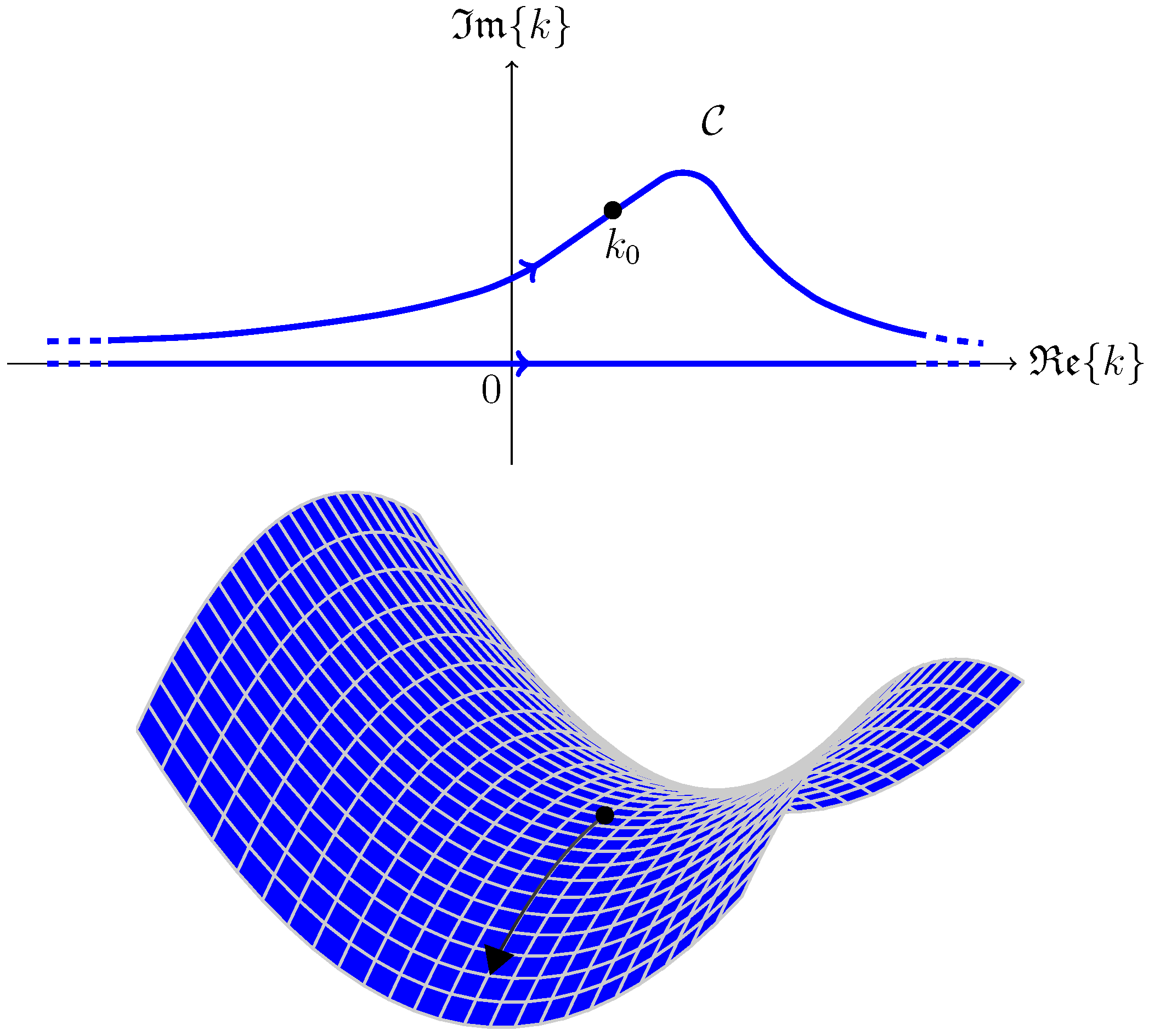
The large-t behaviour of such integrals can be established by invoking the steepest descent approximation [12,13]. The basis for this approximation is the following theorem.
Theorem 1.
Let us consider a function given by
where and are complex-valued functions of k. An approximation of at large-t can be expressed as
Here, is a saddle point of , namely a point such that the first derivative is zero; is such that all m-th order derivatives are zero for ; Γ is Euler’s gamma function.
The approximation is allowed if:
- 1.
- There exists a unique saddle point of , namely ;
- 2.
- There exists a path in the complex k plane that crosses along a line of steepest descent of ;
- 3.
- The region of the complex plane between path and the real axis, namely the line , does not contain any singularity or branch cut of (see Figure 2).
A proof of Theorem 1 can be found in many textbooks in applied mathematics, such as Bender and Orszag [12], or Ablowitz and Fokas [13], as well as in the recent paper by Barletta and Alves [8]. We point out that, in the neighbourhood of the saddle point , a line of steepest descent of is one where remains constant [8,12,13].
When function admits more than one saddle point, then the steepest descent approximation involves the sum of the contributions of different saddle points. In this case, there will be a leading contribution which comes from the term, or terms, with the highest value of .
On account of Theorem 1, the time dependence in the asymptotic expression of is given by the factor
Hence, if , we have
while, if , we have
If we apply Theorem 1 to detect the large-t asymptotic behaviour of functions and defined by Equation (22), we immediately conclude that function is identified with the coefficient and, on account of Equation (18), it is given by
We note that, for every and for every , is meromorphic with two simple poles at .
We are now ready to establish a criterion for detecting the onset of absolute instability, according to Definition 2 and Theorem 1:
- We find the saddle points by employing Equation (23) and by solving the algebraic equation .
- We check that the requirements stated in the thesis of Theorem 1 are satisfied by .
- We determine the threshold condition between an unbounded time growth of and and an exponential decay to zero, expressed by the algebraic equation .
Since is complex-valued, equation is in fact a pair of algebraic equations relative to the real and to the imaginary parts, respectively
where we used the shorthand and . For fixed , Equation (24) contains two unknowns, . Thus, solving these equations yields the saddle points . If, on the other hand, one aims to determine the saddle points and the corresponding value of , for prescribed , then one has to solve Equation (24) together with the algebraic equation . The latter can be written as
Equations (24) and (25) are the basis for a first screening of the saddle points . In fact, we can exclude those that yield a negative or a positive . These saddle points are not good candidates to the evaluation of the threshold of absolute instability. Among the remaining roots of Equations (24) and (25) one has to select the saddle point, or the saddle points, , such that the corresponding , given by Equation (25), is at its smallest and satisfies the requirements specified in the thesis of Theorem 1. By requiring that is at its smallest, we allow one to identify the least threshold to absolute instability, which is the physically meaningful one.
In particular, among the requirements specified in Theorem 1, one has to test whether there exists a path in the complex k plane that crosses the saddle point(s) along a direction of steepest descent, and such that the region of the plane between and the real axis, , does not contain any pole of . For the sake of brevity, this requirement is called analyticity requirement.
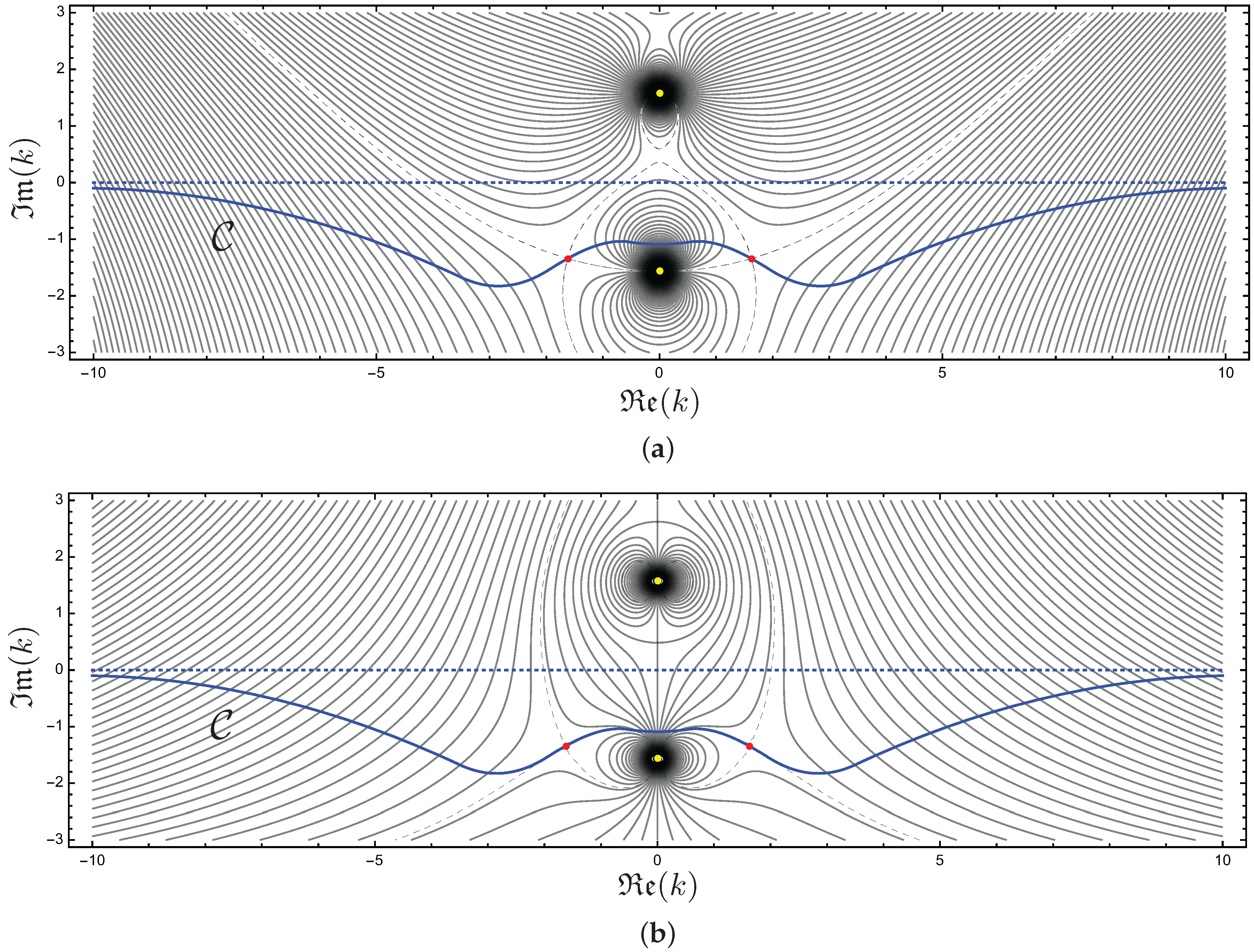
Example 1.
Let us test the whole procedure in the case . We first set and determine all the solutions of Equations (24) and (25). We obtain in fact six solutions,
The last pair of solutions is excluded because is negative. The first four solutions are acceptable because they satisfy the condition . Among them, we select the pair of solutions with the smallest , namely
We have to check if one can draw a path in the k plane that satisfies the analyticity requirement. This requirement can be tested by drawing the contour plots of and in the k plane, for , and . This allows a straightforward visualisation of the saddle points . Figure 3 reveals that the analyticity requirement is satisfied. The saddle points are evidenced as red points, while the yellow points are the poles . The qualitative line shows that it is possible satisfying the analiticity requirement, as this line can be continuously deformed to the real k axis without crossing any poles of . Thus, we conclude that are the relevant saddle points for the assessment of the onset of absolute instability, and that the threshold for absolute instability with is . A further note is for the qualitative sketch of path . Having drawn the contours of , it is very easy to detect the directions of steepest descent of . In fact, these directions are locally coincident with the contour line of which crosses the saddle point and connects the contour to the neighbouring contours with [8,12,13]. The extent to which path overlaps the contours , which cross the saddle points, can be expanded arbitrarily, thus matching the approximation defined by Theorem 1.
One may wonder whether inclusion of modes with or higher may yield saddle points corresponding to values of lower than . In fact, if we solve Equations (24) and (25) with and , we get
We don’t find any new candidates for the evaluation of , as all these solutions yield values of which are either negative or larger than . The same happens with , namely
We observe that modes with are sufficient to assess the correct value of . In fact, the general scaling behaviour of Equations (24) and (25) suggests that increases with n for large n, and thus enforces that one only needs to consider smaller values of n to determine the threshold of absolute instability.
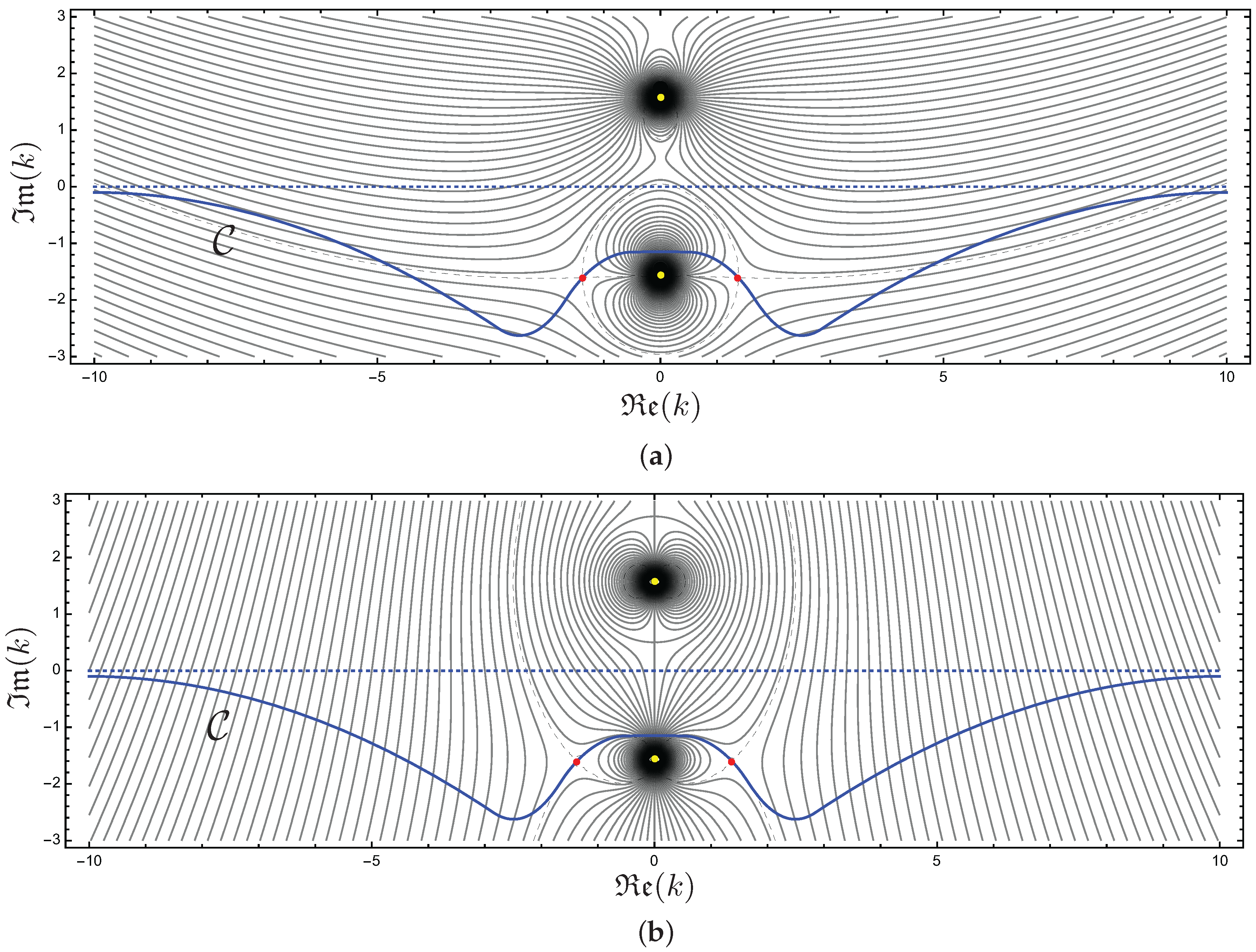
Example 2.
Things go much in the same manner if one considers . By setting , we get the solutions of Equations (24) and (25),
By the same reasoning employed in Example 1, we select the pair of solutions
Indeed, the saddle points satisfy the analyticity requirement and they can be used for the steepest descent approximation. This is readily inferred by inspecting Figure 4. We don’t catch any serious qualitative difference between Figure 3 and Figure 4. We mention that, once again, no role in assessing the threshold of absolute instability is played by modes with or higher. Thus, the conclusion is that the threshold of absolute instability, for , is .
4. Results
Examples 1 and 2 discussed in the preceding section lead us to the conclusion that the analysis of the transition from convective to absolute instability can be based on the solutions of the system of algebraic Equations (24) and (25).
Among the possible saddle points, we mention those with . These points are obtained for with , and they are given by
These saddle points are such that and thus they are, a priori, to be considered among the candidates for the evaluation of the threshold to absolute instability, . In fact, they appeared among the solutions discussed in Examples 1 and 2, with and 625, respectively. However, in both these examples, the saddle points expressed by Equation (26) did not contribute to the evaluation of . This conclusion is easily generalised by exploring other positive values of . We will further discuss these special saddle points later on.
Another remarkable class of saddle points is encountered in the special case . In this case, the solutions of are five,
In order to determine the threshold of absolute instability, only the last line of Equation(27) deserves attention, as the first and second lines express saddle points such that is real and either negative or positive, for every . Thus, only the last line is relevant to determine the threshold of absolute instability, that is the value of such that . By imposing the latter condition, one easily determines which, in turn, means . This result immediately leads us to the conclusion that, when , we have
Equation (28) means that, in the absence of a steady horizontal flow in the channel , the onset of convective instability means also the onset of absolute instability, and this happens when . This conclusion is completely obvious by relying on the physical meaning of the convective/absolute instability dichotomy.
The set of all saddle points of which satisfy the condition , for every , includes the whole imaginary axis, , with the exclusion of the origin and of the singularities . The imaginary axis, in fact, includes all saddle points defined by Equation (26) for all and . Moreover, is dense over closed curves in the complex k plane, defined implicitly by the polar equation,
where . A convenient visualization of the set is displayed in Figure 5a. The closed curve defined by Equation (29), represented in this figure, includes all saddle points in , with six exclusions denoted by yellow dots. These points are given by , where is singular, and by
The points defined by Equation (30) do not belong to because they do not satisfy the saddle point condition, , for any real values of . The blue dots in Figure 5a denote special elements of , namely the saddle points corresponding to and , that is . Figure 5b displays red curves joining all saddle points employed for the evaluation of at different Péclet numbers. The saddle points lying in the upper half of the k plane correspond to , while those in the lower plane are for . Up to this point, we just considered positive values of . Indeed, there is a perfect symmetry between the cases and , because whether the parallel flow is in the positive or negative x direction obviously cannot change the threshold of absolute instability. This means that, for a given , the value of is uniquely determined. The symmetry under a change of sign of is completely evident from Equation (23). In fact, a change of sign of is compensated by a change of sign of k, and this explains why the saddle points for and lie in two different halves of the k plane. Thus, in the following, we will always assume .
The same procedure described in Examples 1 and 2, with reference to and 50, can be extended to any . This allows one to evaluate the threshold for the onset of absolute instability, , for every given . A list of values of and of the corresponding saddle points are given in Table 1, with increasing values of . By extrapolating the data to the limit , one registers an unbounded, approximately linear, growth of with . The saddle points , with either a positive or a negative real part, change weakly when is very large. In fact, these tend to finite limits when , given by two of the four exclusions defined by Equation (30), with , namely
In the asymptotic regime where is very large, Table 1 suggests that tends to become a linear function of . The slope of this function, viz. , can be easily determined from Equation (23). In fact, if we write and we assume , then Equation (23) can be approximated as
The threshold value of absolute instability, , can be obtained by solving the saddle point condition, , with the constraint . We infer that the pertinent saddle points are those given by Equation (31), and that the value of is
Figure 6 illustrates the transition from convective to absolute instability. In particular, Figure 6a shows the threshold of absolute instability versus (black line). The lines with describe perturbations exponentially decaying in time. These lines lie below the threshold of absolute instability, and hence they correspond to . The reverse happens when , namely when the disturbance exponentially grows in time. In this case, the condition of absolute instability is satisfied and . Figure 6a also shows that, as increases, the transition from negative to positive values of becomes very steep, meaning that the change from to takes place, for a given , over a narrow interval of . Figure 6b displays the regions of stability, , convective instability, , and absolute instability, . This figure provides a clear indication of the increasing width of the convective instability region as increases, a feature quite evident also from the data reported in Table 1. The dashed line displayed in Figure 6b illustrates the good agreement, in a regime where is sufficiently large, between the numerical data for the threshold of absolute instability and the asymptotic behaviour defined by Equation (33).
A final comment is devoted to the class of saddle points defined by Equation (26) with and . There exists, in fact, a small interval where . In this interval, is larger than and lower than the threshold drawn in Figure 6. One may question if we have mistaken the evaluation of the threshold value of in this interval of . The answer is no, and the reason is as follows. For every Péclet number such that and for , there are two saddle points corresponding to . Both of them lie on the imaginary k axis: one is between the two singularities , while the other is below . Trying to draw a path , locally of steepest descent, that crosses both these saddle points is not possible without trapping the singularity within the region of space between and the real k axis. This feature precludes the application of the analyticity requirement prescribed by Theorem 1 or, stated differently, the saddle points defined by Equation (26) do not alter the evaluation of as reported in Figure 6. We refer the reader to Juniper et al. [14] for other examples where saddle points are to be excluded for violations of the analyticity requirement.
5. A Matter of Scaling
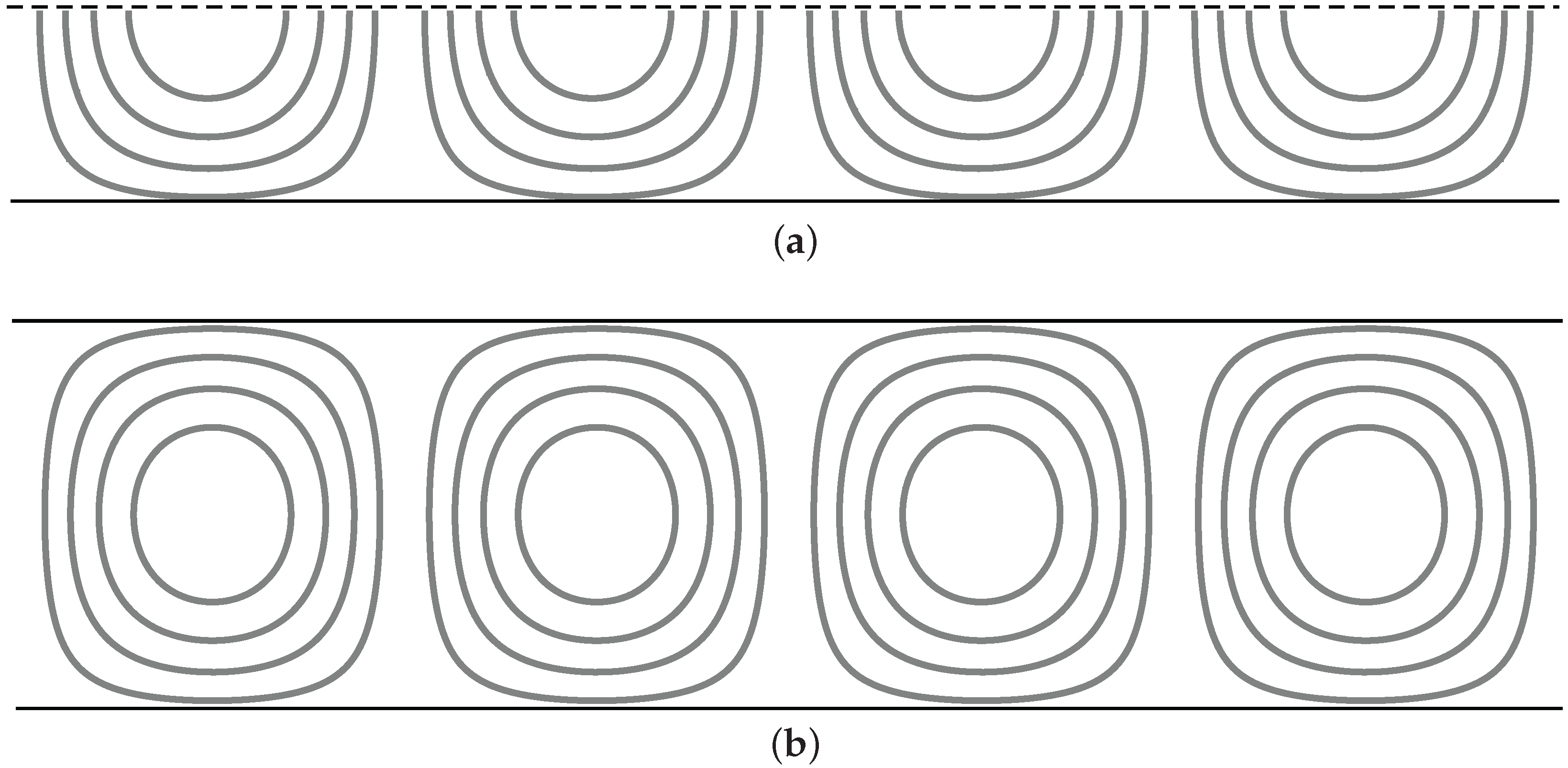
The analysis carried out so far is relative to a porous channel with an open upper boundary subjected to a uniform heat flux. A much more classic setup is one where both the lower and the upper boundaries are impermeable and isothermal. This setup is so classic that there is a name to denote it: the Horton-Rogers-Lapwood problem, also abbreviated with HRL problem [2]. The different boundary conditions considered in the HRL problem do not have any significant influence on the basic stationary flow across the channel. On the other hand, a sensible change emerges when expressing the Fourier modes of the perturbations, Equations (12)–(14). In fact, having an impermeable upper boundary with a uniform temperature implies that both and are zero at , so that Equation (14) is to be replaced by . This is the consequence of Neumann boundary conditions for and having been replaced by Dirichlet boundary conditions. If we limit our discussion to the modes, the only modes important for both the onset of convective and absolute instability, then we can reach a neat conclusion. With Dirichlet boundary conditions at we will have contour lines of with a sequence of rotating and counter-rotating cells, while Neumann boundary conditions have the effect that these cells are cut in the middle by the boundary : full cells in the former case and half cells in the latter (see Figure 7). Mathematically, the cells are exactly the same as they result from a product of sine functions in x and y. Therefore, it is not strange that the dispersion relation is exactly the same as in the HRL problem, and that the neutral stability condition (20) matches that for the HRL problem provided that k and are suitably scaled. Since the onset of convective instability comes about with half-cells, then the neutrally stable k for the HRL problem must be the double of that employed in Equation (20). Since Equation (6) shows that is proportional to , then doubling the channel thickness, to include the whole cells, implies that is turned into . Thus, Equation (21) immediately provides the critical values of k and for the HRL problem,
How does this scaling argument affect the data about the transition to absolute instability? We expect that we must multiply by 4 the numerical data of obtained in Section 4 to obtain those for the HRL problem. However, one must be careful with the value of . In fact, if is proportional to , is proportional to H as one may check on inspecting Equation (6). Thus, moving from our open boundary problem to the HRL problem, that is moving from the half cells to the full cells, or doubling the value of H, means multiplying the values of by a factor 2. To conclude, we can formulate the scaling as follows:
where we denoted with the threshold of absolute instability for our open boundary problem (data reported in Table 1), and with the threshold relative to the HRL problem.
That the scaling law (35) actually works can be easily checked by comparing the data obtained from Table 1, by applying Equation (35), with those reported in Barletta and Alves [8]. This comparison is done in Table 2, for a few sample values of . The agreement is complete within six significant figures.
6. Going Three-Dimensional
A question arises about the behaviour of the flow when the assumption of a very small spanwise width, L, is relaxed. In this case, a value of L comparable with H or larger implies a significant functional dependence on z of the velocity, pressure and temperature fields. One may envisage a lateral confinement along the spanwise z direction with adiabatic impermeable sidewalls. The basic solution (3) still holds, except that one must also specify that the z component of velocity is zero and, as a consequence, also the z component of the pressure gradient is zero. The analysis of small-amplitude perturbations is to be carried out on three-dimensional grounds. Hence, a streamfunction formulation is out of the question, while a pressure formulation is possible,
Here, the dimensionless coordinate z is defined coherently with , by adopting the same scale H. We have , where . Instead of Equation (10), the boundary conditions are now written as
We now introduce the Fourier transforms,
with the inverse transforms given by
We can now separate the dependence on y and z, in analogy with Equation (13),
where is still given by Equation (14), while . Definitions 1 and 2 are easily generalised to
Definition 3.
The parallel flow given by Equation (3) is convectively unstable if there exist and such that
Definition 4.
The parallel flow given by Equation (3) is absolutely unstable if, for every , there exists such that
By applying the Fourier transform to Equation (36), one obtains
Equation (41) can be solved by writing
with the dispersion relation now given by
The condition for the onset of convective instability is formulated by setting and , so that Equation (43) yields
The lowest value of leading to convective instability is obtained with ,
which replaces the neutral stability condition (20). By minimising , one obtains the critical value when
There are several solutions of Equation (46), depending on the value of the aspect ratio . For instance, if , there is just one possible solution: with . This means that, with , the onset of convective instability happens when z-independent Fourier modes are activated, namely modes having and , in agreement with the two-dimensional analysis, Equation (21). Things get more and more complicated when . If , then two Fourier modes become convectively unstable when exceeds the critical value . One is the z-independent mode and the other one is
The mode is three-dimensional, that is, z-dependent. Further three-dimensional Fourier modes become convectively unstable at the critical condition , if .
The three-dimensional analysis of the transition to absolute instability is not to be based on Equation (23), but on its generalisation implied by Equation (43), namely
By relying on Definition 4, the transition to absolute instability has just the same features described with the two-dimensional analysis if the Fourier integrals calculated with become time-growing at Rayleigh numbers lower than those for the integrals calculated with . If this is the case, the transition to absolute instability happens with purely two-dimensional modes, and the analysis carried out in the preceding sections does not need to be modified. In order to illustrate how things go when modes with are included in the analysis, we will reconsider the cases examined in Examples 1 and 2.
Example 3.
We assume and , since modes do not contribute to the two-dimensional analysis. By considering either and a finite , or and , we have . In this case, the saddle points of such that are just the same as those gathered in the two-dimensional analysis, namely
with yielding the lowest greater or equal than , and thus leading to the result .
If we now consider three-dimensional modes with , our solutions will depend on .
If we set then the saddle points of such that are
not providing any candidate for the evaluation of .
If we set then the saddle points of such that are
The conclusion is just the same as for . If we now trace the behaviour of the saddle points by gradually increasing up to 50, we obtain that there is no saddle point yielding a value of larger than , but lower than . Interestingly enough, we note that with our saddle points are
These saddle points are not much different from those obtained with the two-dimensional analysis, namely with either or and . We note that there is one extra saddle point with a very large Rayleigh number. This point disappears when the limit is taken.
The conclusion to be drawn by inspecting the behaviour of the saddle points with and gradually increasing is that the evaluation of the threshold value of for the transition to absolute instability coincides with that relative to the two-dimensional analysis, namely . No difference is made if one considers or larger. In fact, due to the definition of , modes with and a given yield the same , and hence the same saddle points, as modes with and a suitably smaller .
Example 4.
A behaviour much similar to that described in Example 3 is observed for . By setting and , the saddle points for the two-dimensional analysis are (see also Example 2),
From these saddle points, the conclusion drawn in Example 2 is that the threshold for absolute instability is . If three-dimensional modes with are now included in our analysis, we can keep track of the saddle points obtained by starting with and gradually increasing up to 50. We do not find any saddle points of such that whose corresponding value of is both larger than and lower than . In particular, for we obtain
A set of saddle points not much different from those obtained with the two-dimensional analysis. We note that the second saddle point with a value of around 625 appears only for larger values of . However, we know that this solution does not influence the evaluation of .
Exactly as in Example 3, we can conclude that the three-dimensional analysis does not modify in any way our evaluation of .
The features of the three-dimensional analysis, described in Examples 3 and 4, can be easily generalised to other Péclet numbers. The general rule is that the three-dimensional analysis does not change the threshold values of absolute instability, , evaluated through a purely two-dimensional analysis.
Obviously, a remarkable situation is , already discussed within the two-dimensional analysis. In this case, the solutions of are five,
The second line of Equation (48) can be skipped as it never gives raise to a vanishing . For every n, both the first and the third line of Equation (48) yield for , provided that is an integer multiple of 2 and l is suitably chosen. For other values of , the lowest value of leading to is given by the third line of Equation (48). Thus, whatever is the value of , the threshold of absolute instability is . This means that, also for =0, the three-dimensional analysis leads exactly to the same results obtained by the two-dimensional analysis. Just the same behaviour was reported, with reference to a similar flow regime, by Delache et al. [15].
7. Conclusions
The analysis of convective and absolute instability has been carried out for the stationary flow in a porous horizontal channel. The lower boundary of the channel has been considered as impermeable and isothermal, while the upper boundary has been modelled as open to an external tangential flow and uniformly cooled. The setup is one of heating from below, so that the kind of instability is Rayleigh-Bénard. The concepts of convective and absolute instability have been reviewed and the detailed procedure to assess the conditions for both types of instability has been described.
The analysis of instability has been initially formulated by a two-dimensional scheme, in order to keep the mathematical difficulties at their lowest. Then, the study has been extended to three-dimensional perturbations thus assessing the validity of the two-dimensional formulation.
The main results of the analysis performed in this paper are the following:
- The concepts of convective and absolute instability can be rigorously defined by applying the Fourier transform method to solve the perturbation equations. The Fourier transformed variable is the coordinate along the streamwise direction.
- The assessment of convective instability just deals with the time-growth, or time-decay, of the Fourier transformed perturbations. The study of the absolute instability, on the other hand, is focussed on the large-time behaviour of the perturbations themselves.
- The need to track the large-time behaviour of the perturbations, mathematically of the inverse Fourier transforms, leads to the central role played by the steepest-descent approximation.
- The two-dimensional analysis of convective instability does not yield a condition of convective instability different from that obtained with a three-dimensional analysis. The only difference is in the modes leading to the critical value of the Rayleigh number for the onset of convective instability, . The number of unstable Fourier modes at gradually increases as the spanwise-to-vertical aspect ratio of the channel cross-section, , increases.
- The onset of absolute instability occurs at a Rayleigh number , where the equality holds if and only if the Péclet number, , is zero. The threshold of absolute instability, , is a monotonic increasing function of . When , becomes approximately a linear function of .
- For a given , the threshold value of absolute instability, , obtained by a two-dimensional analysis coincides with that obtained by a three-dimensional analysis.
- A suitable scaling of the parameters turned out to map the study carried out in this paper to the analogous study of the Horton-Rogers-Lapwood problem, not only for the results of the convective instability study, but also for the analysis of the transition to absolute instability.
Author Contributions
This is joint research by the authors.
Conflicts of Interest
The authors declare no conflict of interest.
References
- Drazin, P.G.; Reid, W.H. Hydrodynamic Stability, 2nd ed.; Cambridge University Press: New York, NY, USA, 2004. [Google Scholar]
- Nield, D.A.; Bejan, A. Convection in Porous Media, 5th ed.; Springer: New York, NY, USA, 2017. [Google Scholar]
- Brevdo, L.; Bridges, T.J. Local and global instabilities of spatially developing flows: Cautionary examples. Proc. R. Soc. Lond. A Math. Phys. Eng. Sci. 1997, 453, 1345–1364. [Google Scholar] [CrossRef]
- Huerre, P.; Monkewitz, P.A. Absolute and convective instabilities in free shear layers. J. Fluid Mech. 1985, 159, 151–168. [Google Scholar] [CrossRef]
- Brevdo, L. Convectively unstable wave packets in the Blasius boundary layer. ZAMM J. Appl. Math. Mech. Z. Angew. Math. Mech. 1995, 75, 423–436. [Google Scholar] [CrossRef]
- Lingwood, R.J. On the application of the Briggs’ and steepest-descent methods to a boundary-layer flow. Stud. Appl. Math. 1997, 98, 213–254. [Google Scholar] [CrossRef]
- Suslov, S.A. Numerical aspects of searching convective/absolute instability transition. J. Comput. Phys. 2006, 212, 188–217. [Google Scholar] [CrossRef]
- Barletta, A.; Alves, L.S. de B. Absolute instability: A toy model and an application to the Rayleigh-Bénard problem with horizontal flow in porous media. Int. J. Heat Mass Transf. 2017, 104, 438–455. [Google Scholar] [CrossRef]
- Brevdo, L.; Bridges, T.J. Absolute and convective instabilities of spatially periodic flows. Philos. Trans. R. Soc. Lond. A Math. Phys. Eng. Sci. 1996, 354, 1027–1064. [Google Scholar] [CrossRef]
- Rees, D.A.S. The stability of Darcy-Bénard convection. In Handbook of Porous Media; Vafai, K., Hadim, H.A., Eds.; CRC Press: New York, NY, USA, 2000; Chapter 12; pp. 521–558. [Google Scholar]
- Barletta, A. Thermal instabilities in a fluid saturated porous medium. In Heat Transfer in Multi-Phase Materials; Öchsner, A., Murch, G.E., Eds.; Springer: New York, NY, USA, 2011; pp. 381–414. [Google Scholar]
- Bender, C.M.; Orszag, S.A. Advanced Mathematical Methods for Scientists and Engineers I; Springer: New York, NY, USA, 1999. [Google Scholar]
- Ablowitz, M.J.; Fokas, A.S. Complex Variables: Introduction and Applications; Cambridge University Press: Cambridge, UK, 2003. [Google Scholar]
- Juniper, M.P.; Hanifi, A.; Theofilis, V. Modal stability theory. Appl. Mech. Rev. 2014, 66, 024804. [Google Scholar]
- Delache, A.; Ouarzazi, M.N.; Combarnous, M. Spatio-temporal stability analysis of mixed convection flows in porous media heated from below: Comparison with experiments. Int. J. Heat Mass Transf. 2007, 50, 1485–1499. [Google Scholar] [CrossRef]
Figure 1.
A sketch of the porous channel, of the flow geometry and of the boundary conditions.
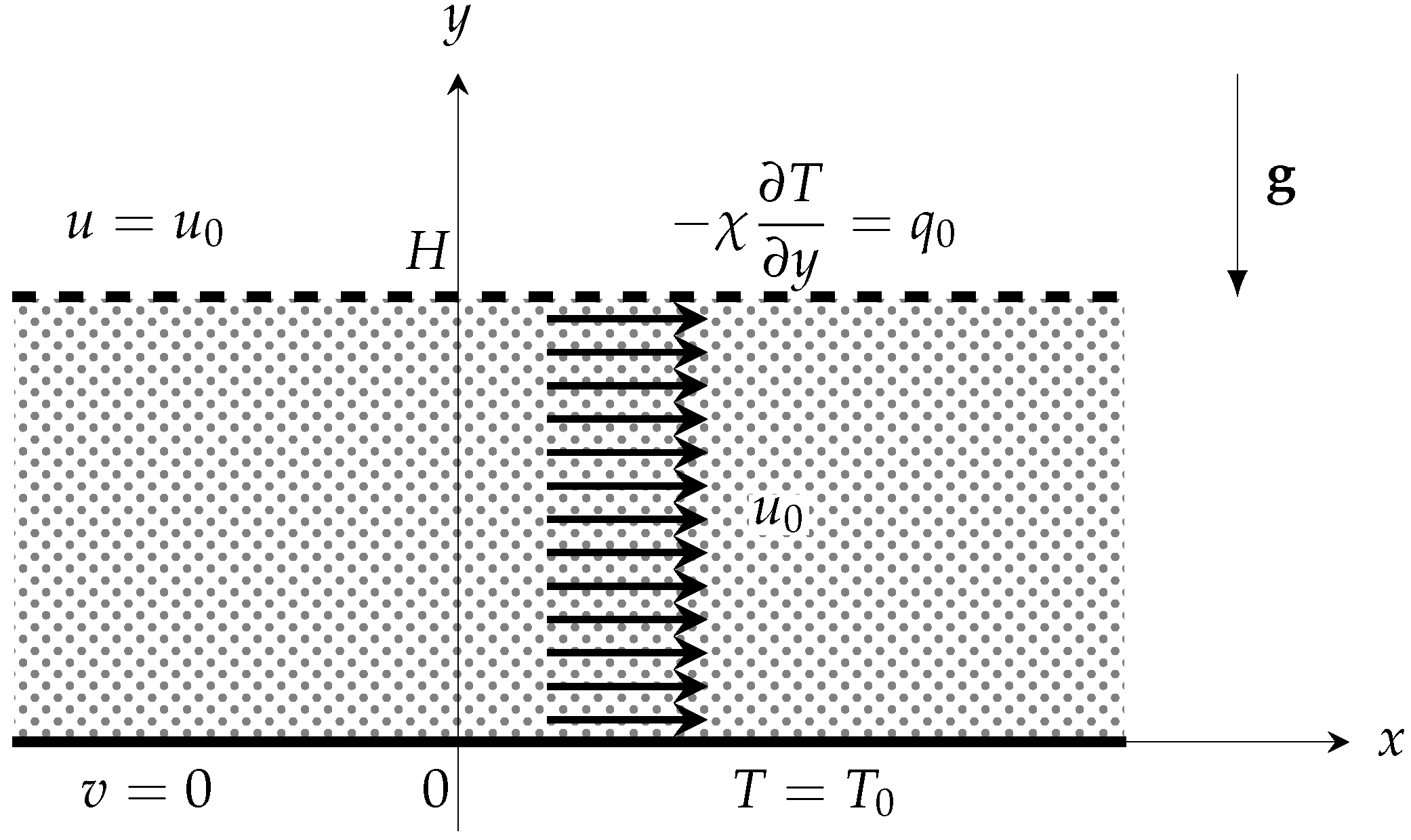
Figure 2.
A sketch of the saddle point of in the complex k plane and of the line of steepest descent.
Figure 2.
A sketch of the saddle point of in the complex k plane and of the line of steepest descent.

Figure 3.
Threshold of absolute instability, , with , : (a) contours of in the complex k plane; (b) contours of in the complex k plane. The red dots denote the saddle points ; the yellow dots denote the singularities ; the black dashed contours are relative to ; the blue solid line is a possible path that crosses the saddle points along a direction of steepest descent; the dotted blue line is the real axis, .

Figure 4.
Threshold of absolute instability, , with , : (a) contours of in the complex k plane; (b) contours of in the complex k plane. The red dots denote the saddle points ; the yellow dots denote the singularities ; the black dashed contours are relative to ; the blue solid line is a possible path that crosses the saddle points along a direction of steepest descent; the dotted blue line is the real axis, .

Figure 5.
(a) Curve in the complex plane representing all possible saddle points of , with , for all real values of , and for all natural numbers n. Yellow dots denote exclusions from the set of saddle points, while blue dots denote the saddle points with ; (b) Curve in the complex k plane including all saddle points employed to evaluate with either (lower plane) or (upper plane). The dashed blue line denotes the real axis, with blue dots denoting the case , and yellow dots denoting the limiting cases .
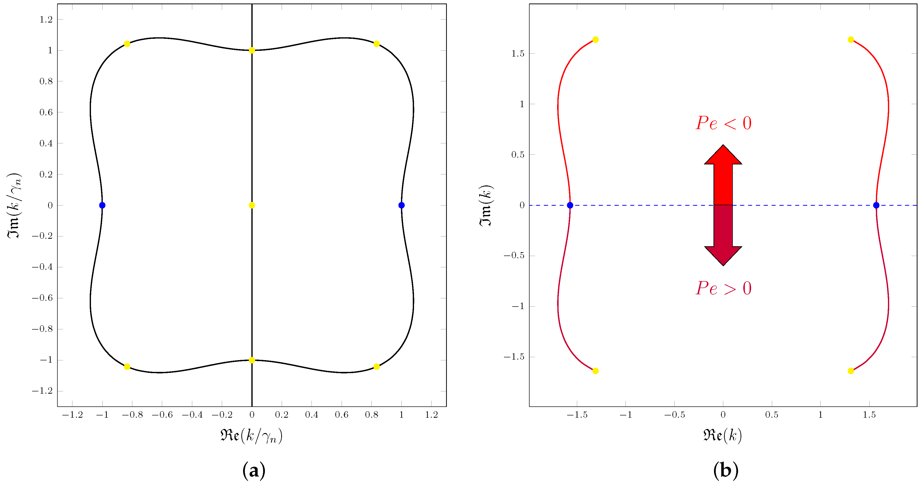
Figure 6.
(a) Transition to absolute instability: values of versus obtained for the saddle points with increasing values of , from negative to positive. The black line yields the threshold of absolute instability, namely ; (b) Map of the regions in the parametric plane relative to stability, convective instability, and absolute instability; the dashed line shows the asymptotic behaviour described by Equation (33).
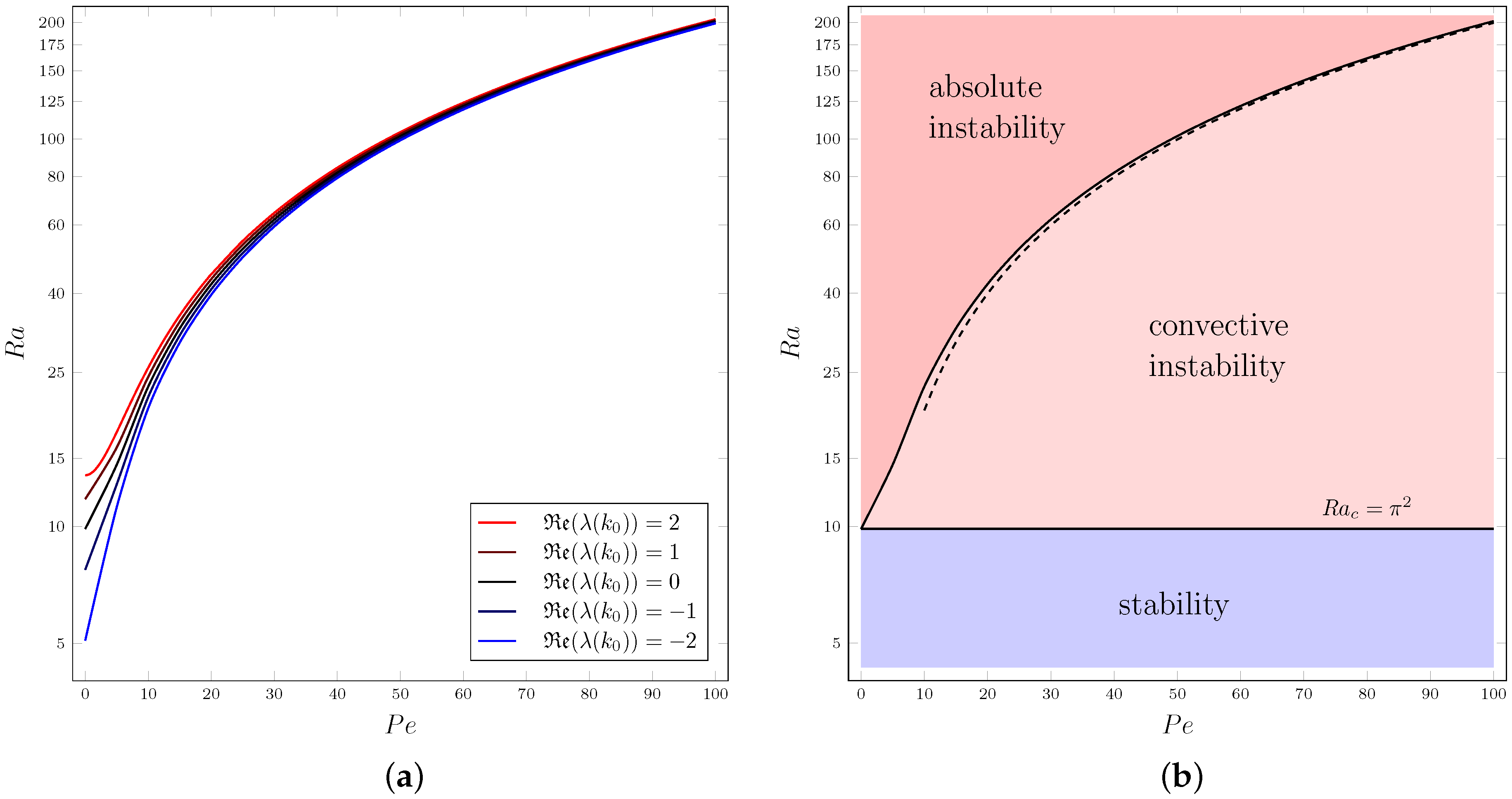
Figure 7.
Scaled convection streamlines of the perturbations for: (a) the open upper boundary problem; (b) the HRL problem.
Figure 7.
Scaled convection streamlines of the perturbations for: (a) the open upper boundary problem; (b) the HRL problem.


Table 1.
Threshold values of for the onset of absolute instability with increasing values of . The relevant saddle points for the evaluation of are reported.
Table 1.
Threshold values of for the onset of absolute instability with increasing values of . The relevant saddle points for the evaluation of are reported.
| 0 | ||
| 5 | 14.4509 | |
| 10 | 22.9882 | |
| 15 | 32.4868 | |
| 20 | 42.2506 | |
| 25 | 52.1103 | |
| 30 | 62.0136 | |
| 35 | 71.9402 | |
| 40 | 81.8806 | |
| 45 | 91.8298 | |
| 50 | 101.7851 | |
| 55 | 111.7446 | |
| 60 | 121.7072 | |
| 65 | 131.6722 | |
| 70 | 141.6391 | |
| 75 | 151.6074 | |
| 80 | 161.5768 | |
| 85 | 171.5472 | |
| 90 | 181.5183 | |
| 95 | 191.4901 | |
| 100 | 201.4625 | |
© 2017 by the authors. Licensee MDPI, Basel, Switzerland. This article is an open access article distributed under the terms and conditions of the Creative Commons Attribution (CC BY) license (http://creativecommons.org/licenses/by/4.0/).
Share and Cite
MDPI and ACS Style
Barletta, A.; Celli, M. Convective to Absolute Instability Transition in a Horizontal Porous Channel with Open Upper Boundary. Fluids 2017, 2, 33. https://doi.org/10.3390/fluids2020033
AMA Style
Barletta A, Celli M. Convective to Absolute Instability Transition in a Horizontal Porous Channel with Open Upper Boundary. Fluids. 2017; 2(2):33. https://doi.org/10.3390/fluids2020033
Chicago/Turabian StyleBarletta, Antonio, and Michele Celli. 2017. "Convective to Absolute Instability Transition in a Horizontal Porous Channel with Open Upper Boundary" Fluids 2, no. 2: 33. https://doi.org/10.3390/fluids2020033