The Impact of Horizontal Resolution on Energy Transfers in Global Ocean Models


Atmospheric, Oceanic and Planetary Physics, Department of Physics, University of Oxford, Oxford OX1 3PU, UK
*
Author to whom correspondence should be addressed.
Fluids 2017, 2(3), 45; https://doi.org/10.3390/fluids2030045
Submission received: 15 July 2017
/
Revised: 15 August 2017
/
Accepted: 24 August 2017
/
Published: 28 August 2017
(This article belongs to the Collection Geophysical Fluid Dynamics)
Abstract
:The ocean is a turbulent fluid with processes acting on a variety of spatio-temporal scales. The estimates of energy fluxes between length scales allows us to understand how the mean flow is maintained as well as how mesoscale eddies are formed and dissipated. Here, we quantify the kinetic energy budget in a suite of realistic global ocean models, with varying horizontal resolution and horizontal viscosity. We show that eddy-permitting ocean models have weaker kinetic energy cascades than eddy-resolving models due to discrepancies in the effect of wind forcing, horizontal viscosity, potential to kinetic energy conversion, and nonlinear interactions on the kinetic energy (KE) budget. However, the change in eddy kinetic energy between the eddy-permitting and the eddy-resolving model is not enough to noticeably change the scale where the inverse cascade arrests or the Rhines scale. In addition, we show that the mechanism by which baroclinic flows organise into barotropic flows is weaker at lower resolution, resulting in a more baroclinic flow. Hence, the horizontal resolution impacts the vertical structure of the simulated flow. Our results suggest that the effect of mesoscale eddies can be parameterised by enhancing the potential to kinetic energy conversion, i.e., the horizontal pressure gradients, or enhancing the inverse cascade of kinetic energy.
1. Introduction
Ocean currents and eddies have systematically less kinetic energy (KE) in low-resolution simulations than high-resolution simulations [1,2]. Less energetic currents and eddies can cause biases in e.g., the strength of overturning circulations [3], oceanic heat uptake [4], and mixed-layer depth [5] as well as model drifts [6]. To understand what sets the energy levels in ocean models at different horizontal resolutions and what parameterisations may be needed, we must understand how KE is transfered between length scales. A key length scale for the transfer of KE in the ocean is the first baroclinic Rossby radius (hereafter just “Rossby radius”), which is the characteristic length scale at which perturbations in the first baroclinic mode become geostrophically balanced. On scales larger than the Rossby radius, the ocean behaves, to first order, as a quasi two-dimensional turbulent flow due to the strong stratification. A prominent feature of two-dimensional turbulence is the “inverse cascade”, where nonlinear interactions transfer KE from smaller to larger spatial scales [7]. This is unlike the “forward cascade” in three-dimensional turbulence, where KE is transferred from larger to smaller scales and then dissipated [8]. For a two-layer flow, Salmon and Scott, et al. [9,10] showed a simplified view of the transfer of KE as a function of length scale. The baroclinic mode exhibits a forward cascade of potential energy (PE) from large scales to the Rossby radius scale, , where there is conversion from PE to KE. Some of the baroclinic KE is then transfered to barotropic KE, often called “barotropisation” [11] and its efficiency depends on on several factors such as stratification and bottom drag [12,13,14,15]. Both the barotropic and baroclinic modes exhibit an inverse cascade of KE from the Rossby radius scale to larger scales [10,16], while there is a forward cascade of KE from the Rossby radius toward smaller scales [17]. The magnitude of large-scale KE in an ocean model thus depends on the ability of the model to resolve the Rossby radius, typically 10–50 km in midlatitudes, in order to produce the correct transfer of KE and PE between large scales (∼) and mesoscale eddies. Non-eddying ocean models, e.g., with (∼) horizontal resolution, often use an eddy-parameterisation scheme such as [18] (hereafter GM) to account for unresolved eddy processes. However, while such parameterisations imitate tracer fluxes by eddies, they do not include the inverse cascade of KE. As a result, the Gulf Stream, Antarctic Circumpolar Current (ACC), and Kuroshio are generally weak in low-resolution models. Eddy-permitting, ∼ (∼) horizontal resolution, and eddy-resolving models, ∼– (∼5–) horizontal resolution, resolve the Rossby radius in midlatitudes and therefore simulate more realistic energy spectra and fluxes than non-eddying models [19,20]. However, in eddy-permitting models, the horizontal resolution is close to the Rossby radius in midlatitudes, and thus conversion of PE to KE and the inverse cascade of KE occur near the grid scale where the effects of viscosity often dominates [1,20]. Thus, eddy-permitting models generally underestimate the overall KE as well as the magnitude of energy transfers between length scales while eddy-resolving models are more realistic.
As eddy-permitting ocean simulations often struggle to reproduce the strong currents and eddy activity in regions such as the Gulf Stream, recent years have seen much development in parameterising the effect of unresolved scales in eddy-permitting ocean models. One method is to make viscosity scale-aware in order to make the model less viscous while still ensuring numerical stability [21,22,23]. Other methods focus on augmenting the weak inverse cascade of KE in eddy-permitting models [19,20,24,25]. In addition, horizontal pressure gradients, i.e., the conversion from PE to KE, can be intensified by accounting for unresolved temperature and salinity fluctuations in the nonlinear equation of state [26]. A few studies have analysed the spectral properties of KE and PE in global ocean models. Schloesser and Eden [27] studied the North Atlantic and found an inverse cascade of KE and a forward cascade of PE. Arbic, et al. [1] used a very high-resolution model, (∼), and found that both temporal and spatial filtering can introduce an artificial forward cascade of KE at the smallest resolved scales. Chemke, et al. [15] used an ocean state estimate to analyse the barotropic KE budget and understand how barotropisation scales with properties of the flow (e.g., stratification, vertical velocity shear) following the [12] theory. In this paper, we will investigate why varying horizontal resolution changes the amount of KE and if this is true for several regions with strong currents and eddy activity in the world oceans. We will use three simulations with the nucleus for european modelling of the ocean (NEMO) ocean model at non-eddying (), eddy- permitting (), and eddy-resolving resolution () to diagnose the differences. We present the KE budget in Section 2, and describe the model simulations in Section 3. We will, in Section 4, show that horizontal resolution and the necessary horizontal viscosity exerts a strong control on the KE transfers between length scales, the relative importance of terms in the KE budget, and the partitioning of KE into barotropic and baroclinic modes. We will lastly, in Section 5, summarise our results and discuss possible routes for parameterising unresolved energy transfers.
2. Theory
2.1. Kinetic Energy in Physical Space
The 2D KE equation in our ocean model, NEMO ([28], see Section 3 for further details), can be summarised as
where
is the horizontal velocity, w is the vertical velocity, p is pressure, and is the reference density. The horizontal gradient operator is denoted and the vertical gradient is . The ocean is forced at the surface by wind input, given by the vertical derivatives of zonal and meridional components of wind stress, . Dissipation at the ocean lower boundary is done using quadratic bottom drag with a coefficient given by , where is the background turbulent kinetic energy and is a non-dimensional parameter. Horizontal and vertical viscosity are set by the respective coefficients and . The viscosity operator uses for non-eddying simulations and eddying simulations, respectively, as is commonly done in ocean simulations [29,30,31].
We identify the terms in Equation (1) as kinetic energy for the horizontal velocity components , horizontal nonlinear interactions N, vertical nonlinear interactions , wind forcing W, bottom drag D, horizontal pressure work (which is responsible for the conversion between PE and KE) P, horizontal viscosity V, and vertical viscosity . We make the approximation that and , where H is a reference depth set to either or depending on the region studied (as explained in Section 3). We calculate the PE to KE conversion using the pressure gradient term above to be consistent with the underlying NEMO calculations (note that it is different from e.g., [17] who used , where b is buoyancy). We perform these calculations on results from an idealised double-gyre simulation with parameter settings similar to ORCA025 and compare to the online tendencies from the model, and find only very small differences (see Section 3). When calculating KE budgets, we ignore vertical transfer of momentum, , and vertical viscosity, . These terms are much smaller than all other terms and do not contribute to the 2D KE budget in real or spectral space. We will also ignore bottom drag, D, when focusing on the upper ocean.
2.2. Two-Layer Turbulence
As described in Section 3, we will average the ocean model data onto two layers, and , separated at a depth , to partition KE to the barotropic and baroclinic modes. With this approach, the baroclinic mode will encapsulate all baroclinic modes into one. We denote the velocity of the barotropic mode as and the velocity for the baroclinic mode as where the baroclinic velocities are defined in both the upper layer and lower layer. Similarly to [15], we define the velocity in the two modes as
where is the total ocean depth. Subscripts 1 and 2 denote the upper and lower layers, respectively.
The full derivation of the barotropic and baroclinic KE budgets is presented in Appendix A. In this paper, we will mainly focus on the nonlinear interactions and barotropisation in the barotropic and baroclinic KE budgets. These are identified as (barotropic self-interactions) and (barotropisation), (baroclinic self-interactions), and (“catalytic” term). As described in Appendix A, and following [16], we add the “catalytic” baroclinic KE nonlinear interactions, , to the baroclinic self-interaction to get the total baroclinic nonlinear term. In our calculations, the catalytic term has a very similar structure to the baroclinic self-interaction, so adding them enhances the total baroclinic KE flux. We will ignore the “barotropic stirring” term as this is small in the baroclinic KE budget. Scott, et al. [16] argues that the barotropic stirring term in the baroclinic KE budget corresponds to the barotropisation term in the barotropic KE budget. We also note that the baroclinic self-interaction, , is non-zero only when the two layers have different thickness [16].
2.3. Kinetic Energy in Spectral Space
In order to study the KE budget as a function of length scales, we do a Fourier transform in the horizontal directions:
where are zonal and meridional wavenumbers and curly braces, { }, denotes the Fourier transformed variable. We make similar Fourier transforms of velocity, wind forcing, pressure and their respective gradients to get the time-averaged KE budget in spectral space. We obtain the budget for the KE power spectrum by integrating over wavenumbers
where , and denotes complex conjugates. Square brackets, is a vertical average. We only do a vertical average over the upper ocean, i.e., or , as defined in Section 3. In the above integral, we assume that the flow is isotropic and proceed to use only the isotropic wavenumber, . This gives us the budget
where denotes the integral of a transfer which are given by
where are surface velocities, are bottom velocities, is a vertical average as before and is a time average. The time average is taken over the entire simulation length, 1 January 1979 to 31 December 2009. As previously stated, we ignore vertical momentum transfer, , and vertical viscosity, , as they are relatively small terms. We also ignore bottom drag, D, when studying the upper ocean. Note that we evaluate gradients in space before making the Fourier transform, e.g., we calculate , then Fourier transform to get and then multiply by to get the contribution to KE. This is different from e.g., [10], where gradients are evaluated in spectral space from the Fourier transformed velocities. Our method also differs from Aluie, et al. [32], which may be more accurate.
In the case of PE conversion to KE near the Rossby radius wavelength, , and a KE flux from toward larger scales of as shown by [33], we would expect and with the extrema between and . Important scales for interpreting the spectra and fluxes of KE are the energy-containing scale, defined as the mean wavenumber weighted by energy, i.e.,
and the first baroclinic Rossby radius of deformation
where [34]. Typically, in ocean mid-latitudes, the energy-containing scale is ∼ [34] and the Rossby radius is 10–50 [34]. In our paper, we will calculate the Rossby radius for each grid cell in our eddy-resolving simulation (ORCA0083) in each region, and then present the regional average. As we will show later, is approximately the wavenumber at which the KE spectrum, , as well as and reach their extremes.
We make similar transforms for the baroclinic and barotropic KE and the nonlinear terms. The barotropic and baroclinic KE are
where square brackets denote a vertical average over the two layers and as before.
We integrate as in Equation (5) to get power spectra and as well as spectral fluxes. The time-averaged barotropic and baroclinic KE budgets are thus
The full derivation of these terms can be found in the Appendix. In this paper, we will focus on barotropic nonlinear interactions, , baroclinic nonlinear interactions, and barotropisation, .
3. Model Data
We use model data from realistic configurations of the 3D NEMO ocean model [28] with three different horizontal resolutions. Data are available as five-day averages, which is high enough temporal resolution to resolve most of the mesoscale eddy activity. The model simulations are the same as used by [35]. The only differences between our three different configurations are the horizontal resolution, horizontal viscosity, , tracer diffusion, and time step [28]. All configurations use a NEMO 3.6 ocean model with the LIM2 sea-ice model, and are forced at the surface with ERA-Interim [36] wind and buoyancy forcing for 1979–2009. All three configurations all have 75 vertical levels where the volume of a column can vary in time. We ignore this variation in layer thickness, but the associated error is on the order of . Bottom topography is represented with partial steps. All configurations use Laplacian iso-neutral tracer diffusion to represent sub-grid scale tracer mixing. Vertical viscosity, , is calculated from a turbulent kinetic energy (TKE) closure scheme, with a minimum background value given in Table 1. A quadratic bottom drag is applied in all configurations. The time step and horizontal viscosity are different at different horizontal resolution in order to ensure numerical stability. Similarly, the tracer diffusion is increased at coarser resolution so that the resulting fields are smooth. In ORCA025 and ORCA0083, the order of the horizontal viscosity operator is increased in order to make the dissipation more concentrated to the grid scale [21,29]. Eddy fluxes of heat and salt are parameterised in ORCA1 using the GM scheme [18], but not at finer resolution since eddies are, at least partially, resolved in ORCA025 and ORCA0083 and thus eddy tracer fluxes are already explicitly simulated. However, in simulations of high-latitude or shelf processes, the GM scheme could be beneficial even at resolution and finer [2,37]. The settings used for the ocean model configurations are summarised in Table 1.
To decompose the KE and spectral fluxes of KE into barotropic and baroclinic modes, we average our global ocean model data onto two vertical levels separated at . This allows us to calculate the KE and spectral fluxes in the barotropic mode, leaving the remainder to be the sum of all baroclinic modes. The baroclinic mode will be dominated by the first baroclinic mode, as most of the KE is in the barotropic or the first baroclinic mode [38]. The reason for averaging the velocities onto only two levels is to avoid depths intersected by bathymetry, where many grid cells become invalid causing large errors in the spectral transform. The separation depth is set to for the ACC and Malvinas regions, and for the Kuroshio, Gulf Stream and East Pacific regions based on the vertical structure of velocity and stratification in the different regions. While our choices of are subjective, we have experimented with different for the different regions and found that while the absolute values can change, the results of this study are unchanged. The depth in the Kuroshio is shown as a black dashed line in Figure 1.
The KE budget, which is calculated using five-day averages, is not expected to be exactly balanced. The total imbalance in the KE budgets (Equation (6)) presented later is of the order in all regions studied. This is partly because we are not including all terms in our calculations, e.g., vertical viscosity, bottom drag, vertical momentum transfer, etc., although they are relatively small terms. The spectral flux of vertical momentum transfer is on the order of , which is an order of magnitude less than the other terms, and vertical viscosity is even smaller. The imbalance in the KE budget is also due to the interpolation we use to calculate the spectral fluxes, as well as the fact that we are only diagnosing the upper ocean, i.e., down to or , except when we average onto two layers. We have repeated our calculations on an idealised, flat-bottomed, double-gyre configuration of NEMO with parameters similar to the ORCA025 simulation. Comparing our calculated spectral fluxes based on five-day averages with the exact online tendencies from the model, we found some small differences that were mostly due to interpolation (As an example, in physical space, KE contribution from zonal wind forcing is , evaluated at the U-point and then interpolated to the T-point. In spectral space, u and are interpolated to the T-point, then Fourier transformed, and the KE contribution is . Hence, the two terms will not be exactly equal.).
4. Results
4.1. Kinetic Energy (KE) in Physical Space
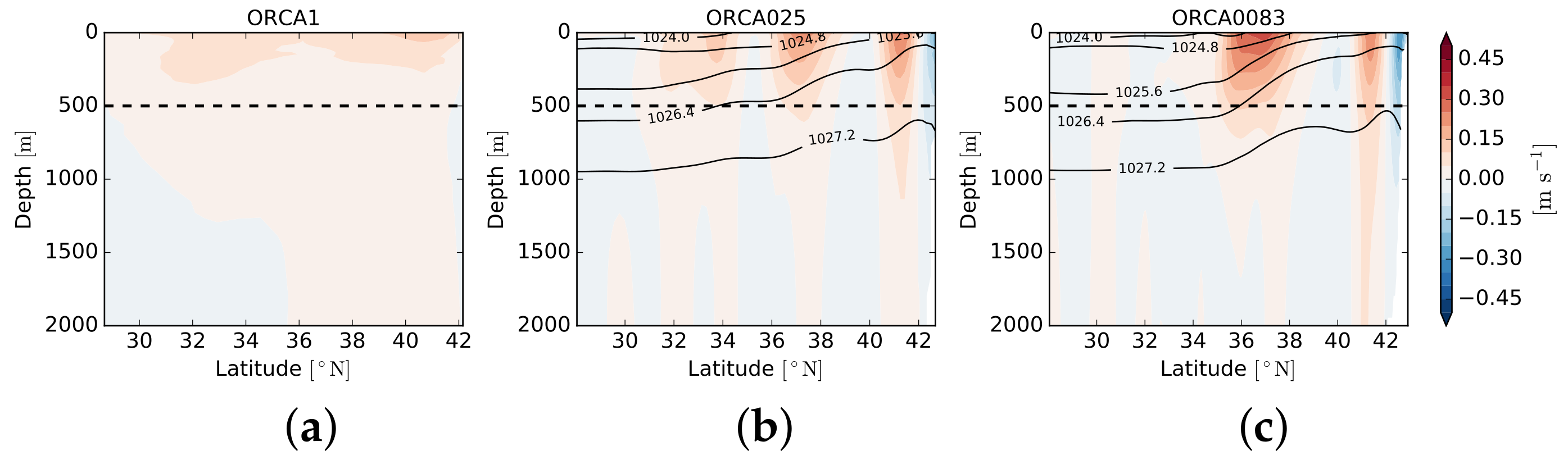
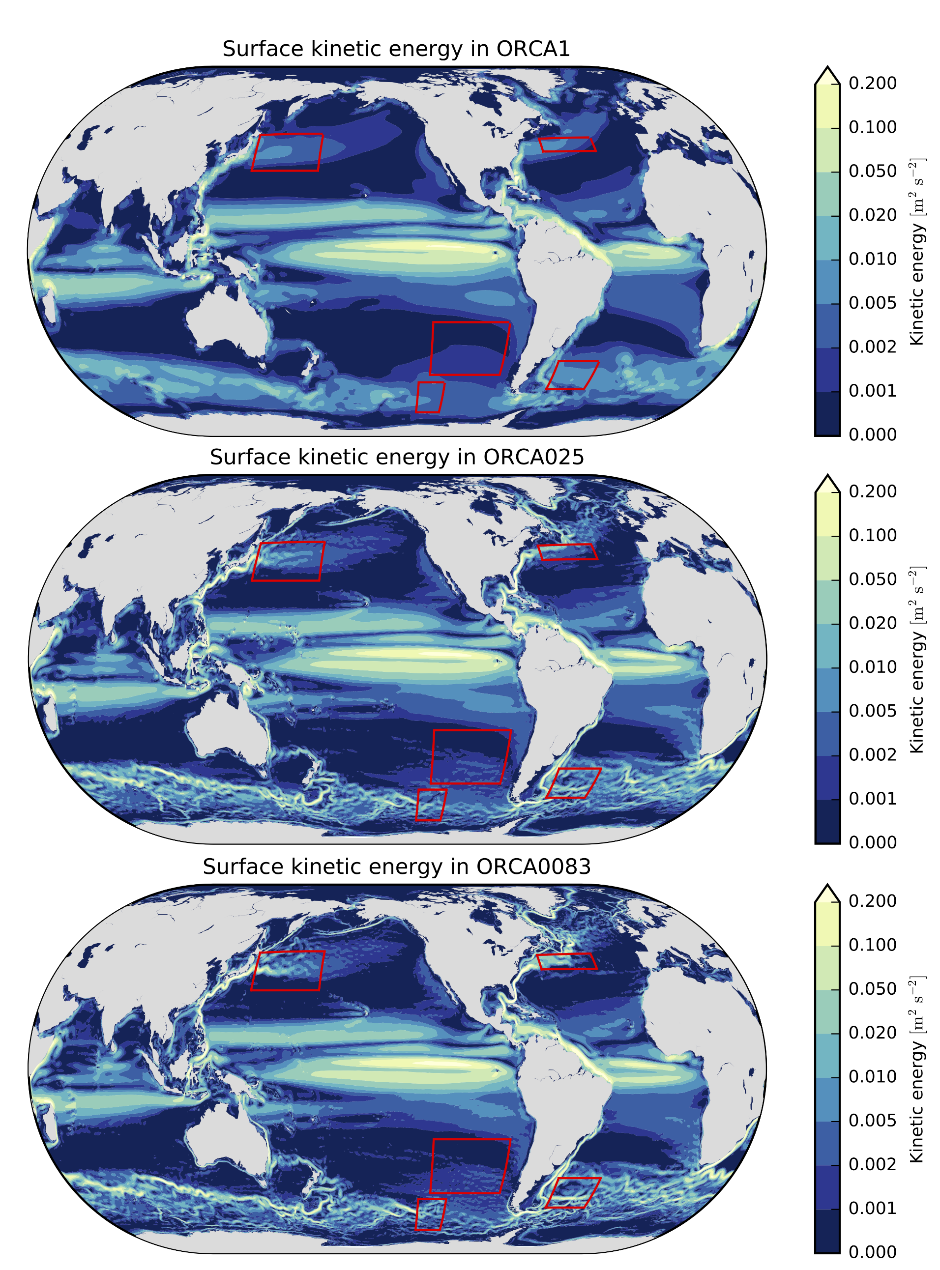
In regions of strong currents and eddy activity such as the Kuroshio, ACC and the Gulf Stream, the eddy-resolving ORCA0083 simulation has higher surface KE than the lower-resolution simulations (Figure 2). For individual snapshots (not shown), ORCA0083 also has a clear eastward extension of both the Kuroshio and Gulf Stream which is not simulated in ORCA025 or ORCA1. Such an extension can also be seen in observations from satellite altimetry (not shown). A more energetic upper ocean is also found when looking at a latitude–vertical cross section of the Kuroshio current along (Figure 1), where the jet has a peak zonal velocity of in ORCA0083, in ORCA025 and in ORCA1. Similar differences are found for the Gulf Stream, ACC and the Malvinas. The zonal velocity is higher and the horizontal density gradients are sharper in ORCA0083 than in ORCA025 and ORCA1, partly because higher-resolution models can resolve sharper gradients, but also because there is less horizontal viscosity and diffusivity that smooths horizontal velocity and density gradients.
We average the model data onto two levels, upper ocean (level 1) and deep ocean (level 2), separated at in the Kuroshio region as described in Section 3. As also mentioned in Section 3, we have experimented with different values of and found that, while the absolute values of our calculations can change, the main results remain valid. The separation between the upper and deep ocean is shown in Figure 3 to approximately separate high KE, strong stratification, and clear seasonal variability in the upper ocean from low KE, weak stratification and very little variability at depth. We calculate root-mean-square vertical shear and upper-ocean density anomalies as
where subscripts indicate the upper and lower layers, is an area average and is a time average over 1979-2009. We find that the mean vertical shear, as well as the density anomalies in the upper layer, are greater in ORCA0083 than in the two other simulations in all regions (Kuroshio shown in Figure 4). The ORCA0083 simulation has larger density anomalies in the upper ocean Kuroshio, which indicates more buoyancy in the upper layer, , and thus more available potential energy (APE) in ORCA0083 than ORCA025 and ORCA1, since [40]. The ORCA025 and ORCA0083 simulations have relatively similar profiles of , while ORCA1 is different (Figure 3), and this is generally true for all regions studied here. Calculating APE as [40], we find more APE in ORCA0083 than ORCA025 and ORCA1 in the Kuroshio as well as the other regions marked in Figure 2. Hence, even though the surface buoyancy forcing is the same in the three simulations, there is more APE that may be converted to KE in ORCA0083.
All three simulations have a strong annual cycle in upper-ocean density anomalies, , likely due to the annual cycle in solar heating and freshwater forcing (Figure 4b,d). The power spectrum of shows a stronger semi-annual cycle in ORCA1 than ORCA025 and ORCA0083, which can also be seen in the timeseries. All simulations also have a pronounced annual cycle in mean vertical shear of velocity, , (Figure 4a,c) caused mostly by an annual cycle in winds that changes upper-ocean KE (Figure 3), although it is progressively weaker with lower horizontal resolution. We also find low-frequency variability that is stronger or as strong as annual variability in all simulations and all regions. We stress that all three simulations are forced with the same wind and buoyancy forcing and have the same vertical resolution. The low-frequency variability that impacts the Kuroshio may be the Pacific Decadal Oscillation (PDO) [41]. Low-frequency variability has also been reported in observations of the Gulf Stream [42], and ocean-only modelling experiments of the ACC [43], which may explain the high spectral power at long time scales for these regions (not shown). The ORCA1 simulation generally has an order of magnitude weaker variability on timescales longer than one month. We also find ORCA025 to have a less distinct annual cycle in the timeseries of (Figure 4a), due to the fact that annual variability has less spectral power than low-frequency variability in that simulation. However, in ORCA0083, the annual and inter-annual variabilities are of similar power and the annual cycle is more distinct in the timeseries. The differences between the three simulations in annual and low-frequency variability is likely due to the fact that the temporal inverse cascade of KE, i.e., the transfer of KE from monthly to inter-annual timescales, is weaker with lower resolution [44,45].
4.2. Spectral Fluxes in the Upper Ocean
We are interested in the impact of horizontal resolution on the KE balance of oceanic flows and will therefore focus on the KE in four regions of high eddy activity and one region with low eddy activity. The five regions are marked in Figure 2: the ACC in the Pacific sector, the Malvinas region in the South Atlantic, the Kuroshio extension, the Gulf Stream extension and, for comparison, a region in the East Pacific where eddy activity is low. The ACC region is the same as studied by [10], which allows for a comparison with their results. We will use only the upper ocean, defined in Section 3, and investigate the Fourier transformed KE budget defined in Equation (6).
We calculate the spectral KE density, , from Equation (5) for all regions (Figure 5). We find that the eddy-resolving ORCA0083 simulation has more KE than the other two simulations at all wavenumbers. We also find that the energy-containing scale is shifted from ∼320 to ∼280 from ORCA025 to ORCA0083 in the Kuroshio, and observe similar shifts for the other regions. However, if the energy-containing scale is defined by the peak in , as in [15,46], then we find no change in the energy-containing scale between ORCA025 and ORCA0083. The non-eddying ORCA1 run has at least an order of magnitude less KE than the other two simulations, which is true whether the eddy-induced velocities from the GM scheme are added to the Eulerian velocities or not. We also find that ORCA025 and ORCA0083 have a clear peak near the scale, while ORCA1 has no peak. Hence, the KE spectra in ORCA025 and ORCA0083 peak near their respective energy-containing scales. As we will show later in this section, KE fluxes converge to the energy-containing scale of ∼200–300 in all regions of eddy activity studied here. The KE spectra (Figure 5) are somewhat steeper than the slope predicted in the 2D turbulence inertial range when stirring and dissipation are isolated to large and smaller scales respectively. The slope is steeper for ORCA025 than ORCA0083. As we will show later, the spectral fluxes due to wind forcing and PE to KE conversion occur over a range of wavenumbers, and thus there is no clear inertial range where a slope could be expected.
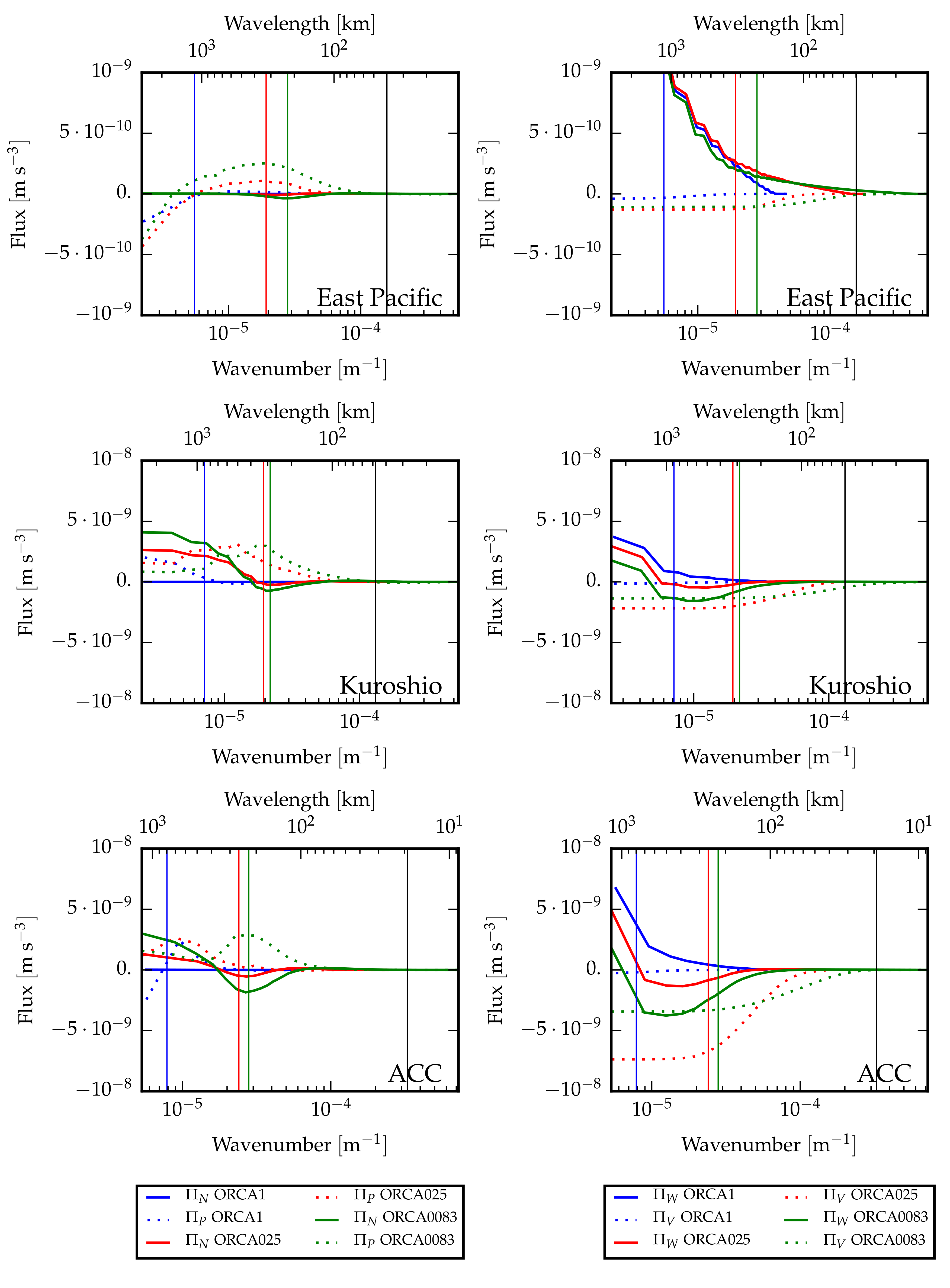
The two eddying configurations, ORCA025 and ORCA0083, clearly show negative spectral fluxes for nonlinear interactions, , corresponding to KE transfer from smaller to larger scales, i.e., an inverse cascade, with a peak near the energy-containing scale of ∼300 (Figure 6). An inverse cascade corresponds to either eddies merging into larger eddies, or eddies rectifying a jet such as the Kuroshio, as found in previous results for global ocean models, e.g., [1,27]. We find positive values of with a peak near the energy-containing scale, hence opposite the inverse cascade of KE (Figure 6).
The scale at which and peak is larger than the Rossby radius of deformation, , shown in Figure 5 for ORCA0083.
However, the fastest growing mode can be up to a factor larger than the Rossby radius wavelength, [19,33]. Taking , which is the average Rossby radius in our ACC region, gives which is close to the peak of the inverse cascade, , and PE to KE conversion, . The positive lobe of PE to KE conversion corresponds to adding KE to scales smaller than the energy-containing scale and removing KE from the larger scales.
The energy-containing scale of ∼300 is significantly larger than the first baroclinic Rossby radius (Figure 6), and larger than the horizontal resolution of ORCA1. However, since ORCA1 does not resolve or parameterise the process by which KE fluxes to larger scales, the high KE at the energy-containing scale can not be simulated by ORCA1.
The inverse cascade of KE, , is stronger in ORCA0083, weaker in ORCA025, and nearly zero in ORCA1 in all regions, which is in agreement with [1,20] who found that increasing viscosity or using coarser horizontal resolution in an idealised model dissipates KE that would otherwise be transferred to larger scales. Here, it is confirmed to also be the case in state-of-the-art global ocean models with realistic bathymetry and forcing. Similarly to the inverse cascade, and in agreement with [47], the conversion of PE to KE, , attain larger values in ORCA0083, than in ORCA025 or ORCA1. More conversion of PE to KE in ORCA0083 than ORCA025 and ORCA1 implies stronger horizontal pressure gradients and thus a stronger geostrophic flow, which can be seen in a cross section of the Kuroshio (Figure 1) and the other regions studied (not shown), where the zonal flow and the meridional density gradients are stronger at higher resolution. As previously noted, stronger horizontal pressure gradients can be explained by the higher horizontal resolution as well as the lower iso-neutral tracer diffusion. In combination, this means that, in ORCA025, buoyancy anomalies will be subjected to more tracer diffusion and at somewhat larger scales than in ORCA0083. Hence, even though all three simulations have the same surface buoyancy forcing, higher horizontal resolution makes the ocean model more efficient in converting PE to KE.
We find that the spectral transfer for wind forcing, , is the same at scales , i.e., has the same slope, for all three simulations, but they differ near the energy-containing eddy scales. Wind forcing is a source of energy at larger scales but, for ORCA025 and ORCA0083, wind forcing is also a sink of KE at near the energy-containing scale. This is due to the fact that zonal wind stress accelerates a zonal jet, but induces a torque that opposes the vorticity of the eddies so that eddies lose KE [48]. Eddies on scales near the energy-containing scale in ORCA0083 lose KE to wind forcing and viscosity in roughly equal portions, while, in ORCA025, viscosity dominates over wind (Figure 6). Hence, the manner by which eddies lose KE can be very different depending on the horizontal resolution of the model. It is not clear if this impacts the shape or the lifespan of eddies. Overall, the net KE input from wind is largest in ORCA1 for all regions, except in the East Pacific where there is almost no eddy activity and thus the wind forcing is identical in all three simulations. We note that the KE budgets in Figure 6 do not close perfectly. As stated in Section 3, vertical viscosity and vertical momentum transfer are omitted due to being small but still introduce small errors when attempting to close the budget. However the largest errors in the budget are due to interpolation errors and fluxes of KE on the lateral boundaries of the regions studied. In all simulations, there is a non-zero flux of KE in and out of all the regions studied. We have repeated our calculations using the output of an idealised double-gyre simulation with settings similar to ORCA025, and found that the spectral fluxes sum to nearly zero on the boundaries.
In geostrophic turbulence, the inverse cascade is predicted to terminate near the Rhines scale where most of the KE is contained within large-scale Rossby waves. The Rhines scale is defined as [49], where is the root-mean-square zonal velocity and . The Rhines scale scales with the eddy KE, and is thus smaller in ORCA025 than in ORCA0083, implying that the inverse cascade can act over a wider range of scales in ORCA0083 than in ORCA025. The Rhines scale has also been found to coincide with the peak of the KE spectrum [49,50], i.e., the peak of the KE spectrum shifts toward smaller scales at lower resolution [19] However, we find neither a shift in the peak of the KE spectrum (Figure 5) nor a shift in the scale at which the inverse cascade arrests (Figure 6) from ORCA025 to ORCA0083 in any of the regions studied. We note that the change in Rhines scale from ORCA025 to ORCA0083 in all regions is only ∼5–10 , which is too small to be resolved in the simulations. Therefore while the eddy resolving model has more eddy KE than the eddy permitting simulation, this change in eddy KE is not large enough to drastically impact the Rhines scale or the arrest of the inverse cascade. This explains why the peak of the KE spectrum and the inverse cascade do not shift from ORCA025 to ORCA0083. We find two orders of magnitude difference in KE between ORCA1 and ORCA025, and thus a much larger difference in Rhines scale between ORCA1 and ORCA025 than between ORCA025 and ORCA0083. However, ORCA1 has no clear peak of the KE spectrum and no inverse cascade, so we can not relate the change in Rhines scale between ORCA1 and ORCA025 to a shift in scale where the inverse cascade arrests.
The non-eddying simulation, ORCA1, generally shows almost no spectral flux from nonlinear interactions or PE to KE conversion except at the largest scales. We include the eddy-induced velocities in our analysis, which are responsible for some conversion of PE to KE by flattening isopycnals to generate eddy velocities. This could be the positive seen at large scales in ORCA1 (Figure 6). It is clear, however, that the eddy-induced velocities do not result in an inverse KE cascade, which may be the main reason for the low KE.
4.3. Baroclinic and Barotropic Kinetic Energy (KE)
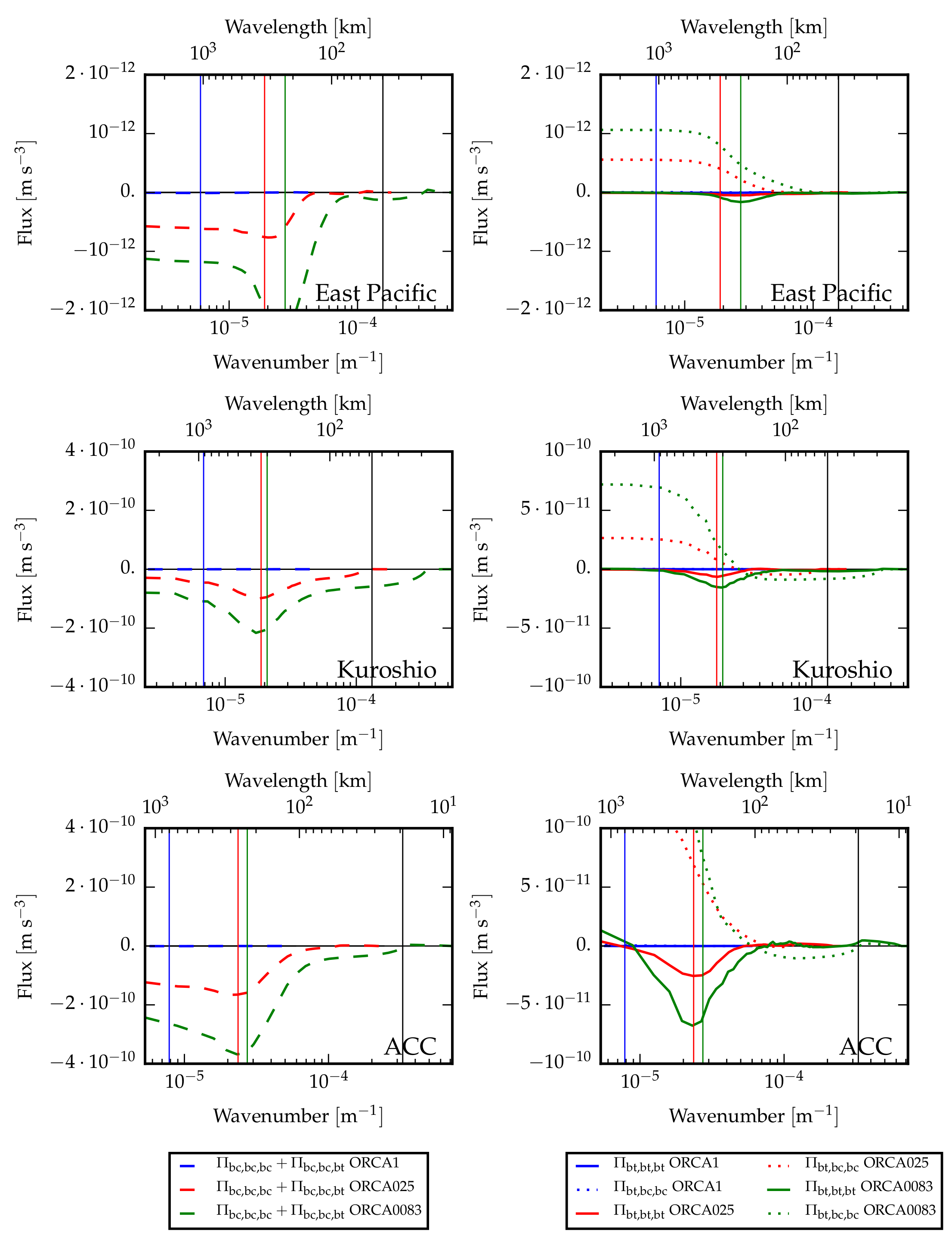
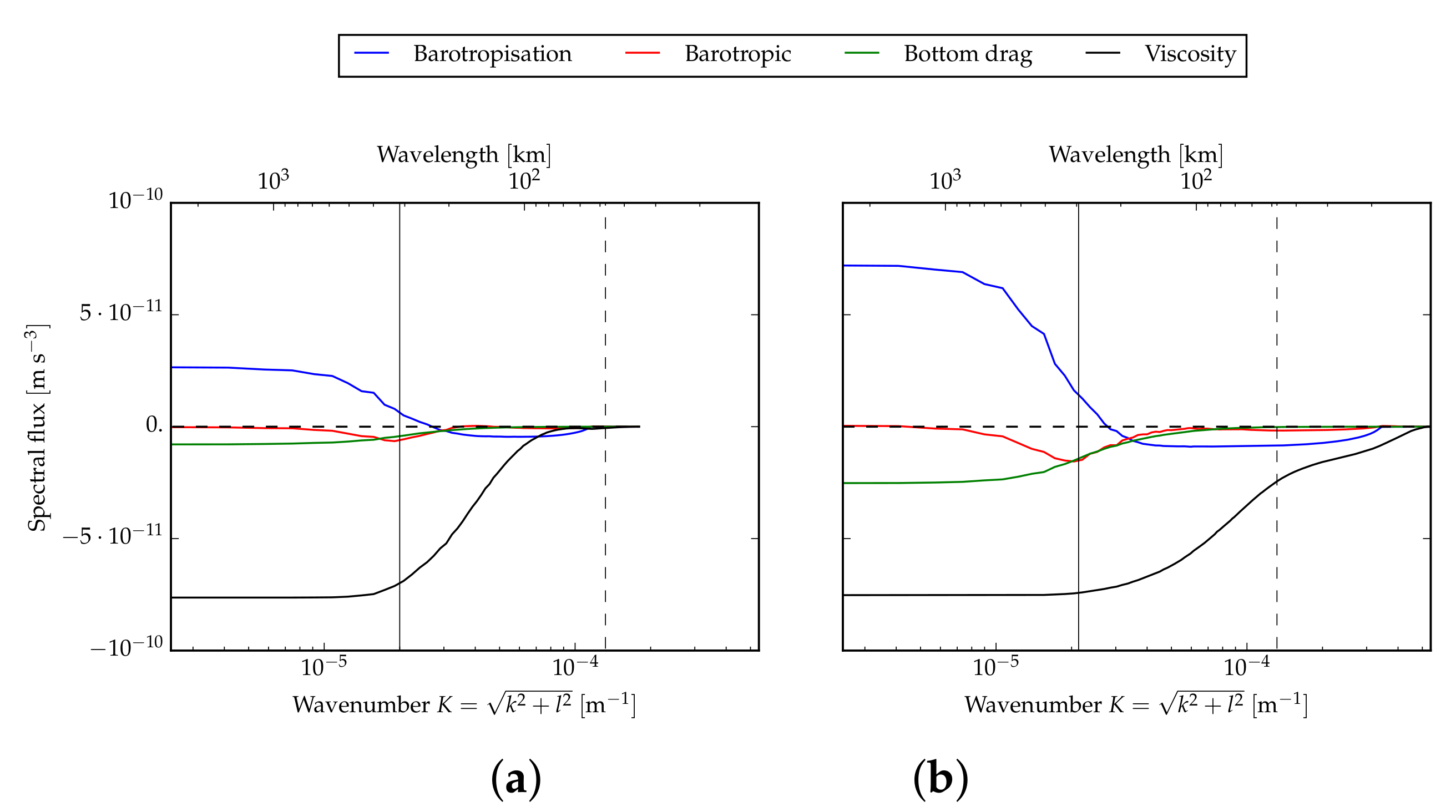
As described in Section 3, we average the model data onto two vertical layers, representing the upper and deep ocean, to limit the effect of bathymetry. We calculate the barotropic spectral flux, , the baroclinic spectral flux (with the added catalytic flux), , and the spectral flux due to barotropisation, [16] as described in Appendix A. We find a distinct inverse cascade in both the barotropic and baroclinic modes (Figure 7), similar to [16], in all regions, although it is very weak in the East Pacific. The two terms and have very similar structure, thus adding the catalytic flux to the baroclinic self-interaction enchances the total baroclinic KE flux. In both ORCA025 and ORCA0083, barotropisation injects KE over the 150–600 range, and the barotropic inverse cascade transfers energy from the 150–300 range to the 300–600 range (Figure 8). This implies a KE sink over this range, which can partly be explained by bottom drag (Figure 8), and wind forcing (Figure 6). The scales over which barotropisation acts, as well as the scale at which the barotropic KE spectrum peaks, are unchanged from ORCA025 to ORCA0083. It is difficult to conclude whether the abovementioned scales are insensitive to horizontal resolution from studying just two eddying simulations.
The baroclinic inverse cascade does not approach zero at the smallest wavenumber, implying that the energy-containing scales drive baroclinic flow on scales larger than the regions studied here. The results show that the baroclinic inverse cascade is about ∼7–10 times larger than barotropic inverse cascade in both ORCA025 and ORCA0083. This is likely due to the strong bottom friction [51] which, in idealised models, results in a baroclinic inverse cascade much larger than the barotropic inverse cascade [16]. Furthermore, we find that the East Pacific region has inverse cascades of barotropic and baroclinic KE, but of at least one order of magnitude smaller than in the other regions due to the low eddy activity. As is the case for the KE cascades in the upper ocean, the ORCA025 simulation clearly has weaker inverse cascades of barotropic and baroclinic KE than ORCA0083. It is clear that the ORCA1 simulation has virtually no KE cascades, as shown for the upper ocean (Figure 6). We stress that with our two-layer approach, all baroclinic modes are encapsulated into one. The inverse cascade of baroclinic KE may thus be a residual of an inverse cascade in the first baroclinic mode and forward cascades in the higher modes [10,11], and the partitioning of KE between baroclinic modes can differ between simulations. For realistic ocean stratifications, KE is efficiently transferred from higher baroclinic modes to the first baroclinic mode, and subsequently to the barotropic mode [13,52]. It is therefore likely that the barotropisation mostly represents the transfer between the first baroclinic mode and the barotropic mode.
We find clear differences in the strength of barotropisation between our simulations, with stronger barotropisation in ORCA0083 than ORCA025 and very small barotropisation in ORCA1. The differences in barotropisation could be due to differences in bottom friction, stratification, or barotropic eddy KE, which have been show to impact the barotropisation [11,12,13,14,15,16,46]. Comparing ORCA025 to ORCA0083 in each region, we find that the mean stratification, , in the upper ocean (Figure 3) is similar in both simulations, and can thus not explain the differences in barotropisation between the simulations. Differences in bottom drag in the barotropic mode (shown for the Kuroshio in Figure 8), can explain some of the stronger barotropisation at higher resolution [15]. Furthermore, some of the differences in barotropisation can also be explained by the fact that horizontal viscosity dominates over barotropisation and the barotropic inverse cascade in ORCA025, but not in ORCA0083. While the relative effects of bottom drag and horizontal viscosity on the barotropisation are unclear from our results, we note that [15] found bottom drag to have a low effect on barotropisation. Hence, we speculate that horizontal viscosity is the dominant factor here. To isolate the impact of bottom drag, one could run multiple ORCA025 and ORCA0083 simulations with varying bottom drag coefficient, , but this is beyond the scope of this paper.
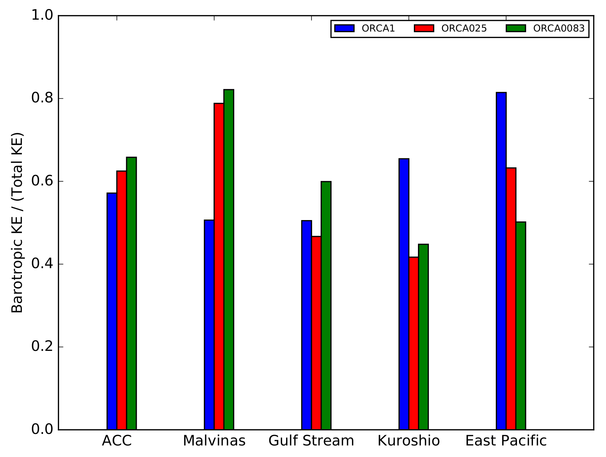
For each of the regions, we calculate the area-averaged barotropic and baroclinic KE, and then the fraction of the total KE that is in the barotropic mode (Figure 9). For the western boundary currents, the ORCA0083 simulation agrees with observations [38], where it was reported that the Kuroshio and Gulf Stream have about and of the total KE in the barotropic mode, respectively. We find that the ACC and Malvinas have ∼60% and ∼80% of KE in the barotropic mode, respectively, but it is difficult to compare to observations as there is very poor observational coverage for these regions in [38], and we are unaware of any other observations of this. We find that in all regions except the East Pacific, the flow is more barotropic in ORCA0083 than in ORCA025. The weaker barotropisation in ORCA025 compared to ORCA0083 (Figure 7) suggests that the lack of barotropic energy in ORCA025 is due to less barotropisation, which can be explained by baroclinic eddies that are becoming more barotropic being dissipated faster in ORCA025. In the ACC, Malvinas and Gulf Stream, the ORCA1 simulation is even less barotropic than the other simulations, while, in the Kuroshio, it is strongly barotropic. Thus, horizontal resolution can have an impact on the vertical structure of the simulated flow by changing the partition of barotropic and baroclinic KE, which can be seen as a bias in e.g., the vertical shear.
5. Discussion and Conclusions
We have presented the energy budget for state-of-the-art global ocean simulations of varying resolution, which allowed us to study the impact of horizontal resolution on the flow in models with realistic bathymetry, wind forcing, and bottom drag. To our knowledge, a spectral KE budget for state-of-the-art ocean models has not been presented before. The eddy-permitting simulation, ORCA025, showed a weaker inverse cascade of KE than the eddy-resolving simulation, ORCA0083 (Figure 6), which was caused partly by the lower horizontal resolution, and partly by the necessary higher viscosity. There were also clear differences in the effect of wind forcing and conversion of PE to KE between ORCA025 and ORCA0083 (Figure 6). As a result, in ORCA025 currents were too weak (Figure 1), the midlatitude jets did not extend far enough eastward (Figure 2), and viscosity had a dominating effect on the KE budget.
We found no shift in the scale at which the KE spectrum peaks from ORCA025 to ORCA0083, and also that the inverse cascade acted over the same range of scales in both simulations. However, in idealised experiments, Jansen, et al. [19] found that the peak of the KE spectrum shifts to larger scales with higher resolution, which implies that the inverse cascade arrests at larger scales as well. We explain this disagreement by the fact that the Rhines scale, which predicts where the inverse cascade arrests and the KE spectrum peaks, changed by only ∼5–10 from ORCA025 to ORCA0083. Hence, the shift in Rhines scale was too small to be resolved by either the ORCA025 or the ORCA0083 simulations. The small differences in the Rhines stem from the small differences in eddy KE between the eddy permitting and eddy resolving simulations. We similarly found no shift in the scales over which the barotropisation and the barotropic inverse cascade act from ORCA025 to ORCA0083. Studying how these macroturbulent scales change with horizontal resolution is interesting and would require a larger suite of eddying simulations than the two (ORCA025 and ORCA0083) presented here.
Several studies [12,13,15] have investigated the sensitivity of barotropisation to e.g., stratification, bottom drag and Coriolis parameter. However, to our knowledge, none of these studies investigated the sensitivity of barotropisation to horizontal resolution or horizontal viscosity. We found that differences in stratification, (Figure 3), could not explain the large differences in barotropisation. Comparing ORCA025 to ORCA0083, we found that the stronger bottom drag at higher resolution could explain at least part of the stronger barotropisation, although bottom drag was noted to have a low effect on barotropisation in [15]. The differences in horizontal viscosity and resolution may explain some of the differences in barotropisation as well, as horizontal viscosity has a much larger impact on the barotropic KE budget in ORCA025 than in ORCA0083 (Figure 8). Further sensitivity studies are needed to fully understand the impact of viscosity and bottom drag on barotropisation in realistic global ocean models.
Partitioning the KE into barotropic and a baroclinic mode, we found that the ORCA025 simulation had a more baroclinic flow than ORCA0083, since part of the KE that should be transfered from the baroclinic mode to the barotropic mode is dissipated by the higher viscosity, although bottom drag was lower. This suggests that increasing the horizontal resolution or reducing horizontal viscosity (while maintaining numerical stability) can reduce biases in the simulated vertical structure, although the vertical resolution is important as well. When the flow is too baroclinic, it will impact the relative importance of terms such as buoyancy forcing over Reynolds stresses in the eddy energy budget. Bottom drag, which primarily affects the barotropic mode [16] and is the primary way of dissipation in the ocean [51], was underestimated in ORCA025 due to the lower barotropic KE, thus changing the relative importance of drag and viscosity on KE dissipation. Furthermore, the vertical structure of the flow, to some extent, set the level at which the effective horizontal mixing is largest in regions like the ACC or western boundary currents [53,54,55]. Thus, simulating a realistic vertical structure is of vital importance for the horizontal mixing of tracers in the model.
Our findings show that the some key processes in mesoscale eddies can be different in eddy-resolving and eddy-permitting ocean models. The eddy-resolving ORCA0083 had a significantly larger sink of oceanic eddy KE due to wind forcing than the eddy-permitting ORCA025. An eddy KE sink implies a transfer of momentum from the ocean to the atmosphere, which in turn implies that, as horizontal resolution of the ocean in coupled climate models increases, the momentum budget for the atmospheric boundary layer will change. The shapes of eddies may also be different, as high viscosity could prevent eddies from becoming horizontally anisotropic [56] and the lack of barotropisation leads to too much vertical shear.
For ORCA025 and ORCA0083, our spectral KE budget results agree with the energy cycle in physical space diagnosed by [57] who showed a route of energy where mean KE and mean PE can generate eddy PE, which is then converted to baroclinic eddy KE and lastly barotropic eddy KE. This is also mostly in line with [58]. In the Lorenz energy cycle by [58], winds and dissipation are the main source and sink for eddy KE, respectively. However, our results show that conversion from eddy PE is the main source of eddy KE, while both dissipation and winds act as sinks, similarly to [48,59]. In the framework of a Lorenz energy cycle, our results show that all parts of the transfer from mean PE to eddy PE and subsequently to eddy KE are weaker at eddy-permitting resolution and that their underestimation is balanced by higher rates of dissipation of KE and diffusion of PE.
We suggest that we can improve the eddy-permitting simulation by decreasing viscosity, parameterising PE to KE conversion or parameterising sub-grid transfers of KE. Lowering the horizontal viscosity parameter, , can lead to some improvements of the simulated currents but also leads to more numerical noise [60]. A more promising way to improve the simulations is to use a flow-dependent viscosity [21,22] where the dissipation is set by the deformation rate or vorticity gradients. Such methods generally lead to improvements by having overall less dissipation while still suppressing numerical noise [23,61], which could result in a stronger inverse cascade of KE and more barotropisation.
It is possible to improve eddy-permitting simulations by amplifying the PE to KE conversion, i.e., strengthening the horizontal pressure gradients (Figure 6). Such an approach was taken by [26], who used stochastic processes to represent unresolved density fluctuations in a coarse-resolution model. Brankart, et al. [26] found that the parameterisation resulted in more ageostrophic motions, more intense vertical velocities, and improvements in many regions with intense eddy activity. Using a coupled climate model, Ref. [62] found that the parameterisation by [26] reduced some of the biases in low-resolution climate models as well as increased the interannual variability of the overturning circulation. Horizontal pressure gradients can also be strengthened by strengthening horizontal gradients of sea surface height, which would require increasing the divergence of the barotropic velocities, e.g., using a stochastic parameterisation to represent unresolved divergent motions.
Despite the fact that the KE input from wind forcing at large scales was very similar in all simulations, the ORCA0083 simulation had more KE at all wavenumbers due to a stronger inverse cascade (Figure 5). A way to improve eddy-permitting simulations like ORCA025 is to parameterise or enhance the inverse cascade of KE, which can be done in a few different ways. The “backscattering” parameterisation by [19] aims to calculate the KE lost due to viscosity and re-inject it at larger scales in order to parameterise the inverse cascade. The “ model” by [63,64] uses filtered velocities where Rossby radius is shifted to larger scales, thus making it more clearly resolved. Work has also been done using the “Rivlin–Ericksen” stress [20,25] where subgrid eddy stresses are represented by a stress tensor that can strengthen velocity gradients and thus amplify eddies. Implementing the above parameterisations in ocean models [20,64,65] has shown that they enhance the inverse cascade and allow an eddy-permitting model to have a KE spectrum more similar to that of an eddy-resolving model.
Future work should involve calculating KE budgets for ocean models of even higher horizontal resolution that include sub-mesoscales and internal waves, e.g., -MITgcm simulation [66], to diagnose to what extent the ORCA0083 simulation underestimates KE of ocean currents and eddies. We would also propose to perform sensitivity experiments with state-of-the-art global ocean models to disentangle the roles of horizontal resolution, bottom drag and horizontal viscosity in controlling barotropisation. This would help in understanding what sets the scales of the inverse cascade and the peak of the KE spectra in our simulations, which could be studied using a larger suite of simulations of varying horizontal resolution. In the future, we also hope to investigate the KE budgets in global ocean models that utilise some of the parameterisations mentioned above, e.g., scale-aware viscosity or augmented energy transfers, to see how well they may reduce biases in the inverse cascade of KE or barotropisation for eddy-permitting models. Work is currently ongoing to implement and test new parameterisations of subgrid energy transfers for state-of-the-art ocean models.
Acknowledgments
We sincerely thank Rei Chemke and two anonymous reviewers, whose comments improved the paper greatly. We thank Andrew Coward for performing the NEMO simulations and giving us access to the output. We thank Thomas Bolton and Tomos David for useful discussions and suggestions. All numerical calculations where performed on the Jasmin storage and computing centre provided by the Centre for Environmental Data Analysis (CEDA). Funding is by Natural Environment Research Council (NERC) grants No.NE/K013548/1 and grants No.NE/J00586X/1.
Author Contributions
Joakim Kjellsson and Laure Zanna designed the research. Joakim Kjellsson performed the analysis of the data. Joakim Kjellsson and Laure Zanna wrote the paper.
Conflicts of Interest
The authors declare no conflict of interest.
Appendix A
We decompose the KE budget (Equation (1)) into barotropic and baroclinic components by inserting into the momentum equations from NEMO [28]. Then, multiplying by the barotropic velocities, , we find the contributions to the barotropic KE budget as
where vertical nonlinear interactions and vertical viscosity are ignored as there is no vertical component in the barotropic mode. We multiply by baroclinic velocities, , in the upper and lower layers and integrate vertically to get the baroclinic KE budget as
As in the main text, is a vertical average over the two layers and . Re-arranging the nonlinear interactions gives, for the barotropic KE budget,
We note that terms including only one baroclinic component integrate to zero vertically. The first remaining term, , is the barotropic self-interaction since it involves only the barotropic mode; The second, , is the barotropisation, which is a transfer of KE from the baroclinic mode to the barotropic mode. The nonlinear interactions in the baroclinic KE budget are
The first remaining nonlinear interaction in the baroclinic KE budget is “barotropic stirring”, , which represents baroclinic energy advected by the barotropic mode and corresponds to the barotropisation in the barotropic KE budget [16]. The second term is the “catalytic” term [16], , which involves the barotropic mode and redistributes KE within the baroclinic mode. The last term involves only the baroclinic mode and is the baroclinic self-interaction, . The barotropic and baroclinic KE budgets are thus
where the barotropic forcing, , includes the surface pressure gradient term and wind forcing, while barotropic dissipation, , includes bottom drag and horizontal viscosity from Equation (A1). Baroclinic forcing, , includes the hydrostatic pressure gradient term, wind forcing and vertical momentum transfer, while dissipation, , includes bottom drag, horizontal viscosity and vertical viscosity from Equation (A2). Following [16], we add the baroclinic self-interaction to the “catalytic” term to get the total baroclinic nonlinear interactions, . We find that both are very similar in sign and magnitude. In our calculations, barotropic stirring is the smallest term in the baroclinic KE budget, and we therefore ignore it.
In spectral space, the barotropic and baroclinic KE budgets are found in the same way as the full KE budget (Equation (6)):
where, as before, a spectral flux, , is found by integrating the spectral transfer, , over wavenumbers. The spectral transfers for the KE budget are
where, as in the main text, curly braces {} denote Fourier transformed variables, and square brackets, denotes a vertical average.
References
- Arbic, B.K.; Polzin, K.L.; Scott, R.B.; Richman, J.G.; Shriver, J.F. On eddy viscosity, energy cascades, and the horizontal resolution of gridded satellite altimeter products. J. Phys. Oceanogr. 2012. [Google Scholar] [CrossRef]
- Hallberg, R.W. Using a resolution function to regulate parameterizations of oceanic mesoscale eddy effects. Ocean Model. 2013, 72, 92–103. [Google Scholar] [CrossRef]
- Hewitt, H.T.; Roberts, M.J.; Hyder, P.; Graham, T.; Rae, J.; Belcher, S.E.; Bourdallé-Badie, R.; Copsey, D.; Coward, A.; Guiavarch, C.; et al. The impact of resolving the Rossby radius at mid-latitudes in the ocean: Results from a high-resolution version of the Met Office GC2 coupled model. Geosci. Model Dev. 2016, 9, 3655–3670. [Google Scholar] [CrossRef]
- Zhang, Y.; Vallis, G.K. Ocean Heat Uptake in Eddying and Non-Eddying Ocean Circulation Models in a Warming Climate. J. Phys. Oceanogr. 2013, 43, 2211–2229. [Google Scholar] [CrossRef]
- Oschlies, A. Improved Representation of Upper-Ocean Dynamics and Mixed Layer Depths in a Model of the North Atlantic on Switching from Eddy-Permitting to Eddy-Resolving Grid Resolution. J. Phys. Oceanogr. 2002, 32, 2277–2298. [Google Scholar] [CrossRef]
- Griffies, S.M.; Winton, M.; Anderson, W.G.; Benson, R.; Delworth, T.L.; Dufour, C.O.; Dunne, J.P.; Goddard, P.; Morrison, A.K.; Rosati, A.; et al. Impacts on Ocean Heat from Transient Mesoscale Eddies in a Hierarchy of Climate Models. J. Clim. 2015, 28, 952–977. [Google Scholar] [CrossRef]
- Kraichnan, R.H. Inertial Ranges in Two-Dimensional Turbulence. Phys. Fluids 1967, 10, 1417–1423. [Google Scholar] [CrossRef]
- Kolmogorov, A.N. Dissipation of Energy in the Locally Isotropic Turbulence. Proc. Math. Phys. Sci. 1991, 434, 15–17. [Google Scholar] [CrossRef]
- Salmon, R. Baroclinic instability and geostrophic turbulence. Geophys. Astrophys. Fluid Dyn. 1980, 15, 167–211. [Google Scholar] [CrossRef]
- Scott, R.B.; Wang, F. Direct Evidence of an Oceanic Inverse Kinetic Energy Cascade from Satellite Altimetry. J. Phys. Oceanogr. 2005, 35, 1650–1666. [Google Scholar] [CrossRef]
- Fu, L.L.; Flierl, G.R. Nonlinear energy and enstrophy transfers in a realistically stratified ocean. Dyn. Atmos. Oceans 1980, 4, 219–246. [Google Scholar] [CrossRef]
- Held, I.M.; Larichev, V.D. A Scaling Theory for Horizontally Homogeneous, Baroclinically Unstable Flow on a Beta Plane. J. Atmos. Sci. 1996, 53, 946–952. [Google Scholar] [CrossRef]
- Smith, K.S.; Vallis, G.K. The Scales and Equilibration of Midocean Eddies: Freely Evolving Flow. J. Phys. Oceanogr. 2001, 31, 554–571. [Google Scholar] [CrossRef]
- Treguier, A.M.; Hua, B.L. Influence of bottom topography on stratified quasi-geostrophic turbulence in the ocean. Geophys. Astrophys. Fluid Dyn. 1988, 43, 265–305. [Google Scholar] [CrossRef]
- Chemke, R.; Kaspi, Y. The latitudinal dependence of the oceanic barotropic eddy kinetic energy and macroturbulence energy transport. Geophys. Res. Lett. 2016, 43, 2723–2731. [Google Scholar] [CrossRef]
- Scott, R.B.; Arbic, B.K. Spectral Energy Fluxes in Geostrophic Turbulence: Implications for Ocean Energetics. J. Phys. Oceanogr. 2007, 37, 673–688. [Google Scholar] [CrossRef]
- Capet, X.; McWilliams, J.C.; Molemaker, M.J.; Shchepetkin, A.F. Mesoscale to Submesoscale Transition in the California Current System. Part III: Energy Balance and Flux. J. Phys. Oceanogr. 2008, 38, 2256–2269. [Google Scholar] [CrossRef]
- Gent, P.R.; McWilliams, J.C. Isopycnal mixing in ocean circulation models. J. Phys. Oceanogr. 1990, 20, 150–155. [Google Scholar] [CrossRef]
- Jansen, M.F.; Held, I.M. Parameterizing subgrid-scale eddy effects using energetically consistent backscatter. Ocean Model. 2014, 80, 36–48. [Google Scholar] [CrossRef]
- Zanna, L.; Porta Mana, P.; Anstey, J.; David, T.; Bolton, T. Scale-aware deterministic and stochastic parametrizations of eddy-mean flow interaction. Ocean Model. 2017, 111, 66–80. [Google Scholar] [CrossRef]
- Griffies, S.M.; Hallberg, R.W. Biharmonic Friction with a Smagorinsky-Like Viscosity for Use in Large-Scale Eddy-Permitting Ocean Models. Mon. Weather Rev. 2000, 128, 2935–2946. [Google Scholar] [CrossRef]
- Fox-Kemper, B.; Menemenlis, D. Can Large Eddy Simulation Techniques Improve Mesoscale Rich Ocean Models? In Ocean Modeling in an Eddying Regime; American Geophysical Union: Washington, DC, USA, 2008; pp. 319–337. [Google Scholar]
- Bachman, S.D.; Fox-Kemper, B.; Pearson, B. A scale-aware subgrid model for quasi-geostrophic turbulence. J. Geophys. Res. Oceans 2017, 122, 1529–1554. [Google Scholar] [CrossRef]
- Shevchenko, I.; Berloff, P. Multi-layer quasi-geostrophic ocean dynamics in Eddy-resolving regimes. Ocean Model. 2015, 94, 1–14. [Google Scholar] [CrossRef]
- Anstey, J.A.; Zanna, L. A deformation-based parametrization of ocean mesoscale eddy reynolds stresses. Ocean Model. 2017, 112, 99–111. [Google Scholar] [CrossRef]
- Brankart, J.M. Impact of uncertainties in the horizontal density gradient upon low resolution global ocean modelling. Ocean Model. 2013, 66, 64–76. [Google Scholar] [CrossRef]
- Schloesser, F.; Eden, C. Diagnosing the energy cascade in a model of the North Atlantic. Geophys. Res. Lett. 2007, 34. [Google Scholar] [CrossRef]
- Madec, G. NEMO Ocean Engine; Technical Report; Institut Pierre-Simon Laplace (IPSL): Paris, France, 2008. [Google Scholar]
- Holland, W.R. The Role of Mesoscale Eddies in the General Circulation of the Ocean—Numerical Experiments Using a Wind-Driven Quasi-Geostrophic Model. J. Phys. Oceanogr. 1978, 8, 363–392. [Google Scholar] [CrossRef]
- Böning, C.W.; Budich, R.G. Eddy Dynamics in a Primitive Equation Model: Sensitivity to Horizontal Resolution and Friction. J. Phys. Oceanogr. 1992, 22, 361–381. [Google Scholar] [CrossRef]
- Nilsson, J.A.U.; Döös, K.; Ruti, P.M.; Artale, V.; Coward, A.C.; Brodeau, L. Observed and Modeled Global Ocean Turbulence Regimes as Deduced from Surface Trajectory Data. J. Phys. Oceanogr. 2013, 43, 2249–2269. [Google Scholar] [CrossRef] [Green Version]
- Aluie, H.; Hecht, M.; Vallis, G.K. Mapping the Energy Cascade in the North Atlantic Ocean: The Coarse-graining Approach. J. Phys. Oceanogr. 2017. submitted for publication. [Google Scholar]
- Tulloch, R.; Marshall, J.; Hill, C.; Smith, K.S. Scales, Growth Rates, and Spectral Fluxes of Baroclinic Instability in the Ocean. J. Phys. Oceanogr. 2011, 41, 1057–1076. [Google Scholar] [CrossRef]
- Chelton, D.B.; deSzoeke, R.A.; Schlax, M.G.; El Naggar, K.; Siwertz, N. Geographical Variability of the First Baroclinic Rossby Radius of Deformation. J. Phys. Oceanogr. 1998, 28, 433–460. [Google Scholar] [CrossRef]
- Marzocchi, A.; Hirschi, J.J.M.; Holliday, N.P.; Cunningham, S.A.; Blaker, A.T.; Coward, A.C. The North Atlantic subpolar circulation in an eddy-resolving global ocean model. J. Mar. Syst. 2015, 142, 126–143. [Google Scholar] [CrossRef] [Green Version]
- Dee, D.P.; Uppala, S.M.; Simmons, A.J.; Berrisford, P.; Poli, P.; Kobayashi, S.; Andrae, U.; Balmaseda, M.A.; Balsamo, G.; Bauer, P.; et al. The ERA-Interim reanalysis: configuration and performance of the data assimilation system. Q. J. R. Meteorol. Soc. 2011, 137, 553–597. [Google Scholar] [CrossRef]
- Holland, P.R.; Bruneau, N.; Enright, C.; Losch, M.; Kurtz, N.T.; Kwok, R. Modeled trends in Antarctic sea ice thickness. J. Clim. 2014, 27. [Google Scholar] [CrossRef]
- Wunsch, C. The Vertical Partition of Oceanic Horizontal Kinetic Energy. J. Phys. Oceanogr. 1997, 27, 1770–1794. [Google Scholar] [CrossRef]
- Itoh, S.; Yasuda, I.; Ueno, H.; Suga, T.; Kakehi, S. Regeneration of a warm anticyclonic ring by cold water masses within the western subarctic gyre of the North Pacific. J. Oceanogr. 2014, 70, 211–223. [Google Scholar] [CrossRef]
- Molemaker, M.J.; McWilliams, J.C. Local balance and cross-scale flux of available potential energy. J. Fluid Mech. 2010, 645, 295. [Google Scholar] [CrossRef]
- Qiu, B. Kuroshio Extension Variability and Forcing of the Pacific Decadal Oscillations: Responses and Potential Feedback. J. Phys. Oceanogr. 2003, 33, 2465–2482. [Google Scholar] [CrossRef]
- Quattrocchi, G.; Pierini, S.; Dijkstra, H. A. Intrinsic low-frequency variability of the Gulf Stream. Nonlin. Processes Geophys. 2012, 19, 155–164. [Google Scholar] [CrossRef]
- Langlais, C.E.; Rintoul, S.R.; Zika, J.D. Sensitivity of Antarctic Circumpolar Current Transport and Eddy Activity to Wind Patterns in the Southern Ocean. J. Phys. Oceanogr. 2015, 45, 1051–1067. [Google Scholar] [CrossRef]
- Arbic, B.K.; Scott, R.B.; Flierl, G.R.; Morten, A.J.; Richman, J.G.; Shriver, J.F. Nonlinear Cascades of Surface Oceanic Geostrophic Kinetic Energy in the Frequency Domain. J. Phys. Oceanogr. 2012, 42, 1577–1600. [Google Scholar] [CrossRef]
- Sérazin, G.; Penduff, T.; Grégorio, S.; Barnier, B.; Molines, J.M.; Terray, L. Intrinsic Variability of Sea Level from Global Ocean Simulations: Spatiotemporal Scales. J. Clim. 2015, 28, 4279–4292. [Google Scholar] [CrossRef] [Green Version]
- Chemke, R.; Dror, T.; Kaspi, Y. Barotropic kinetic energy and enstrophy transfers in the atmosphere. Geophys. Res. Lett. 2016, 43, 7725–7734. [Google Scholar] [CrossRef]
- Sasaki, H.; Klein, P.; Sasai, Y.; Qiu, B. Regionality and seasonality of submesoscale and mesoscale turbulence in the North Pacific Ocean. Ocean Dyn. 2017, 67, 1195–1216. [Google Scholar] [CrossRef]
- Zhai, X.; Johnson, H.L.; Marshall, D.P.; Wunsch, C. On the Wind Power Input to the Ocean General Circulation. J. Phys. Oceanogr. 2012. [Google Scholar] [CrossRef]
- Rhines, P.B. Waves and turbulence on a beta-plane. J. Fluid Mech. 1975, 69, 417–443. [Google Scholar] [CrossRef]
- Chemke, R.; Kaspi, Y. The latitudinal dependence of atmospheric jet scales and macroturbulent energy cascades. J. Atmos. Sci. 2015. [Google Scholar] [CrossRef]
- Nikurashin, M.; Vallis, G.K.; Adcroft, A. Routes to energy dissipation for geostrophic flows in the Southern Ocean. Nat. Geosci. 2012, 6, 48–51. [Google Scholar] [CrossRef]
- Shevchenko, I.; Berloff, P. On the roles of baroclinic modes in eddy-resolving midlatitude ocean dynamics. Ocean Model. 2017, 111, 55–65. [Google Scholar] [CrossRef]
- Bower, A.S.; Rossby, H.T.; Lillibridge, J.L.; Bower, A.S.; Rossby, H.T.; Lillibridge, J.L. The Gulf Stream—Barrier or Blender? J. Phys. Oceanogr. 1985, 15, 24–32. [Google Scholar] [CrossRef]
- Abernathey, R.; Marshall, J.; Mazloff, M.; Shuckburgh, E.; Abernathey, R.; Marshall, J.; Mazloff, M.; Shuckburgh, E. Enhancement of Mesoscale Eddy Stirring at Steering Levels in the Southern Ocean. J. Phys. Oceanogr. 2010, 40, 170–184. [Google Scholar] [CrossRef] [Green Version]
- Klocker, A.; Ferrari, R.; LaCasce, J.H.; Merrifield, S.T. Reconciling float-based and tracer-based estimates of lateral diffusivities. J. Mar. Res. 2012, 70, 569–602. [Google Scholar] [CrossRef]
- Stewart, K.D.; Spence, P.; Waterman, S.; Sommer, J.L.; Molines, J.M.; Lilly, J.M.; England, M.H. Anisotropy of eddy variability in the global ocean. Ocean Model. 2015, 95, 53–65. [Google Scholar] [CrossRef]
- Chen, R.; Thompson, A.F.; Flierl, G.R.; Chen, R.; Thompson, A.F.; Flierl, G.R. Time-Dependent Eddy-Mean Energy Diagrams and Their Application to the Ocean. J. Phys. Oceanogr. 2016, 46, 2827–2850. [Google Scholar] [CrossRef]
- Storch, J.S.V.; Eden, C.; Fast, I.; Haak, H.; Hernández-Deckers, D.; Maier-Reimer, E.; Marotzke, J.; Stammer, D. An Estimate of the Lorenz Energy Cycle for the World Ocean Based on the STORM/NCEP Simulation. J. Phys. Oceanogr. 2012, 42, 2185–2205. [Google Scholar] [CrossRef]
- Zhai, X.; Johnson, H.L.; Marshall, D.P. Significant sink of ocean-eddy energy near western boundaries. Nat. Geosci. 2010, 3, 608–612. [Google Scholar] [CrossRef]
- Jochum, M.; Danabasoglu, G.; Holland, M.; Kwon, Y.O.; Large, W.G. Ocean viscosity and climate. J. Geophys. Res. Oceans 2008, 113, C06017. [Google Scholar] [CrossRef]
- Pearson, B.; Fox-Kemper, B.; Bachman, S.; Bryan, F. Evaluation of scale-aware subgrid mesoscale eddy models in a global eddy-rich model. Ocean Model. 2017, 115, 42–58. [Google Scholar] [CrossRef]
- Williams, P.D.; Howe, N.J.; Gregory, J.M.; Smith, R.S.; Joshi, M.M. Improved climate simulations through a stochastic parameterization of ocean eddies. J. Clim. 2016. [Google Scholar] [CrossRef]
- Foias, C.; Holm, D.D.; Titi, E.S. The Navier-Stokes-alpha model of fluid turbulence. Phys. D Nonlinear Phenom. 2001, 152-153, 505–519. [Google Scholar] [CrossRef]
- Hecht, M.W.; Holm, D.D.; Petersen, M.R.; Wingate, B.A. Implementation of the LANS-α turbulence model in a primitive equation ocean model. J. Comput. Phys. 2008, 227, 5691–5716. [Google Scholar] [CrossRef]
- Jansen, M.F.; Held, I.M.; Adcroft, A.; Hallberg, R. Energy budget-based backscatter in an eddy permitting primitive equation model. Ocean Model. 2015, 94, 15–26. [Google Scholar] [CrossRef]
- Rocha, C.B.; Chereskin, T.K.; Gille, S.T.; Menemenlis, D.; Rocha, C.B.; Chereskin, T.K.; Gille, S.T.; Menemenlis, D. Mesoscale to Submesoscale Wavenumber Spectra in Drake Passage. J. Phys. Oceanogr. 2016, 46, 601–620. [Google Scholar] [CrossRef]
Figure 1.
Cross section of time-averaged (1979–2009) zonal velocity in the Kuroshio from ORCA1 (a), ORCA025 (b) and ORCA0083 (c). Black solid lines show isopycnals (labels in ). Black dashed lines indicate interface between “upper” and “bottom” ocean in our analysis as described in Section 2. Secondary peak in velocity is part of a warm core eddy that is often found in this region [39].

Figure 2.
Time-averaged (1979–2009) kinetic energy at the surface in ORCA1, ORCA025, and ORCA0083. Overall, the currents are more diffuse at lower resolution. Note that the colour scale is nonlinear.
Figure 2.
Time-averaged (1979–2009) kinetic energy at the surface in ORCA1, ORCA025, and ORCA0083. Overall, the currents are more diffuse at lower resolution. Note that the colour scale is nonlinear.

Figure 3.
Area-averaged profiles of mean kinetic energy (a) and stratification (b), measured by the Brunt–Väisälä frequency, , in the Kuroshio region for ORCA1 (blue), ORCA025 (red), and ORCA0083 (green). Dashed lines show values in November and solid lines show March. Separation, , between the “upper” and “bottom” ocean is indicated by the dashed line. Note that the horizontal axis in the right plot is broken to show two different scales.
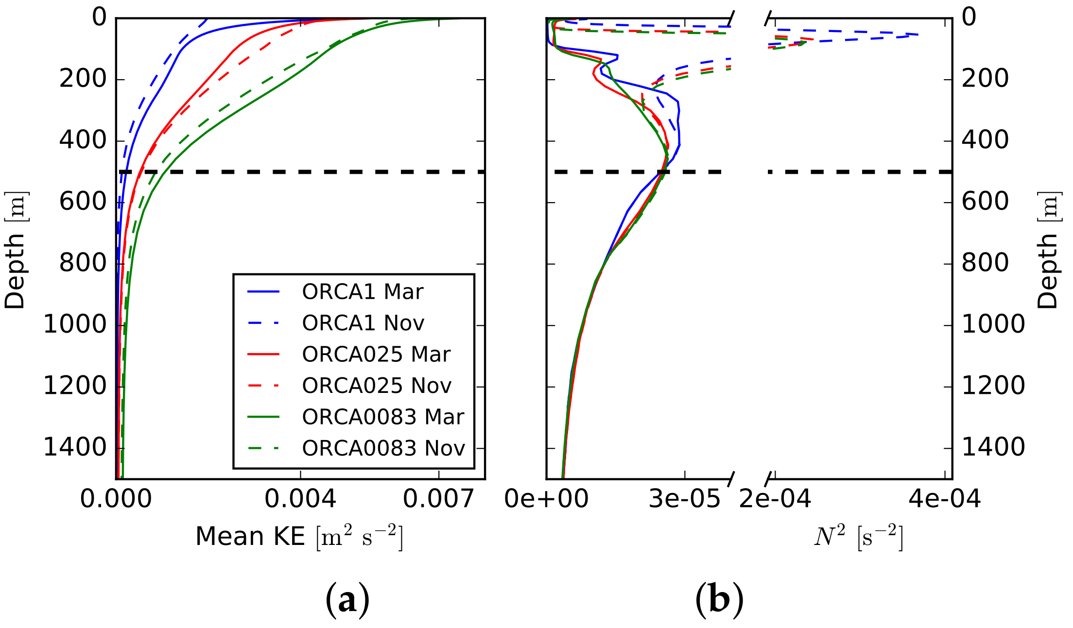
Figure 4.
(a) timeseries of root-mean-square (RMS) vertical shear in ORCA1 (blue), ORCA025 (red), and ORCA0083 (green); (b) RMS upper-ocean density anomalies for the Kuroshio region. Horizontal dashed lines indicate time average; (c,d) power spectral density in units and of the two time series in the top and middle figures respectively. Horizontal axis is , where t is time in days. Vertical dotted line shows annual frequency.

Figure 5.
Kinetic energy spectrum, , as a function of wavenumber, for ORCA1 (blue), ORCA025 (red), and ORCA0083 (green). Vertical lines show energy-containing scale, . Black vertical line shows first baroclinic Rossby radius, , in ORCA0083, although it is nearly identical in all simulations. Numbers show the result of a fit to determine p for between the energy-containing scale and the highest wavenumber.
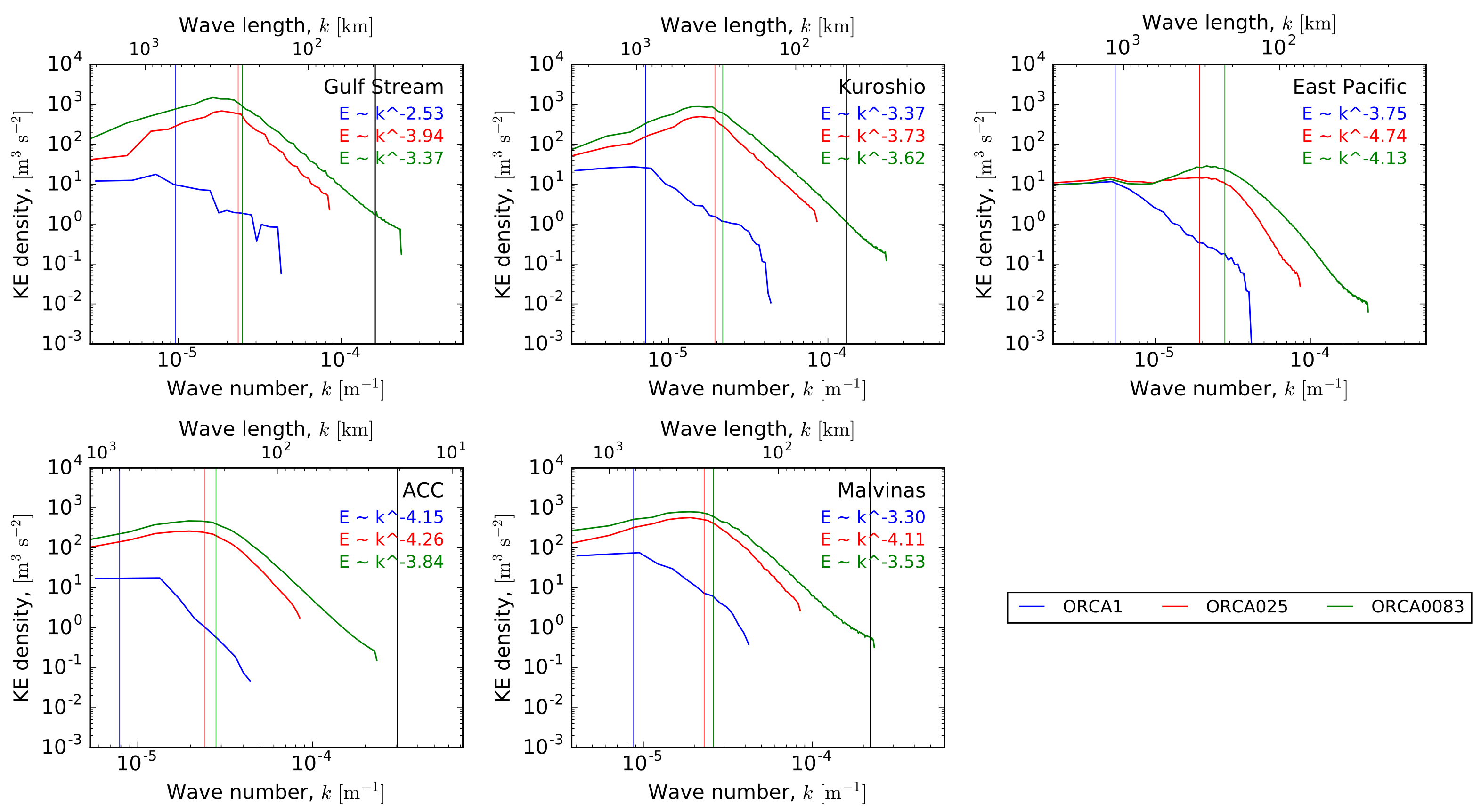
Figure 6.
Spectral flux for nonlinear interactions, , and pressure gradient, , (Equation (1)) for ORCA1 (blue), ORCA025 (red), and ORCA0083 (green). In the left figure, advection, , is solid, and pressure gradient, , is dashed. In the right figure, wind forcing, , is solid, viscosity, , is dotted, and bottom friction. Note the different vertical scale for the East Pacific region. Note also that spectral fluxes have units since they are the integrals of spectral transfers, which have units of kinetic energy (KE) tendency, .

Figure 7.
Spectral flux for baroclinic nonlinear interactions , (dashed lines, left panels), barotropic nonlinear interactions, (solid lines, right panels) and barotropisation, (dotted lines, right panels) for ORCA1 (blue), ORCA025 (red), and ORCA0083 (green). Note the different scales for the East Pacific region. As in Figure 6, note also that spectral fluxes have units since they are the integrals of spectral transfers, which have units of KE tendency, .

Figure 8.
Spectral fluxes for barotropisation, (blue), barotropic inverse cascade (red), barotropic bottom drag (green), and barotropic horizontal viscosity, (black) for ORCA025 (a), and ORCA0083 (b) in the Kuroshio region.
Figure 8.
Spectral fluxes for barotropisation, (blue), barotropic inverse cascade (red), barotropic bottom drag (green), and barotropic horizontal viscosity, (black) for ORCA025 (a), and ORCA0083 (b) in the Kuroshio region.

Figure 9.
Fraction of total KE (barotropic + baroclinic) that is in the barotropic mode for ORCA1 (blue), ORCA025 (red) and ORCA0083 (green).
Figure 9.
Fraction of total KE (barotropic + baroclinic) that is in the barotropic mode for ORCA1 (blue), ORCA025 (red) and ORCA0083 (green).

Table 1.
Parameters used for the ocean model simulations used in this study. The vertical coordinate is explained in the text. Note that the simulations have different forms of horizontal viscosity.
Table 1.
Parameters used for the ocean model simulations used in this study. The vertical coordinate is explained in the text. Note that the simulations have different forms of horizontal viscosity.
| Parameter | ORCA1-N406 | ORCA025-N401 | ORCA0083-N001 |
|---|---|---|---|
| Hor. res. | |||
| z levels | |||
| Time step, | |||
| Hor. visc. order, | |||
| Hor. visc., | |||
| Vert. visc., | |||
| Drag coeff., | |||
| Backgr. turb. KE, | |||
| Tracer diff., | |||
| Tracer diff. form | Iso-neutral | Iso-neutral | Iso-neutral |
| Eddy param. | Yes, [18] | No | No |
| Ref. density, |
© 2017 by the authors. Licensee MDPI, Basel, Switzerland. This article is an open access article distributed under the terms and conditions of the Creative Commons Attribution (CC BY) license (http://creativecommons.org/licenses/by/4.0/).
Share and Cite
MDPI and ACS Style
Kjellsson, J.; Zanna, L. The Impact of Horizontal Resolution on Energy Transfers in Global Ocean Models. Fluids 2017, 2, 45. https://doi.org/10.3390/fluids2030045
AMA Style
Kjellsson J, Zanna L. The Impact of Horizontal Resolution on Energy Transfers in Global Ocean Models. Fluids. 2017; 2(3):45. https://doi.org/10.3390/fluids2030045
Chicago/Turabian StyleKjellsson, Joakim, and Laure Zanna. 2017. "The Impact of Horizontal Resolution on Energy Transfers in Global Ocean Models" Fluids 2, no. 3: 45. https://doi.org/10.3390/fluids2030045