Hasegawa–Wakatani and Modified Hasegawa–Wakatani Turbulence Induced by Ion-Temperature-Gradient Instabilities


Institut Jean Lamour, CNRS UMR 7198, University of Lorraine, BP 239 F-54506 Vandoeuvre les Nancy, France
*
Author to whom correspondence should be addressed.
Fluids 2017, 2(4), 65; https://doi.org/10.3390/fluids2040065
Submission received: 9 October 2017
/
Revised: 4 November 2017
/
Accepted: 13 November 2017
/
Published: 23 November 2017
Abstract
:We review some recent results that have been obtained in the investigation of zonal flow emergence, by means of a gyrokinetic trapped ion model, in the regime of ion temperature gradient instabilities for tokamak plasmas. We show that an analogous formulation of the zonal flow dynamics in terms of the Reynolds tensor applies in the fluid and kinetic regimes, where polarization effects play a major role. The kinetic regime leads to the emergence of a resonant mode at a frequency close to the drift frequency. With the objective of modeling both separate fluid and kinetic regimes of zonal flows, we used in this paper a methodology for deriving both Charney–Hasegawa–Mima (CHM) and Hasegawa–Wakatani models. This methodology is based on the trapped ion model and is analogous to the hierarchy leading from the Vlasov equation to the macroscopic fluid equations. The nature of zonal flows in the hierarchy of the Mima, Hasegawa and Wakatani models is investigated and discussed through comparisons with global kinetic simulations. Applications to the CHM equation are discussed, which applies to a broad variety of hydrodynamical systems, ranging from large-scale processes met in magnetically confined plasma to the so-called zonostrophy turbulence emerging in the case of small-scale forced, two-dimensional barotropic turbulence (Sukoriansky et al. Phys. Rev. Letters, 101, 178501, 2008).
1. Introduction
Understanding and controlling turbulence is one of the key elements for a successful magnetic confinement of a tokamak plasma. Turbulence due to drift-wave is a ubiquitous feature of magnetically confined plasmas. In the studies of magnetized plasmas, theories and simulations have predicted that drift-wave turbulence or interchange turbulence [1], in the case of a toroidal geometry, can generate mesoscale structures, such as zonal flows (ZFs), sheared flows, but also streamers. These mesoscale structures, ZFs and streamers, have different behaviors and their impacts on turbulence-driven transport show strong contrasts. A spontaneous transition to a turbulence-suppressed regime is sometimes observed and is known as low-to-high (LH), confinement transition [2]. Streamers appear to be closely associated with avalanche-type transport events and contribute to enhancing the transport owing to their radial elongated structures. Motivated by the experimental discovery of the LH transition, experiment and theory in the last decade have focused on whether the turbulence associated with the H-states might be regulated by interactions with ZFs. The generation of ZFs and their feedback on turbulence itself by shearing turbulent eddies and/or drift wave packets have been studied in Refs. [3,4,5,6].
The theoretical understanding of ZFs and streamers has first come from studies on the drift-wave model but also in the gyrokinetic turbulence modeling [7], e.g., the ion temperature gradient (ITG) mode and the trapped ion modes (TIMs), thanks to the assumption of adiabatic invariance of the magnetic momentum and of the parallel kinetic energy of particles trapped in the so-called banana orbits [8,9], as well as gyro-fluid descriptions in a 2D or 3D space (see, e.g., Refs. [10,11]).
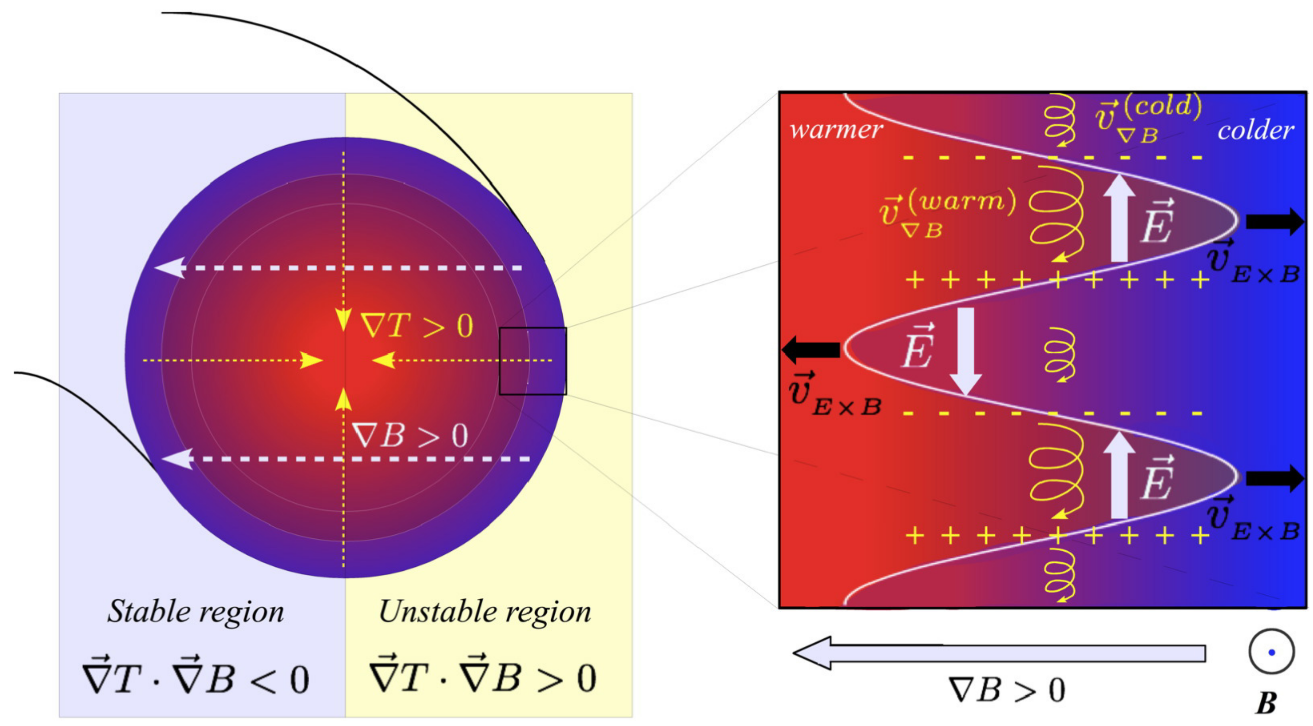
ITG modes are tokamak instabilities of interchange type (i.e., akin to the classical Rayleigh–Taylor instability in fluids), which determine the growth of perturbations in the poloidal angle because of charge separation effects due to an unfavorable radial variation of the so-called -drift particle velocity (see Figure 1). Since the latter is proportional to the particle kinetic energy component perpendicular to the local magnetic field, it depends on the particle temperature according to where T is the particle temperature in the poloidal plane, e is the particle charge and B is the amplitude of the magnetic field . While in a tokamak the plasma temperature is radially decreasing outward from the core of the vessel, the magnetic field intensity B, because of stability design, decreases in the direction opposite to the tokamak major radius (the intensity of the dominant toroidal magnetic field component being approximatively inversely proportional to the tokamak major radius ). As a consequence, the “outer” part of the poloidal section of the plasma with respect to the tokamak rotation axis has the gradients of both temperature and magnetic induction intensity pointing toward the axis. A perturbation in the poloidal angular direction will therefore mix the inner, warmer plasma, having a higher -velocity, with the outer plasma, colder and then relatively slower. This difference in the angular velocity corresponds to a charge separation and to an angular electric field component, which will foster the mixing of the warm and cold portions of the plasma because of two oppositely oriented -drift velocity components () along the radial direction.
A review of physics of ZFs can be found in Ref. [12]. The generation of ZFs was also predicted in the geostrophic vortex equation by Charney in [13] and by Hasegawa and Mima in Ref. [14] in the case of drift-wave turbulence. This model aims to capture the essential physics while involving the least number of scalar fields as possible, in order to get a deeper physical insight and in the attempt to unravel the complexity of the phenomena under investigation. In this context, great interest has been recently attracted by the two-field descriptions (involving ion density and vorticity) provided by the Hasegawa–Wakatani [15] (HW) and Modified Hasegawa–Wakatani [16,17] (MHW) models for drift-wave turbulence. They consist in a more complex formulation of the earlier and somehow simpler Charney–Hasegawa–Mima (CHM) model, successful in describing a wide variety of turbulent process, both in atmospheric fluids [13] and in plasmas [14]. On the other hand, barotropic instability is the atmosphere-ocean counterpart of plasma resistive drift-wave instability. In particular Charney in [18] showed that the CHM model may describe the regime of geostrophic turbulence pertinent to the largest planetary scales. Even in its simplified barotropic version (with infinite Rossby deformation radius), the commingling of strong nonlinearity, strong anisotropy and Rossby waves give rise to complicated dynamics (see for instance Refs. [19,20]).
ZFs are also met in natural phenomena and the physics of ZF formation was also studied within the geophysical fluid dynamics community. Recently, in CHM flows with a small-scale forcing, the simulations have shown that the inherent anisotropy inverse energy cascade can lead to a new regime of turbulence, referred as the zonostrophic regime [21], a particular regime of geostrophic turbulence as shown in [22,23]. This regime is characterized by an anisotropic spectrum, the formation of alternating zonal (east–west) jets and nonlinear (Rossby solitary) waves called zonons. These modes exhibit low frequency oscillations and display similarities with the resonant trapped-ion-mode (TIM) met in plasma physics. More recently, the data obtained from the Nasa spacecraft Cassini in Ref. [24] have shown that Jupiter’s troposphere in sharp contrast to the Earth’s atmosphere, conforms to the regime of zonostrophic turbulence.
While considerable progress has been achieved in the understanding of the zonal flow physics, many aspects of the ZF dynamics remain nevertheless poorly understand. The generation of ZFs and their feedback to turbulence and transport are essentially nonlinear processes. ZFs are non resonant and are generated through the Reynolds tensor in the drift-wave turbulence. A clear indication of the key role played by ZFs was the recent observation in Ref. [25] at the Experimental Advanced Superconducting Tokamak (EAST) or in the DIII-D tokamak in Ref. [26], associated with a low frequency signal at a few kilohertz, i.e., at a much lower frequency than the usual geodesic acoustic mode, the geodesic version of ion acoustic modes. Central to all these physical turbulent systems, be they in the core region of the tokamak plasma or in the shallow rotating atmosphere, is the generation of ZFs, exhibiting low frequency oscillations, which are believed to be responsible for suppressing small-scale turbulence and stabilizing the turbulence. This brings us to an important question about the physical origin of these low-frequency oscillations while the ZF frequency is usually attributed to be zero in the hydrodynamic approach. From the work described in Ref. [27], the answer appears to lie in the fact that the nature of the ZF is strongly modified by nonlinear effects induced by the resonant character of (kinetic) TIMs, at least for the case of turbulence met in tokamaks.
The kind of dynamics involved in all these systems has the same general structure, which explains the many qualitative similarities between the systems. In particular, in the case of the zonostrophic regime, the low frequency oscillations-referred as zonons- are interpreted as nonlinear perturbations which essentially depend on resonant triad interaction. This was theoretically predicted in Refs. [21,28] and can be recovered by a simple CHM model including a small-scale external driver. Even more surprisingly, the same general structure of the ZF, at least driven by the Reynold tensor, is found in the tokamak models of Hasegawa, Mima and Wakatani. As exemplified by the case of the study of zonostrophic turbulence, the possible occurrence of these nonlinear structures allows insight in the strong turbulence regime described by the CHM equation and in the role played by forcing term. However, although the reduced tokamak models of Mima, Hasegawa and Wakatani exhibit systematic deficiencies in representing the kinetic effects, since such effects are not included, accurate simulations of the ZF production require a correct representation of the resonant interaction energy transfer mechanism (in particular from small-scales).
In particular, the main interest in the HW and MHW models lays in their debated capability to account for a self-consistent generation of zonal flows by small-scale turbulence, and thus in the possibility to shed light in the spontaneous transition to a turbulence-suppressed regime. In this respect, these models display some differences.
While the feature of zonal-flow generation, driven by the Reynolds tensor, was already present in the fluid CHM framework, the CHM model seems to be inappropriate to describe the turbulence at small-scale without the introduction of an external forcing term. The HW model, which like the CHM model for plasmas evolves the ion vorticity (at the -drift ordering) and the ion density fluctuations, was developed to describe anomalous edge transport induced by collisional drift-waves. It contains a term more than the CHM model. This term is due to the electron dynamics parallel to the magnetic field, as it is deduced from Ohm’s law, and linearly couples the fluid stream function, i.e., the electrostatic potential, with the ion density. Such parallel electron dynamics contribution enters with a coefficient, which is usually named the “adiabaticity parameter”, since it measures the electron adiabatic response along the magnetic field lines. The MHW differs from the HW model because the zonal components have been subtracted from such a linear coupling, and a further contribution proportional to the background inhomogenous density (assumed to be constant in time) times the drift velocity is included. These corrections to the HW model have been included in Ref. [16] because it was mentioned that, without these terms, the original HW model was otherwise incapable of describing the zonal flow generation. This assertion, mentioned in Ref. [17] to be at odds with the CHM limit of the HW model and with the fact that the CHM, was in turn capable of describing a self-consistent zonal flow generation, was pointed out by numerical simulations of the HW model to be true only for small values of the adiabaticity parameter [17], for which both the MHW and HW models converge toward the 2D Navier–Stokes equation.
Thus, we need a reference model for generation of ZFs and their impact on the turbulence suppression that allows to characterize the nature of ZFs generated in the different reduced models such as CHM, HW and MHW. The Hamiltonian trapped ion model is a very useful and instructive model, even if restricted to plasma physics. The results from the reduced Hasegawa, Mima and Wakatani models also have to be regarded with some caution because the nature of ZFs depends on the effects at play in each model. A particularly insightful way to utilize and compare these reduced models is to examine the interactions of the drift-wave (or interchange-type ) turbulence with ZFs, by starting from the global trapped ion model.
In this paper, we address these points by providing a rigorous derivation of a MHW-type model from a reduced kinetic model for trapped ions in banana orbits, apt to describe the production of ZF through a resonant energy transfer mechanism [1,8,9]. The trapped ion model can be seen as an extension of the HW model, and allows the description of TIMs, a prototype of collective modes of kinetic nature. This model allows a fine description of the interchange turbulence in which the resonant interaction between TIM and trapped ions takes place through the precession motion of the latter. In revising the hierarchy of CHM, HW and then MHW models, we will address how this hierarchy is linked to a closure condition obtained from the kinetic model, which allows us to recover the Reynolds tensor shear effects only in the HW approach, a mechanism that may impact the turbulence.
The MHW-type model differs however from the one proposed in Ref. [16], to which it will be compared together with the HW model of Ref. [17]. We then discuss the physical limits in which the kinetic equations reduce to the HW and CHM model, and we finally discuss some properties of the MHW set we have described. In particular, we present numerical results obtained from integration of the reduced kinetic, Hamiltonian gyrokinetic model for the trapped particles [9] based on an action-angle model first discussed in Ref. [8], which corresponds to a simplified version of the upgraded version called “TERESA”, by referring to one of its numerical parallel hybrid (OpenMI—Message passing Interface) implementations [29] to describe the process of the ZF formation.
2. Hamiltonian Model for Ion Temperature Gradient (ITG) Turbulence
The model, we consider for a tokamak plasma, describes the dynamics of TIMs in which the gradient of temperature gives the source of free energy. TIMs play a major role in the range of frequencies that is well below the parallel transit frequency. TIMs are then obtained by averaging the particle dynamics over fast scales, that is, over the cyclotron and bounce motions in the toroidal geometry. This task is made easier in the framework of the Hamiltonian–Jacobi formalism using action-angle variables. Due to their curvature drift, the orbits of trapped ions in a tokamak display a “banana” shape centered on the low magnetic field side. The low-frequency response for TIM is obtained by making a phase-angle average over the cyclotron phase and the bounce motion. This is allowed by the invariance of the total energy and of the so-called adiabatic invariant , which is appropriate at the time scales of interest for this problem. Here, the label G is a conventional notation which refers to the guiding centre and refers to polar coordinates. In agreement with the experimental conditions, we consider low values and a poloidal field lower than the toroidal magnetic field . The modulus of the magnetic field is given by where is the minimal value of the magnetic field amplitude B at ( being then the major radius and the minor radius). In this configuration, the action-angle coordinates of the trapped particle distribution are the precession angle and the poloidal flux . The poloidal flux is related to the poloidal field by and , where q is the safety factor and is the inverse aspect ratio. The precession angle is related to the toroidal and poloidal angle coordinates by . The gyro-average operator is approximated by Pade’s relation (see Refs. [30,31]):
This operator introduces a “banana” scale corresponding to the width of the particle’s trajectory in the direction, while the gyro-phase average on the Larmor radius acts along the direction of the precession angle . Rather than working with the adiabatic invariant , it is interesting to introduce the pitch angle parameter defined by the relation where . The use of the pitch angle , rather than , will allow us to characterize ions in the form of trapped populations () or of passing particles (). Following the work of Kadomtsev and Pogutse [32], the bounce and precession frequencies are respectively given by the following relations:
where is the magnetic shear. and are the complete elliptic integral of the first and second kind, respectively. Trapped ions in a banana orbit are described by two invariants, the energy E and the pitch-angle , and by the distribution function fulfills the Vlasov equation:
with the advective-term depending on the gyro-average operator defined in Lable (1) and expressed by means of the Poisson brackets . The right-hand-side (RHS) expresses numerical particle diffusion (see the end of the section). The polarization effects have been taken into account in the quasi-neutrality equation by the introduction of the polarization density (the Laplacian term). This is due to the difference between the real trapped particle density and the bounce-averaged banana centre density. Assuming an adiabatic response for electrons, the quasi-neutrality condition , where and are the fluctuations of the particle densities, reads:
Here, is the equilibrium density, equal for both ions and electrons. The operator , which describes polarization effects, introduces the spatial scales and . The first term on the left-hand side of Equation (5) comes from the adiabatic condition of electrons while the second term is due to the polarization charge. The gyro-averaged ion density is obtained by replacing the distribution with in the expression of the ion density, , defined by
and are constants accounting for , the fraction of trapped particles, and for the ratio of ion to electron temperatures, and . Trapped ion turbulence develops on a length scale of the order of the banana width and on a time scale determined by , where . Here, is constant since we have neglected the dependence in and is found to be close to . In Equation (4), the diffusion coefficient is introduced for numerical purposes. In practice, in the numerical code, this diffusion coefficient is set to zero everywhere, except in a small buffer region located on the boundaries of the numerical box at and . This choice allows to control the level of turbulence on the box boundaries (the buffer regions occupies less than 10% of the radial domain, in which a small diffusion process is applied with a constant coefficient ). In what follows, we will focus on the domain of interest, namely the core turbulent region where D is zero.
It is interesting to recall here some general properties of the linear analysis of TIMs. By linearizing Equations (4) and (5), for an equilibrium distribution given by Equation (28) of Section 5, one obtains, by considering a standard potential perturbation mode in the form , the following relation:
with the usual Landau prescription on the imaginary part of . Note that, in Equation (7), we have neglected the polarization term in first approximation. As first noted in Ref. [33], a convergence of the expansion for the pole’s calculation in Label (7) can be obtained by considering a development around leading to an estimation of the collisionless TIM frequency in the form (with ):
where we have taken the average over the and E variables. Here, is the electron diamagnetic frequency, is the wave vector (for the variable ) and is the ion Larmor radius. Thus, it is possible to excite an oscillating ZF component when the last term in (8) becomes of order of . We then have
In Equation (9), the resonant amplification is produced by a three-wave process in which an interchange mode (of frequency and of toroidal number n) decays into a resonant collisionless TIM (of frequency and of toroidal number n) and a ZF (with a zero toroidal number).
3. Recall of Previous HW, MHW-Type and CHM Models for Drift-Wave Turbulence
In the following, we are going to show the connection between the Hamiltonian model of Section 2 with HW- and MHW-type equations. Before deriving the specific form the latter takes in this framework, we recall the HW and MHW-type formulations which have been proposed in two previous works [16,17]. They consist of a two-field theory involving the ion vorticity and the ion density fluctuation, which in our notation reads , by assuming that . In the coordinate system and in the non-viscous regime we consider, the MHW formulation proposed by Numata et al. [16] reads
where , and is the adiabaticity parameter that depends on electron-ion collisions through the resistivity , and on the toroidal wave-length component related to the poloidal scale length by , being the maximum angle . The main difference with respect to the HW modelling (In a three-dimensional system, the distinction between the HW and MHW models disappears and the “adiabaticity parameter” is not a constant, but rather an operator proportional to . However, since we are interested here in the radial contribution of the turbulence and not in the high-frequency contribution induced by high-frequency geodesic adiabatic mode (GAM) in zonal flow (and usually triggered by circulating particles), a two-dimensional approach is sufficient. Here, we have introduced the term “low-frequency” zonal flow (LFZF) to discriminate between the quasi-zero zonal flow (due to the Reynolds tensor) and the high-frequency GAM.) lays in having taken out the averages over , so that the quantities and express the potential and ion density fluctuations, respectively. The parameter is the normalized gradient of the density equilibrium profile, . The particle flux in the direction can be generated by out-of-phase fluctuations of and in and depends on itself, according to
This acts as a source term for the conservation of the energy E of this MHW model (label in the time derivatives below),
and of the enstrophy ,
The unmodified HW set of equations, which has been considered by Pushkarev in Ref. [17], consists instead of the equations
Differently from Equations (10) and (11), besides the absence of the last term on the right-hand-side (RHS) of the density equation, the coupling term does not depend on averages over the -coordinate. Labeling with “”, the time derivatives of the energy and enstrophy in this unmodified HW model, they obey
4. Applications to CHM and HW Turbulence
At this point, we would like to come back to the observation of Numata et al. in Ref. [16], of fast emergence of ZF in the MHW model. It was claimed by these authors that the original HW model does not predict the formation of ZFs, which appears to be in contradiction with the CHM results of Connaughton et al. and reported in Ref. [34], considering the fact that the HW model includes the CHM model as a limiting case. We discuss here the importance of addressing the problem of drift-wave turbulence in the framework of the reduced Hamiltonian model for trapped particles, in order to gain a better understanding of the differences between the HW and MHW models. One of our objectives is to find a rigorous justification for the nature of ZF observed in the different models. This requires one to obtain a self-consistent dynamics equation. The problem is related to the choice of the closure condition whose origin comes from the nonlinearity and from the kinetic nature of the trapped ion model we consider. We choose to start with the CHM model.
4.1. The CHM Model
Assuming a homogeneous equilibrium density in (a choice to simplify the presentation), it is possible to recover a CHM- type equation from Equation (A4) in the following form (see Appendix A for details):
Note that now Equation (19) includes a source term at RHS due to the presence of the ion pressure. However, this term disappears when we consider its average over . From (19), it is clear that the nature of the ZF is purely driven by the term . Thus, by expressing the Poisson bracket in standard form, we find, after averaging Equation (19) over and after integrating two times over ,
which clearly indicates that the nature of the emerged ZF is driven only by the Reynolds tensor. The similarity between the reduced Hamiltonian model for trapped ions and the CHM equation had been already pointed out in Ref. [1].
4.2. The HW and MHW Model
The HW equation can be obtained with a similar analysis. By integrating Equation (A5) over and by replacing by , we obtain
Using the quasi-neutrality Equation (5), a little algebra leads to
Formula (A7) leads to
Some remarks are due:
- (i)
- In the MHW, the mean coupling function is given by which is strictly zero. This indicates that only the Reynolds tensor plays a major role in the generation of the ZF since in that case the second term in the RHS of Equation (24) disappears and, as a consequence, both CHM and MHW models are equivalent as far as the emergence procedure of ZFs is concerned.
- (ii)
- In the HW model, as shown in Equation (24), there are two basic effects in the dynamics: the first term at RHS shows the growth of ZF induced by the drift-wave turbulence (via the Reynolds tensor) while the second term indicates the possibility of the suppression of turbulence by a ZF shear mechanism, which takes place at a larger scale in the space. Rather than proceeding scale by scale in a local manner, energy transfer is here induced by competing processes between the smallest and the largest scales. Thus, the strong growth of ZF is expected and usually observed in both CHM and MHW models, whereas the suppression of drift-wave turbulence induced by a ZF shear is only expected in the original HW model, provided that .
4.3. The Kinetic Nature of ZF Driven by TIM
In the TIM model, it is also possible to connect the time variation of of ZFs to the ion pressure fluctuations, here driven by an interchange-type turbulence, a physical mechanism which is absent in the HW model. Since the model has been already derived in a previous work [27], we just recall here the main features relevant to the ZF dynamics. Assuming that is zero, in order to simplify the treatment, we just consider an ITG instability driven only by an initial temperature gradient, which corresponds to suppressing the second term in (24). We focus here on the effects induced by the ion pressure on the ZF dynamics. The evolution of the ZF is now described by the following equations:
assuming that there is no dissipation (i.e. ) and where
In Equation (25), the first term at RHS denotes the Reynolds tensor, while the two following terms are a straightforward consequence of the kinetic effects. The third term at RHS of Equation (25) is linked to the heat flux defined by Equation (26).
In a similar way, a mean ion pressure is also driven by nonlinear processes. Assuming that the gyro-average operator and , and that the second order effects (i.e., the second moment in energy of the distribution function ) are negligible, the mean pressure obeys an equation expressing, on average over , a Lagrangian advection by the flow (see Ref. [27] for more details):
It is worth pointing out at this stage that choosing equal to zero in Equation (25) leads to the HW model expressed by (24) in the case of an homogeneous equilibrium density. Formula (25) makes evidence of a role of the Reynolds tensor, wider than it is usually evidenced in fluid HW-type models. In particular, this expression shows that the ZF is impeded by the resonant interaction with collisionless TIMs, leading to a low-frequency ZF mode with a frequency close to .
Furthermore, when adiabatic conditions set in (or, equivalently, when ), from (5), we have . The last term comes from the average operator . Thus, in the case of an adiabatic system, we have ) and the expression of the zonal flow reads .
5. Numerical Simulations
In this section, we discuss the results of numerical simulations performed in order to elucidate some of the key features of the interchange turbulence in the presence of TIMs.
Our numerical scheme is based on the integration of Equations (4) and (5) in a self-consistent way. The numerical algorithm is based on a semi-lagrangian scheme detailed in Ref. [14], allowing the integration of the distribution function directly in phase space. It is worth noting that a semi-Lagrangian scheme was also applied in [35] to improve the efficiency of numerical models of the atmosphere. Such a numerical scheme allows an accurate integration of the Vlasov equation along its characteristics. The code employs a classic time splitting scheme to separate the treatment of the advection due to the drift-frequency but uses a full 2D advection in space to treat the advection due to the electric potential. It must be pointed out that semi-Lagrangian Vlasov simulations are slowly introduced in place of the well-known Lagrangian particle-in-cell simulations for two main reasons: the lack of numerical noise (in the sense that, in the Eulerian approach, the graininess parameter tends to zero and where is the Debye length and the particle density) and the very good resolution of the distribution function in phase space provided the dimension of the momentum space is as lowest as possible (depending on the computational constraints).
We focus on the nonlinear generation of ZFs by varying the parameter related to polarization effects. Equations (4) and (5) have been solved using a backward semi-Lagrangian scheme [36]. Semi-Lagrangian Vlasov simulations have identified two different kinds of ZFs of somewhat different nature, the first kind of ZFs driven by the Reynolds tensor, as expected, in agreement with the results of the standard fluid HW model. The second type of ZFs is characterized by the resonant coupling with TIMs, a physical process that is not taken into account in the reduced HW model.
In numerical simulations, quantities are normalized as follows: the time is normalized to the inverse drift frequency , the poloidal flux is given in units (with ), the energy E is normalized to . The electric potential is expressed in units and the constants and introduced in the quasi-neutrality Equation (5) are given by the relations and . The bounce and drift frequencies and depend explicitly on the pitch angle parameter (and of course on the energy E) and are given by Equations (2) and (3). The initial distribution function is given by:
In Equation (28) the quantity denotes the initial flow corresponding to the interchange case. Here, is the normalized ion temperature gradient. The starting point for an investigation of interchange turbulence is the reduced gyrokinetic Vlasov Equation (4) coupled with the quasi-neutrality equation condition (5) initiated in an equilibrium state with a perturbation term of type:
The reason for introducing the factor in Equation (29) on the right-hand side instead of the standard potential perturbation in is that this function is the marginal solution obtained in the linear analysis of the TIMs. Here, we choose a perturbation on the potential .
Without dissipation, three energetic subsystems interact to produce the complexity observed in the interchange-type turbulence: the kinetic energy of the plasma
the energy of the zonal flow noted here by
and the potential fluctuation of turbulence
Here, we have studied in detail the effects of the polarization term. A series of simulations has been performed for different values of the parameter the other physical and numerical parameters being kept constant. In all simulations presented below, we have taken an ion temperature gradient of , chosen above the threshold of the ITG instability given by , for and a banana width of . We choose a Larmor radius of and a magnetic shear of , well inside the region of strong ITG instability. The phase space sampling is given by and points and we have used values in pitch-angle and energy. The time step is . The time evolution of the different energies is plotted for in Figure 2, in correspondence with non-negligible values of the electric potential.
We choose to start with a small value of , i.e., well inside the Reynolds’ tensor-dominated regime. Results are presented, in the top panel of Figure 2, the time evolution of the zonal flow energy (in red and in solid line) together with its turbulent energy counterpart (in blue and in dotted line). As shown in Figure 2, the dynamics of the plasma are first governed by the growth of turbulence, as a result of the ITG instability. Here, it is the gradient in temperature that constitutes the energy source for the growth of TIMs, when the temperature gradient exceeds a critical value of . The case of an initial density gradient and of a resulting shear flow generated by a Kelvin–Helmholtz instability was presented in Ref. [37]. Here, the instability linked to a density gradient is not excited in the linear phase of ITG, but can appear later when nonlinear effects take place leading to the generation of shear flows. Note that at the saturation of ZF, in top panel in Figure 2, the turbulent component of the energy has strongly decreased. In the bottom panel in Figure 2, the corresponding evolution of the zonal flow component , taken at (in unit), is plotted in a logarithmic scale. Aside from the fast oscillation in the linear phase (linked to the linear TIM), no oscillatory behavior is observed in the saturation regime, a signature of the role played by the Reynolds tensor in the fluid regime.
We will now address how ZF is modified in the kinetic regime by its coupling with TIMs leading to a low-frequency oscillatory behavior, a mechanism that is different from the standard Reynolds stress met in hydrodynamics, and which is not taken into account neither in the HW model, nor in the MHW model. A second simulation is performed with . Results are shown in Figure 3 to be compared to those used in Figure 2. There is a qualitative change in the interchange turbulence, which now exhibits low-frequency oscillations just before the resonant amplification of the ZF component.
Zero-frequency ZF is quite non resonant and it is relatively easy for the Reynolds tensor to drive it up in a nonlinear way. While ZFs back-react upon turbulence by shearing, so weakening the source of their generation, it was shown in Ref. [37] that Kelvin-Helmholtz (KH) instability may act as a damping mechanism for ZFs. However, this latter mechanism becomes inefficient when the nature of ZF is modified leading to a time-varying ZF, which becomes now sensitive to resonant amplification through parametric three-wave scattering. Thus, a transition from the fluid regime to a kinetic one for ZF is expected when the polarization increases. Here, the LFZF generation is a nonlinear process in which shorter-scale fluctuations transfer their energy to larger-scale potential structures. In addition to the first phase of growth of TIM turbulence (), the nonlinear interaction leads to the growth of an oscillating mode on a frequency close to the drift frequency .
Such a behavior can be observed in the intermittent regime of turbulence and is usually associated with a turbulence burst. In order to illustrate the rich nonlinear dynamics that underlie the resonant amplification of ZF, we have performed a new numerical simulation over a long time, for the same value of the polarization parameter , but by diminishing the initial perturbation level of the potential by a factor ten, in order to follow the time evolution of the system in the (strong) intermittent regime of turbulence. This time, the time step is smaller, the phase space sampling is (here, we have reduced the sampling in to ) and we have used values in pitch-angle and energy. Numerical results are presented in Figure 4, Figure 5, Figure 6 and Figure 7. On the top panel in Figure 4, we have plotted the temporal evolution of the energies of the zonal flow component (in red and in solid line) and of the turbulent component (in blue and in dotted line). The zonal flow energy displays three different stages during its evolution: a first phase characterized by a weak growth-rate for , followed by a first resonant peak at and finally a second resonant process, now located at time , leading to a slow reduction of the turbulence after this time. On bottom panel in Figure 4, the temporal evolution of the mean potential is represented in a logarithmic scale: we see clearly the emergence of different behaviors during the time evolution. While the beginning of the simulation is characterized by high-frequency oscillations (due to TIMs), followed by the bursting behavior at a lower frequency, the oscillatory behavior disappears, at saturation, indicating that a fluid-type regime is now recovered and dominated by the Reynolds tensor.
Figure 5 shows the spectrum in frequency of the electric potential for the considered numerical simulation (over the total time and at a fixed point ): we observe clearly both components of ZF, the quasi-zero part driven by the Reynolds tensor and the oscillating component , at a frequency close to , a somewhat higher value than the predicted value of (using a magnetic shear of ). It must be pointed out that the resonance takes place for the dominant streamer mode, i.e., . Indeed, both mode and its harmonics are excited, as can be seen in Figure 5, where we have plotted the electric potential. This feature resembles the excitation of the nonlinear zonon mode, usually triggered by the same zonal wave vector of Rossby–Haurwitz waves (RHWs). In Figure 5, we observe also the growth of the mode and of its harmonics . In the linear regime, the frequency of TIM is reduced to a value of . However, TIM can propagate in the direction of the precession motion of ions allowing strong resonance with precessing ions: therefore, a slow decrease of TIM frequency is also possible when nonlinear trapping effects are important. Such a process has been already predicted by Morales and O’Neil in [38]. Thus, due to strong nonlinear effects, the frequency of the kinetic mode , initially close to the (linear) value can slowly decrease to reach a value close to , which finally leads to an estimation, for the ZF frequency, of . It is this way that harmonics of ZFs can be excited.
Figure 6 shows the behavior of the electric potential at three different times when the resonance takes place, showing clearly that, in the asymptotic regime, the dominant modes are and . We have therefore identified a nonlinear coupling of ZF mediated by nonlinear collisionless TIMs, leading to a strong reduction of the interchange turbulence.
In Figure 7, we have represented the mean ion pressure , as a function of the poloidal flux , and the corresponding electric potential at two times: the formation of a transport-barrier region (located around , where the temperature gradient becomes negligible, is made evident. This also indicated that the ITG instabilities are now strongly reduced in this region. Here, it is the polarization source that triggers the barrier and reduces the level of turbulence (see Ref. [39] for more details).
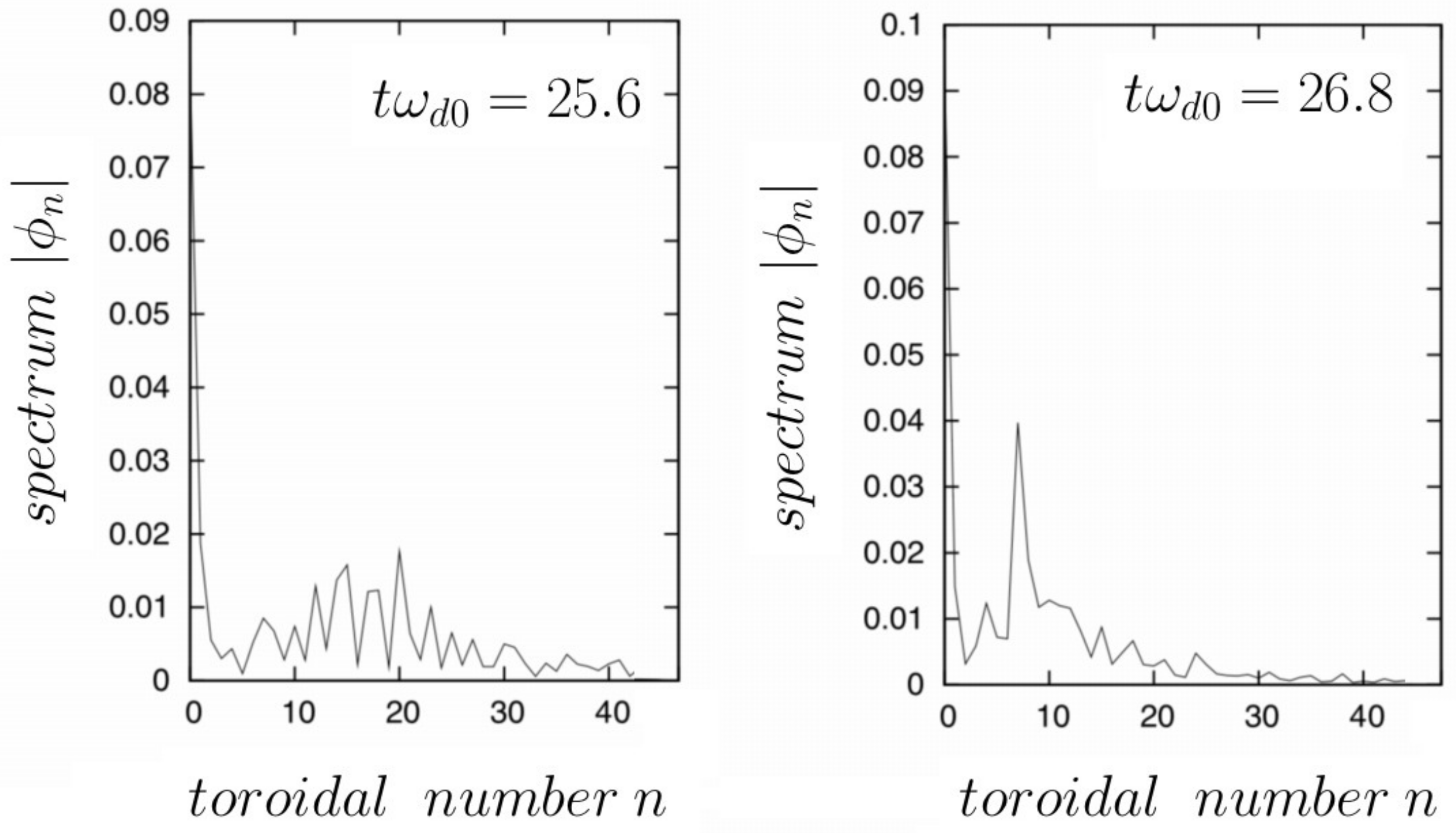
The last example, shown in Figure 8, Figure 9 and Figure 10, describes the dynamics of the resonant mechanism in an accurate way, when we increase the polarization parameter to a value of , i.e., well inside the kinetic regime of ZF. The numerical simulation was carried out using the same physical and numerical parameters of Figure 2 and Figure 3. We now focus on the transition toward the kinetic regime of ZF, which is triggered by the resonance of TIM wave with precessional trapped ions. An intermittent regime is observed (as expected in the dynamics previously shown in Figure 4) and we focus here on the dynamics just before the occurrence of the first burst, when the nature of the ZF is modified. On the bottom panel in Figure 8, we have plotted the electric potential, in a logarithmic scale, as a function of time. The oscillating nature of the ZF is clearly visible, even at saturation. In this saturation phase, ZF manifests as linear TIMs with a frequency and no frequency shift. The turbulent energy density peaks at the small n modes. These modes harbor the most energetic TIMs in the system. This mechanism is analyzed in more details through the phase space diagnostics shown in Figure 9 and the spectra in wave-numbers (i.e., in toroidal numbers) are plotted in Figure 10. Figure 9 illustrates the details of the electric potential, when the resonance takes place: we observe clearly the formation of streamers (i.e., nonlinear structures elongated along the direction). The intermittence is characterized by the generation of a turbulence burst at time , as the result of the emergence of the resonant TIM with toroidal number (note that the initial perturbed mode has disappeared at that time). Diagrams in Figure 10 reveal the occurrence of (nonlinear) streamers with a broad spectrum (with a toroidal number of n∼ 16–24), as can be seen in the plot shown at time . At time , an inverse cascade takes place leading to a dominant mode on the toroidal number , as indicated in the bottom panel in Figure 9.
6. Connections with the Zonostrophic Turbulence in Geophysical Fluid Dynamics
It is well known that the CHM equation and the quasi-geostrophic equation have the same structure. This makes it possible to establish a direct link between drift-wave turbulence in magnetically confined plasmas and the quasi-geostrophic turbulence in geophysical fluid dynamics (GFD). Both systems are approximately two-dimensional respectively because of the strong guide field applied to a magnetized plasma and because of the fast planetary rotation and strong density stratification in the quasi-geostrophic limit. Curiously, the same symbol is used, although with completely different meanings, to characterize both the strong-guide field limit in a plasma and the regimes of quasi-geostrophic turbulence. As already recalled in the introduction, in a plasma, labels the ratio between the kinetic and magnetic pressure, and it is small in the strong guide field approximation. In a tokamak, for example, for which an approximated two-dimensional description for the poloidal dynamics is allowed by the strong toroidal (guide) magnetic field, typically . On the other hand, in geostrophic turbulence denotes the ratio where and R are the angular velocity and the radius of a rotating fluid spherical shell. As mentioned earlier in the introduction indeed, computer simulations of 2D barotropic turbulence on a -plane surface of a rotating sphere gave rise to a classification of flow regimes, which become possible in these geostrophic systems, depending on the value of . One of these is the regime of zonostrophic turbulence, which is characterized by an anisotropic inverse cascade and by slowly varying structures of strong alternating zonal jets. The barotropic vorticity equation (on the surface of such rotating sphere) is then given by
where is the vorticity, is the stream function with , is the Coriolis parameter (the planetary vorticity), is the latitude and the longitude. In (34), the Jacobian J is defined by . is the hyper-viscosity coefficient and p the power of the hyper-viscous operator ( is usually used) and is the linear friction coefficient that expresses the large-scale friction. In Ref. [22], the authors have considered, in the CHM model, a small-scale forcing term S that pumps energy into the system at a constant rate and that leads to a new regime of the geostrophic turbulence, the so-called zonostrophic regime. However, no justification on the origin of such source term in the forced CHM model was given. The development of this new regime of turbulence is characterized by the existence of a new class of nonlinear waves dubbled zonons.
Indeed, Equation (34) can be solved using the decomposition of the stream function in spherical harmonics , leading to a class of linear Rossby–Haurwitz waves (RHWs) of frequency given by
Fixing the reference unit of length so that eliminates the difference between the indices of the spherical harmonics and wave numbers. The decomposition takes the usual form
where and are the meridional and zonal wave numbers, respectively (and N a truncation index). It must be pointed out that we have kept here the notation for the standard toroidal and poloidal numbers, respectively, and that the roles of and are inverted to tokamak’s with respect to toroidal geometry since refers to zonal jet while represents ZF in magnetically confined plasmas.
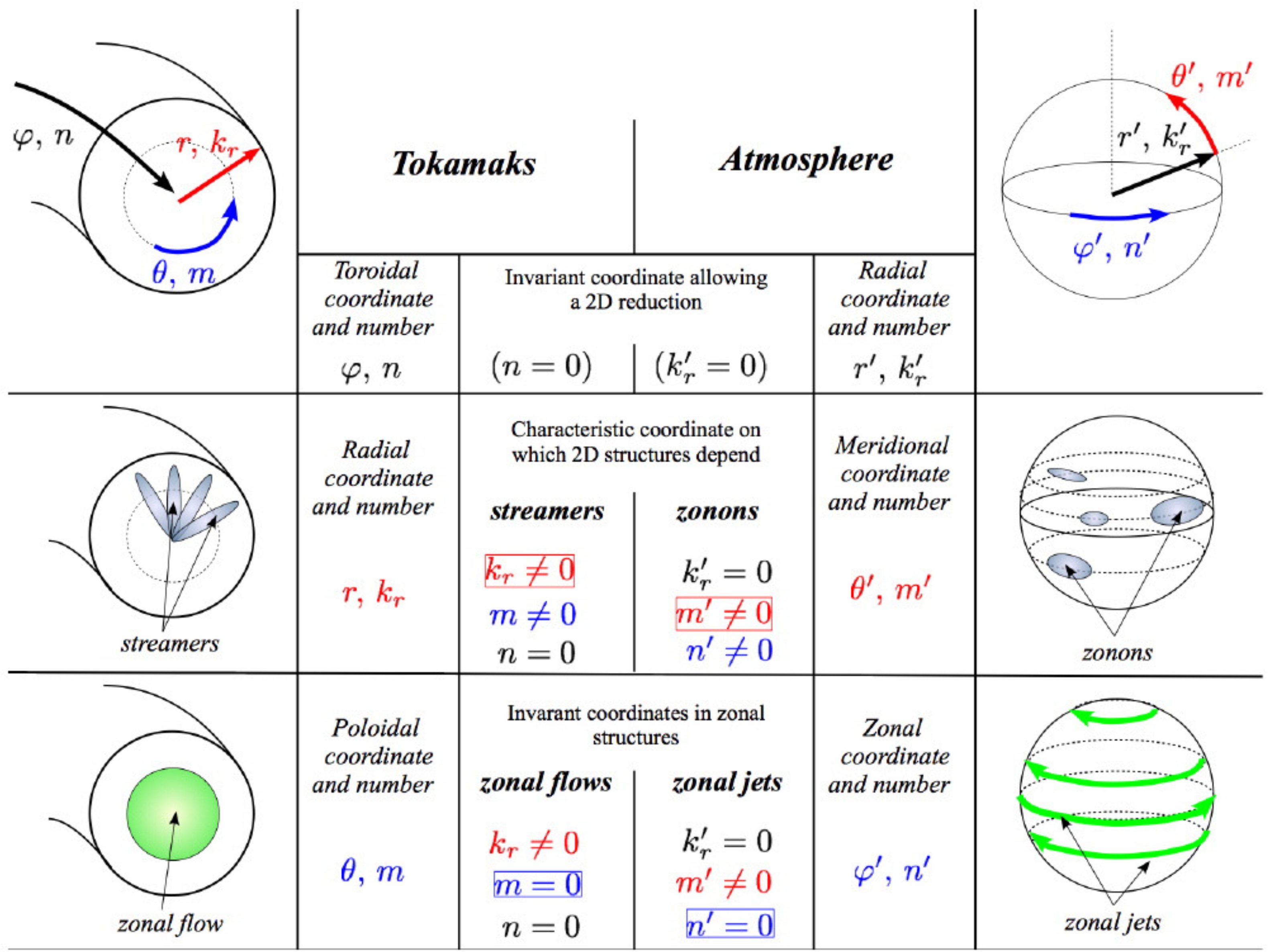
We recall indeed that, in the 2D description of drift-kinetic turbulence in a tokamak, the restriction to a planar geometry corresponds to the condition, which holds for both zonal flows and streamers. In the 2D description of zonostrophic turbulence the restriction to a 2D geometry is given instead by the condition . The correspondence between the set of toroidal coordinates in drift-kinetic turbulence in tokamaks and the set of spherical coordinates in zonostrophic turbulence in the atmosphere, also with respect to the zonal and nonlinear structures encountered in the two frameworks, is summarized in the scheme of Figure 11.
The situation observed in the zonostrophic regime resembles the situation met in previous sections where LFZF is generated (see Table 1 in which we have summarized the different waves implicated in the turbulent processes). We can say that, while ZFs are met in both plasmas and in the atmosphere, streamers in poloidal plasma turbulence are the correspective of zonons in zonostrophic turbulence. Our investigation reveals that, in tokamak turbulence, it is the small-scale wave-particle interactions (or nonlinear streamers) that determine the resonance conditions of the residual LFZF. Thus, a key physical point is that this low-frequency ZF can be excited by resonant triad. Moreover, in Ref. [28], the authors have proposed that RHWs can produce ZF through an energy transfer mechanism, triggered by resonant triads. Thus, the turbulence is here dominated by waves that are involved in triad interaction. What is more interesting is that, in the zonostrophy turbulence, the zonon frequency is equal to the frequency of the most energetic RHWs (by fixing a value of ) that excite zonons, as shown in Refs. [21,22,23,24,28,40,41]. In particular, is proportional to , a feature which exhibits a similarity to the property of linear resonant kinetic (TIM) modes (note that streamers are the nonlinear version of TIM) . Thus, the relationship between both types of waves is quite straightforward. Concerning the LFZF generation, there exists also, in the zonostrophic regime, zonal zonons with a frequency whereas for all values of the meridional wave numbers.
Finally, we would like to comment on the relation between the CHM equation given in (19) and the trapped-ion model. Nonlinear small-scale effects are here introduced, in the right-hand-side member, which indeed disappears when taking the average over the variable. This property shows that ZF is not affected by this term. It is not the case of the small-scale forced version of the CHM used in the study of the geostrophic turbulence: along with the linear RHWs, nonlinear small-scale structures (zonons) also emerge and an intense energy exchange between zonons and the ZFs can take place.
7. Conclusions
In reviewing some recent results about the emergence of zonal flows in the ITG-instability-driven turbulence in tokamak plasmas, we have compared a kinetic model for the description of TIMs with fluid CHM and HW-type models for turbulence. We have shown that the zonal flow generation in collisionless plasmas is controlled not only by the Reynolds tensor, usually recognized as the main actor in the fluid approach, but explicitly depends on the microscopic physics that govern the ion temperature gradient instability. We have found that the Hasegawa–Wakatani model can be recovered from the gyrokinetic trapped ion model when interchange-type turbulence is considered, and that the zonal flow dynamics is strongly impeded by polarization effects. It is the Laplacian operator acting on the electrostatic potential that determines the transition between a turbulent regime dominated by the Reynolds tensor and a new regime of kinetic nature, where streamers and shear-flow-driven vortices develop inside a low-frequency oscillating zonal flow. In this investigation, the use of a reduced HW model, or its modified version, has been particularly fruitful since, on the one hand, it contains the physics related to the Reynolds stress, a feature that is thought to play a fundamental role in the ZF emergence, and, on the other hand, it exhibits mathematical properties that allow us to make connections with the gyrokinetic trapped ion model in a rather compact and general form. The feature of ZF dynamics that we have discussed appear to be of quite general interest, as they are relevant to physical processes that take place in other natural systems, in particular in the zonostrophic regime of planetary atmospheric turbulence. This research will hopefully help to understand whether kinetic effects, occurring at small spatial scales, concur to the onset of zonotrophic turbulence regimes.
Acknowledgments
The authors are in debt to the IDRIS computational center, Orsay, France, for computer time allocation on their machines. This work was granted access to the high performance computing (HPC) resources (Grant 2014-2015-054028) made by Grand Equipement National de Calcul Intensif (GENCI).
Author Contributions
Alain Ghizzo performed numerical simulations. Daniele Del Sarto and Alain Ghizzo have developed the analytical model, interpreted the results and wrote the paper.
Conflicts of Interest
The authors declare no conflict of interest. The founding sponsors had no role in the design of the study.
Appendix A. MHW-Type Equations from the Hamiltonian Model
In this appendix, we show how, taking the zeroth velocity moment of Equation (4) and assuming the quasi-neutrality condition (5) and a diffusion coefficient D which tends to zero, we obtain for the zero-order moment of f in velocity:
Here, the ion density is given by (5) according to
by assuming that or, equivalently, that the gyro-average operator is approximated by the identity. In Equation (A1), the ion pressure is defined by
This rapid overview gives us an idea about how the HW emerges from the kinetic theory. In the HW approach, precautions have to be taken with the closure condition, since, in the set of Equations (A1) and (A2), the pressure is not known. Thus, by injecting (A2) into (A1), we obtain an expression of the quantity in the following form:
In (A4), we have introduced the notation to express the total time derivative with respect to the stream function . To keep the connection with the HW model, we will assume that the right-side term of (A4) is given by . Such a hypothesis plays an analogous role of the standard closure equation when the fluid equations have been derived from the Vlasov equation using a moment hierarchy. A little algebra then allows us to obtain the following MHW-type equations:
where we have defined the quantities and . These respectively represent vorticity (A5) and continuity (A6) equations, where the right-hand side acts as a source term. To obtain the set of Equations (A5) and (A6), we have used the relations and . We have also
However, as it appears evident from the definitions, W and satisfy
as long as the quasi-neutrality condition (5) holds. The interest in this formulation is therefore in the identification of the coupling function through the derivation of these equations from the Hamiltonian model discussed above, and in the comparison of Equations (A5) and (A6) with the MHW and HW models discussed in Refs. [16,17], which have been instead partially built on the basis of phenomenological assumptions rather than by analytical derivation. This comparison is discussed in Section 4.
References
- Ghizzo, A.; El Mounden, M.; Del Sarto, D.; Garbet, X.; Sarazin, Y. Global gyrokinetic stability of temperature-gradient-driven trapped ion modes with magnetic shear. Trans. Th. Stat. Phys. 2012, 40, 382–418. [Google Scholar] [CrossRef]
- Wagner, F.; Becker, G.; Behringer, K.; Campbell, D.; Eberhagen, A.; Engelhardt, W.; Fussmann, G.; Gehre, O.; Gernhardt, J.; Gierke, G.V.; et al. Regime of improved confinement and high beta in neutral-beam-heated divertor discharges of the ASDEX Tokamak. Phys. Rev. Lett. 1982, 49, 1408–1412. [Google Scholar] [CrossRef]
- Balk, A.; Nazarenko, S.; Zakharov, V. Nonlocal turbulence of drift waves. Sov. Phys. JETP 1990, 71, 249–260. [Google Scholar] [CrossRef]
- Balk, A.; Nazarenko, S.; Zakharov, V. On the nonlocal turbulence of drift type waves. Phys. Lett. A 1990, 146, 217–221. [Google Scholar] [CrossRef]
- Terry, P.W. Suppression of turbulence and transport by sheared flow. Rev. Mod. Phys. 2000, 72, 109. [Google Scholar] [CrossRef]
- Diamond, P.H.; Itoh, S.-I.; Itoh, K.; Hahm, T.S. Zonal flows in plasma—A review. Plasma Phys. Control. Fusion 2005, 47, R35–R161. [Google Scholar] [CrossRef]
- Grandgirard, V.; Brunetti, M.; Bertrand, P.; Besse, N.; Garbet, X.; Ghendrih, P.; Manfredi, G.; Sarazin, Y.; Sauter, O.; Sonnendrucker, E.; et al. A drift-kinetic semi-lagrangian 4D code for ion turbulence simulation. J. Comput. Phys. 2006, 217, 395–423. [Google Scholar] [CrossRef]
- Depret, G.; Garbet, X.; Bertrand, P.; Ghizzo, A. Trapped-ion driven turbulence in tokamak plasmas. Plasma Phys. Control. Fusion 2000, 42, 949–971. [Google Scholar] [CrossRef]
- Ghizzo, A.; Del Sarto, D.; Garbet, X.; Sarazin, Y. Streamer-induced transport in the presence of trapped ion modes in tokamak plasmas. Phys. Plasmas 2010, 17, 092501. [Google Scholar] [CrossRef]
- Scott, B.D. The mechanism of self-sustainment in collisional drift wave turbulence. Phys. Fluids 1992, B4, 2468. [Google Scholar] [CrossRef]
- Scott, B.D. Computation of electromagnetic turbulence and anomalous transport mechanisms in tokamak plasmas. Plasma Phys. Control. Fusion 2003, 45, A385. [Google Scholar] [CrossRef]
- Itoh, K.; Itoh, S.I.; Diamond, P.H.; Hahm, T.S.; Fujisawa, A.; Tynan, G.R.; Yagi, M.; Nagashima, Y. Physics of Zonal flows. Phys. Plasmas 2006, 13, 055502. [Google Scholar] [CrossRef]
- Charney, J.G. On the scale of atmospheric motions. Geofys. Publ. Oslo 1948, 17, 1–17. [Google Scholar]
- Hasegawa, A.; Mima, K. Stationary spectrum of strong turbulence in magnetized nonuniform plasma. Phys. Rev. Lett. 1977, 39, 205–208. [Google Scholar] [CrossRef]
- Hasegawa, A.; Wakatani, M. Plasma edge turbulence. Phys. Rev. Lett. 1983, 50, 682–685. [Google Scholar] [CrossRef]
- Numata, R.; Ball, R.; Dewar, R.L. Bifurcation in electrostatic drift wave turbulence. Phys. Plasmas 2007, 14, 102312. [Google Scholar] [CrossRef]
- Pushkarev, A.V.; Bos, W.J.T.; Nazarenko, S.V. Zonal flow generation and its feedback on turbulence production in drift wave turbulence. Phys. Plasmas 2013, 20, 042304. [Google Scholar] [CrossRef]
- Charney, J. Geostrophic turbulence. J. Atmos. Sci. 1991, 28, 1087–1115. [Google Scholar] [CrossRef]
- Ottaviani, M.; Krommes, J.A. Weak and strong-turbulence regimes of the forced Hasegawa-Mima equation. Phys. Rev. Lett. 1992, 69, 2923–2925. [Google Scholar] [CrossRef] [PubMed]
- Nazarenko, S.; Quinn, B. Triple cascade behavior in quasigeostrophic and drift turbulence and generation of zonal jets. Phys. Rev. Lett. 2009, 103, 118501. [Google Scholar] [CrossRef] [PubMed]
- Sukoriansky, S.; Dikovskaya, N.; Galperin, B. On the arrest of inverse energy cascade and the Rhines scale. J. Atmos. Sci. 2007, 64, 3312–3327. [Google Scholar] [CrossRef]
- Sukoriansky, S.; Dikovskaya, N.; Galperin, B. Nonlinear waves in zonostrophic turbulence. Phys. Rev. Lett. 2008, 101, 178501. [Google Scholar] [CrossRef] [PubMed]
- Sukoriansky, S.; Dikovskaya, N.; Grimshaw, R.; Galperin, B. Rossby waves and zonons in zonostrophic turbulence. AIP Conf. Proc. 2012, 1439, 111–122. [Google Scholar]
- Galperin, B.; Young, R.M.B.; Sukoriansky, S.; Dikovskaya, N.; Read, P.L.; Lancaster, A.J.; Armstrong, D. Macroturbulence on Jupiter emerging from Cassini data. Icarus 2014, 229, 295–320. [Google Scholar] [CrossRef]
- Xu, G.S.; Wan, B.N.; Wang, H.Q.; Guo, H.Y.; Zhao, H.L.; Liu, A.D.; Naulin, V.; Diamond, P.H.; Tynan, G.R.; Xu, M.; et al. First evidence of the role of zonal flows for the LH transition at marginal input power in the EAST tokamak. Phys. Rev. Lett. 2011, 107, 125001. [Google Scholar] [CrossRef] [PubMed]
- Conway, G.D.; Angioni, C.; Ryter, F.; Sauter, P.; Vicente, J. ASDEX Upgrade Team.; Mean and oscillating plasma flows and turbulence interactions across the L-H confinement transition. Phys. Rev. Lett. 2011, 106, 065001. [Google Scholar] [CrossRef] [PubMed]
- Ghizzo, A.; Palermo, F. Shear-flow trapped-ion-mode interaction revisited. I. Influence of low-frequency zonal flow on ion-temperature-gradient driven turbulence. Phys. Plasmas 2015, 22, 082303. [Google Scholar] [CrossRef]
- Burzlaff, J.; Deloughry, E.; Lynch, P. Generation of zonal flow by resonant Rossby-Haurwitz wave interactions. Geophys. Astrophys. Fluid Dyn. 2008, 102, 165. [Google Scholar] [CrossRef]
- Cartier-Michaud, T.; Ghendrih, P.; Grandgirard, V.; Latu, G. Optimizing the parallel scheme of the Poisson solver for the reduced kinetic code TERESA. ESAIM Proc. 2013, 43, 274–294. [Google Scholar] [CrossRef]
- Lanti, E.; Dominski, J.; Brunner, S.; Millan, B.C.; Villard, L. Pad approximation of the adiabatic electron contribution to the gyrokinetic quasi-neutrality equation in the ORB5 code. J. Phys. Conf. Ser. 2016, 775, 012006. [Google Scholar] [CrossRef]
- Lin, Z.; Lee, W.W. Method for solving the gyrokinetic Poisson equation in general geometry. Phys. Rev. E 1995, 52, 5646. [Google Scholar] [CrossRef]
- Kadomtsev, B.B.; Pogutse, O.P. Trapped particles in toroidal magnetic systems. Nucl. Fusion 1971, 11, 67–92. [Google Scholar] [CrossRef]
- Tang, W.M.; Adam, J.C.; Ross, D.W. Residual trapped-ion instabilities in tokamaks. Phys. Fluids 1977, 20, 430–438. [Google Scholar] [CrossRef]
- Connaughton, C.; Nazarenko, S.; Quinn, B. Feedback of zonal flows on wave turbulence driven by small-scale instability in the Charney-Hasegawa-Mima model. EuroPhys. Lett. 2011, 96, 25001. [Google Scholar] [CrossRef]
- Staniforth, A.; Cote, J. Semi-lagrangian integration schemes for atmospheric models—A review. Mon. Weather Rev. 1991, 119, 2206–2238. [Google Scholar] [CrossRef]
- Sonnendrucker, E.; Roche, J.; Bertrand, P.; Ghizzo, A. The semi-lagrangian method for the numerical resolution of the Vlasov equation. J. Comput. Phys. 1999, 49, 201–220. [Google Scholar] [CrossRef]
- Ghizzo, A.; Palermo, F. Shear-flow trapped-ion-mode interaction revisited. II. Intermittent transport associated with low-frequency zonal flow dynamics. Phys. Plasmas 2015, 22, 082304. [Google Scholar] [CrossRef]
- Morales, G.J.; O’Neil, T.M. Nonlinear frequency shift of an electron plasma wave. Phys. Rev. Lett. 1972, 28, 417. [Google Scholar] [CrossRef]
- Ghizzo, A.; Del Sarto, D.; Palermo, F.; Biancalani, A. Transport barrier associated to the resonant interaction between trapped particles modes triggered by plasma polarization injection. Eur. Phys. Lett. 2017, 119, 15003. [Google Scholar] [CrossRef]
- Chekhlov, A.; Orszag, S.A.; Sukoriansky, S.; Galperin, B.; Staroselsky, I. The effect of small-scale forcing on large-scale structures in two-dimensional flows. Physica D 1996, 98, 321–334. [Google Scholar] [CrossRef]
- Huang, H.P.; Galperin, B.; Sukoriansky, S. Anisotropic spectra in two-dimensional turbulence on the surface of a rotating sphere. Phys. Fluids 2001, 13, 225–240. [Google Scholar] [CrossRef]
Figure 1.
Left frame: sketch of a poloidal section of a tokamak, where the orientation of the gradients of the plasma temperature (yellow dashed arrows) and of the intensity of the magnetic field induction (white dashed arrows) is represented with respect to the curvature of the torus. In the right frame, a cartoon depicts the basic mechanism of the ion temperature gradient (ITG) instability in a portion of the plasma in the unstable region where and are equally oriented. A harmonic perturbation (white line) in the angular direction mixes warm plasma particles, which have a relatively larger velocity (yellow curled arrows), with colder particles. The difference in velocity is associated to a charge separation and to an angular electric field perturbation (white arrows), oriented so that the corresponding velocity (black arrows) further increases the amplitude of the harmonic perturbation. The magnetic field toroidal component, which gives the dominant contribution to the velocity, points in the toroidal direction out from the plane, as indicated at the bottom of the right frame.

Figure 2.
Plot of , in the dotted and blue line, in the (fluid) regime dominated by the Reynolds tensor. In the bottom panel, the time evolution of the squared mean potential in a logarithmic scale. We observe that when the zonal flow saturates at high level, the turbulence is strongly reduced. Here, the polarization parameter is 0.25. In the bottom panel in Figure 2, the corresponding evolution of the zonal flow component , taken at (in unit).
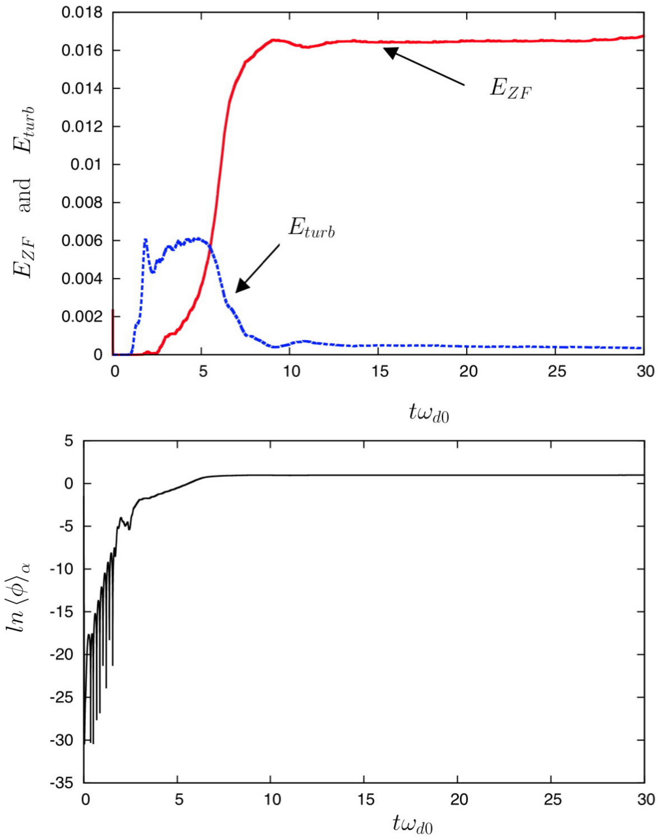
Figure 3.
Time evolution of (shown with the dotted and blue line) in the kinetic regime of zonal flow (ZF), in the top panel. In the bottom panel, the time evolution of the squared mean potential in a logarithmic scale. There is a qualitative change in the interchange turbulence, which exhibits a weaker simultaneous growth of and until saturation, at time , and an oscillatory behavior of at low frequency. Here, the physical parameter is The corresponding evolution of the zonal flow component is taken at (in unit).
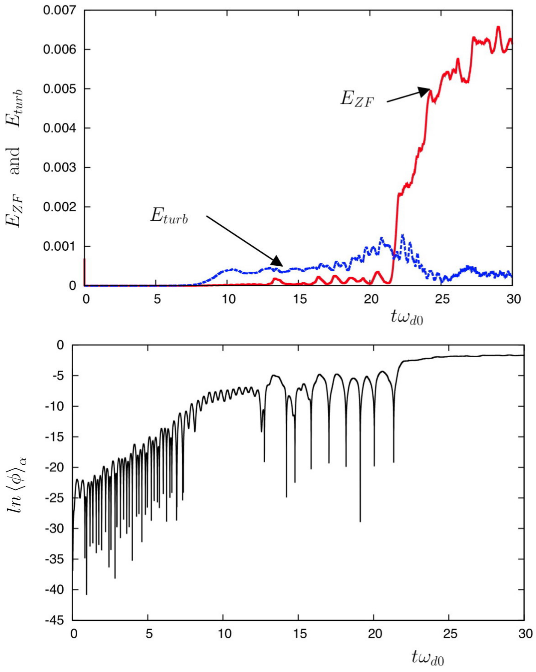
Figure 4.
On the top panel: temporal evolution of the quantities (in red and in solid line) and of the turbulent component (now in blue and in dotted line) for for a long time. On the bottom panel: the corresponding time evolution of the mean electric potential in a logarithmic scale. The zonal flow energy displays three different stages during its evolution: a first phase characterized by a weak growth-rate for time , followed by a first resonant peak at and finally a second resonant process, now located at time , followed by a slow reduction of the turbulence. The plot of was taken at (in unit).
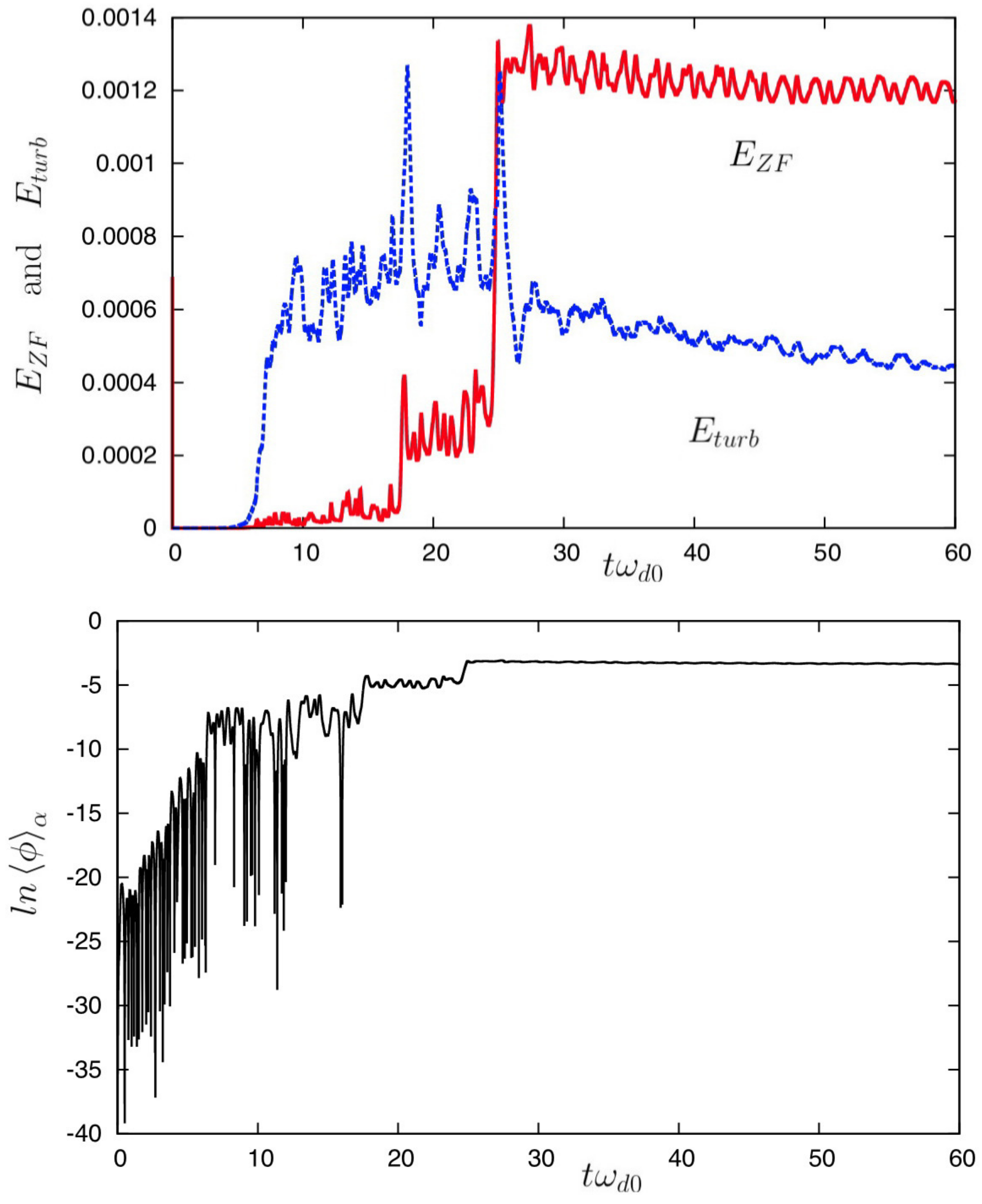
Figure 5.
Continuing the presentation of results of the simulation shown in Figure 4, the spectrum in frequency of the electric potential is shown. We observe clearly both components of zonal flow (ZF), the quasi-zero part driven by the Reynolds tensor (fluid regime) and the low-frequency zonal flow (LFZF) component (in the kinetic regime), at a frequency close to .
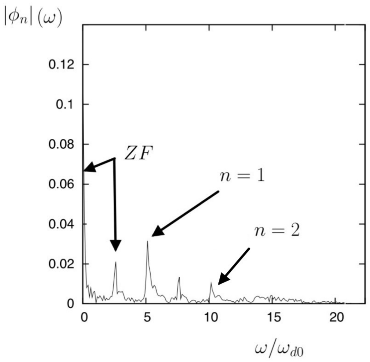
Figure 6.
Continuing the results of simulation shown in Figure 4 and Figure 5, the electric potential is plotted at three different times when the resonance takes place, showing clearly that the dominant modes are and in the asymptotic regime. We have identified a nonlinear coupling of zonal flow (ZF) mediated by nonlinear collisionless trapped ion modes (TIMs), leading to a strong reduction of the interchange turbulence.
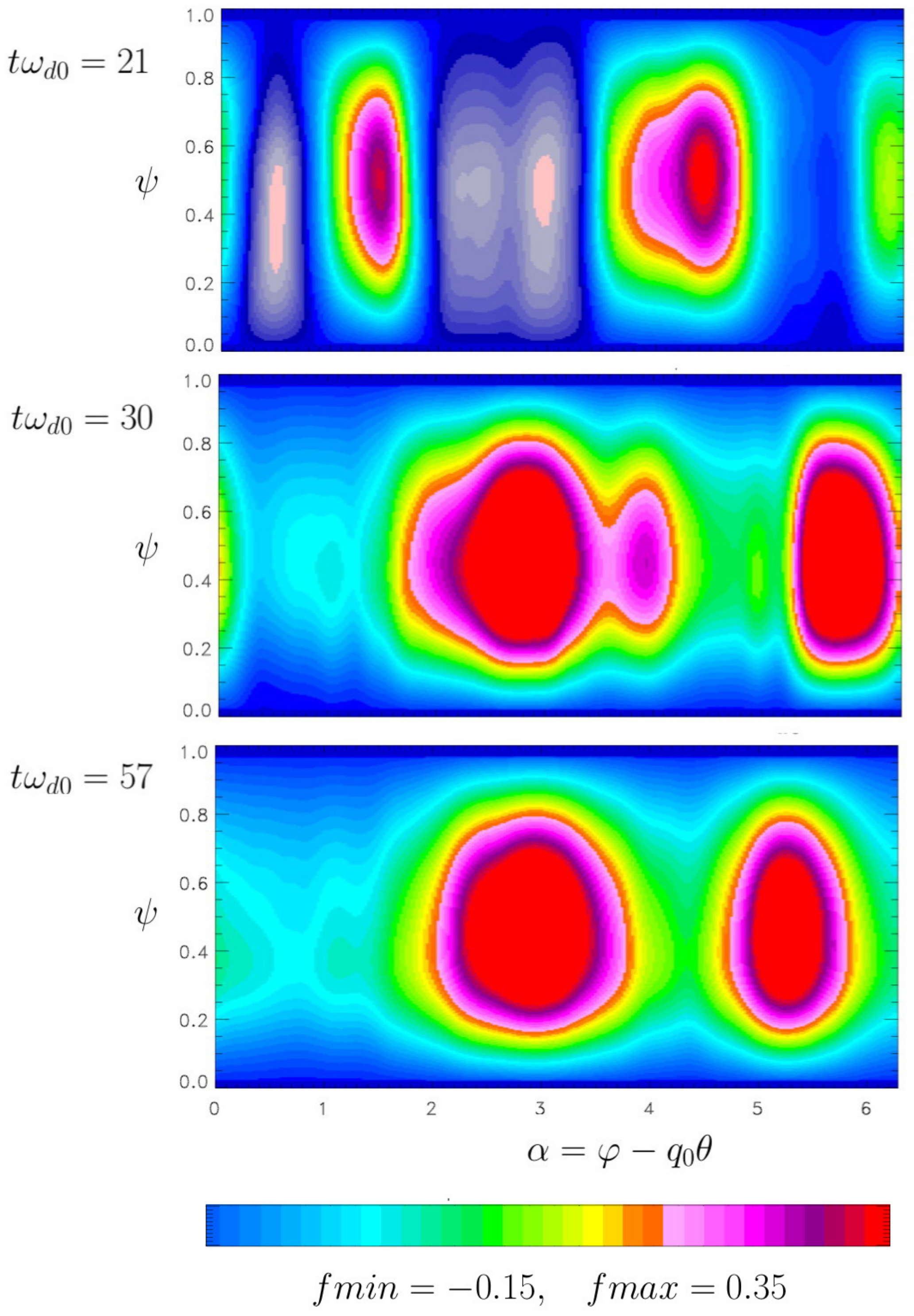
Figure 7.
Continuing the results of simulation shown previously in Figure 4, Figure 5 and Figure 6, we have plotted the mean ion pressure , displayed on the left panel, as a function of the poloidal flux and the corresponding electric potential representation on the right panel, showing the formation of a transport-barrier region (located around .
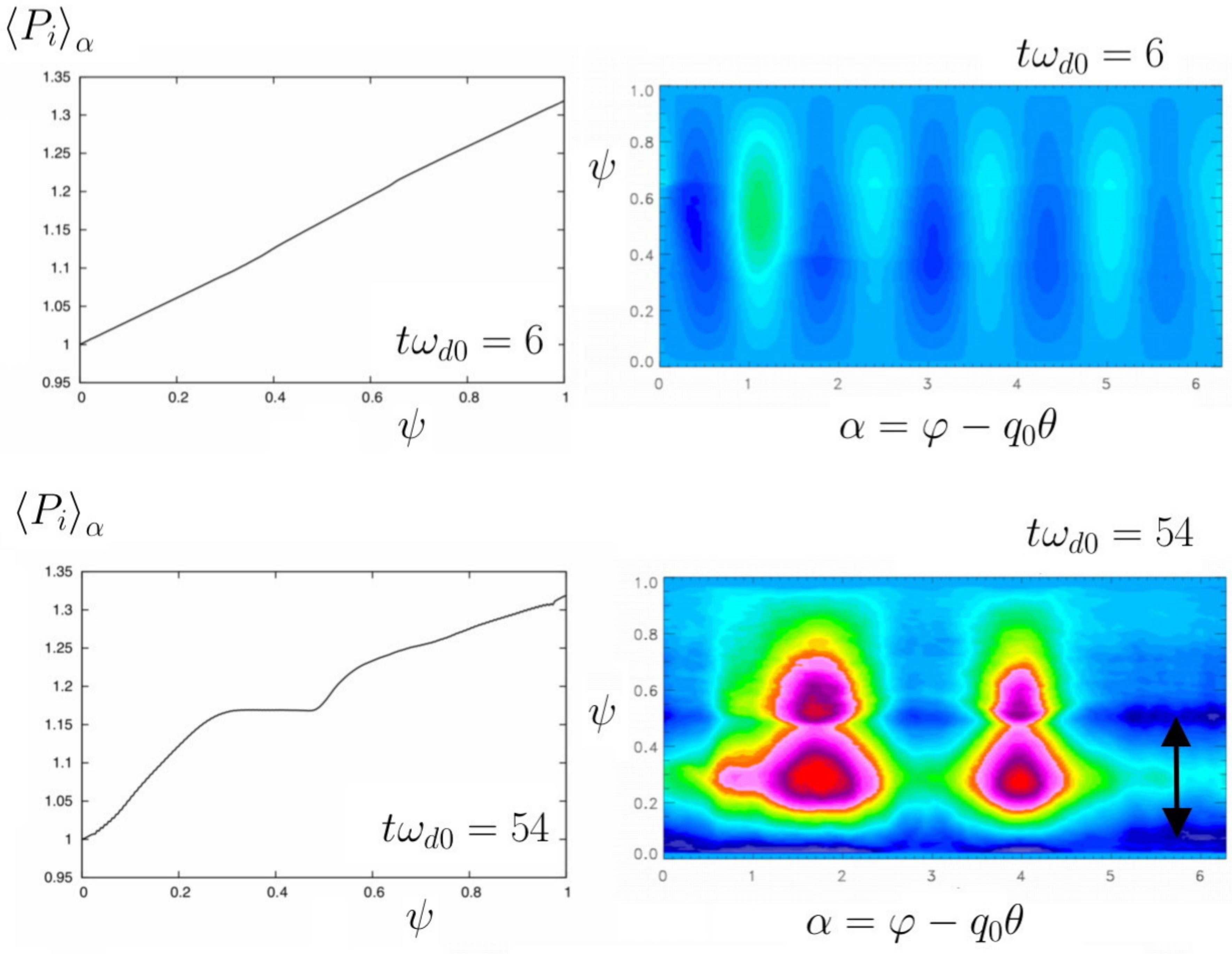
Figure 8.
Plot of the turbulent energy (shown in the dotted and blue line) in the kinetic regime. In the bottom panel, the time evolution of the squared mean potential in a logarithmic scale. There is a qualitative change in the interchange turbulence, which exhibits a weaker simultaneous growth of and until saturation, at time , and an oscillatory behavior of at low frequency. Here, the physical parameter is In the saturation phase of the instability, zonal flow (ZF) features linear trapped ion modes (TIMs) (with a frequency with no frequency shift. The plot of was taken at (in unit).
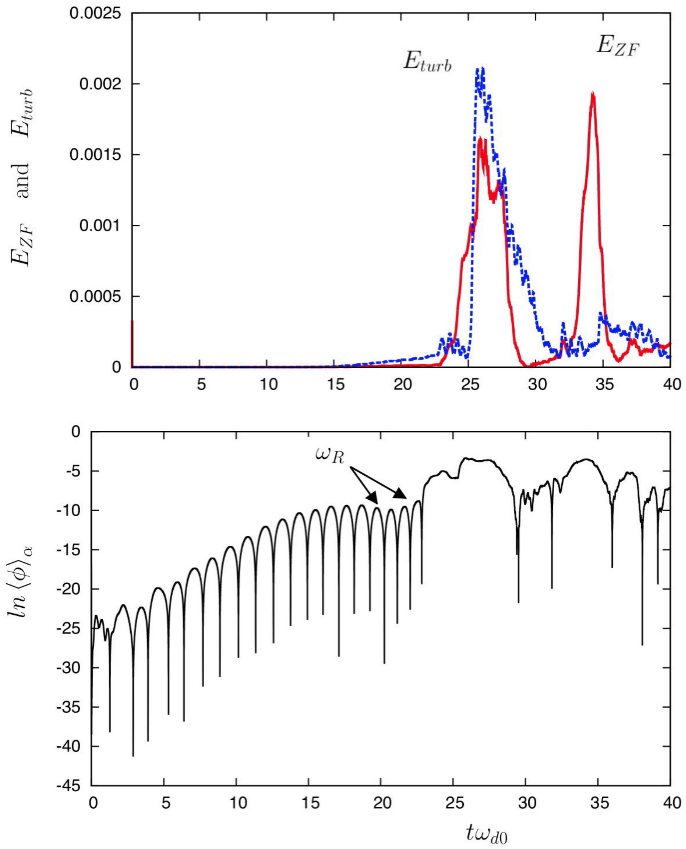
Figure 9.
Diagrams show that streamers are also occurring but on a higher mode (with a toroidal number of as can be seen on the plot shown at time . Here, the polarization factor is
Figure 9.
Diagrams show that streamers are also occurring but on a higher mode (with a toroidal number of as can be seen on the plot shown at time . Here, the polarization factor is
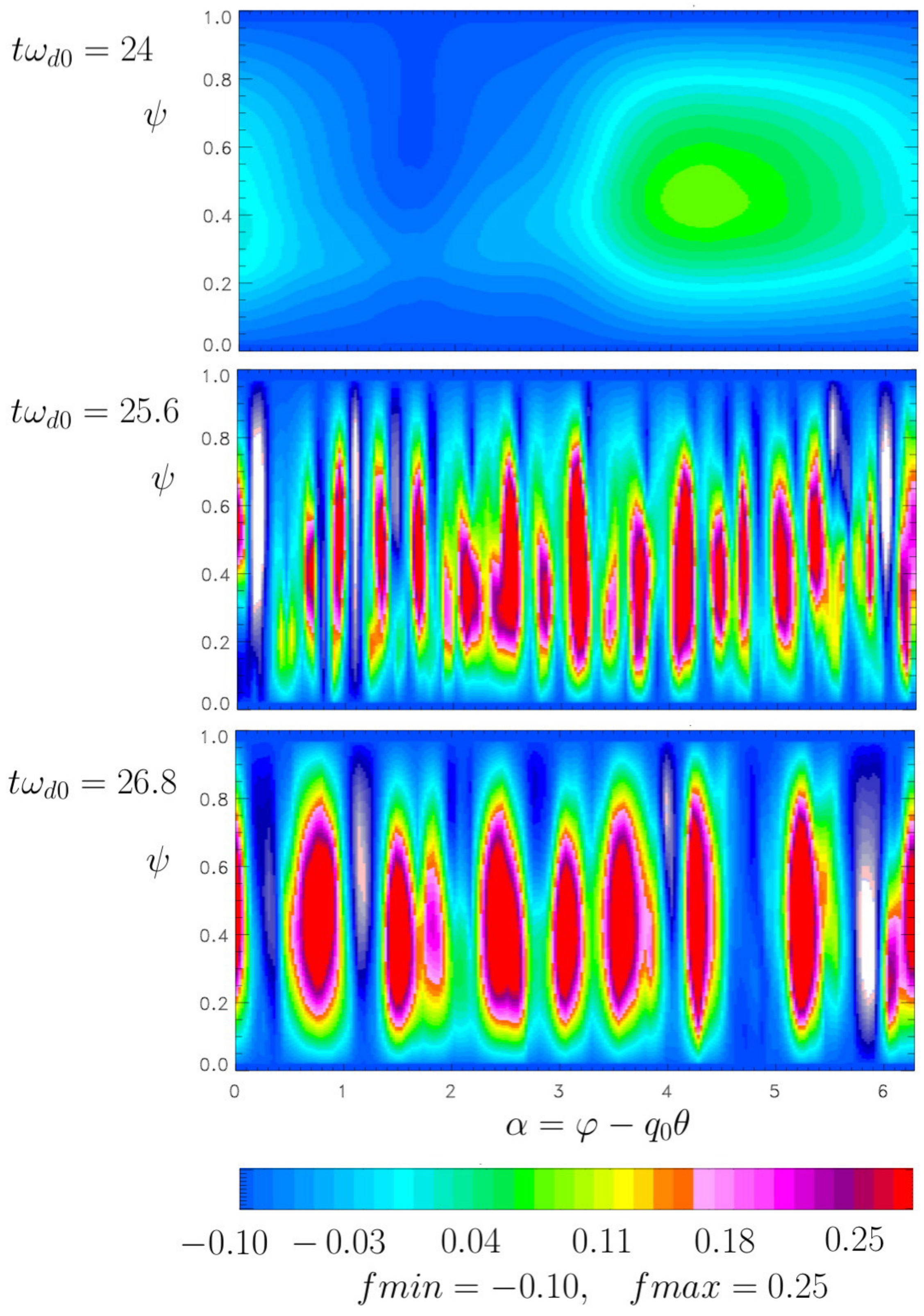
Figure 10.
Spectra in wave-numbers, i.e., in toroidal numbers. The spectra reveal the occurrence of (nonlinear) streamers with a broad spectrum (with a toroidal number of n∼16–24) as can be seen on the plot shown at time .
Figure 10.
Spectra in wave-numbers, i.e., in toroidal numbers. The spectra reveal the occurrence of (nonlinear) streamers with a broad spectrum (with a toroidal number of n∼16–24) as can be seen on the plot shown at time .

Figure 11.
Basic mesoscale structures met in tokamak device (streamer and zonal flow) at left. The right side illustrates the corresponding mesoscale structures (zonons and zonal jets) found in the atmosphere. In the 2D description of drift-kinetic turbulence in a tokamak, the restriction to a planar geometry corresponds to the condition, which holds for both zonal flows and streamers. In the 2D description of zonostrophic turbulence, the restriction to a 2D geometry is given instead by the condition . The correspondence between the set of toroidal coordinates in drift-kinetic turbulence in tokamaks and the set of spherical coordinates in zonostrophic turbulence in the atmosphere is shown here.

Table 1.
Summary of different types of waves and coupling processes in both interchange-type turbulence and zonostrophic turbulence.
Table 1.
Summary of different types of waves and coupling processes in both interchange-type turbulence and zonostrophic turbulence.
| Turbulence | Zonostrophic | Interchange (CTIM) |
|---|---|---|
| potential vorticity | ||
| linear waves | Rossby-Haurwitz | trapped ion mode (TIM) |
| frequency | ||
| nonlinear waves | zonons | streamers |
| inhomogeneity | -effects | |
| zonal flow | jets, zonal band | electrostatic zonal flow (ZF) |
| low-frequency zonal flow (LFZF) | ||
| amplification | by resonant triad | by resonant triad |
| role of zonal flow (ZF) | transport barriers | transport barriers |
© 2017 by the authors. Licensee MDPI, Basel, Switzerland. This article is an open access article distributed under the terms and conditions of the Creative Commons Attribution (CC BY) license (http://creativecommons.org/licenses/by/4.0/).
Share and Cite
MDPI and ACS Style
Sarto, D.D.; Ghizzo, A. Hasegawa–Wakatani and Modified Hasegawa–Wakatani Turbulence Induced by Ion-Temperature-Gradient Instabilities. Fluids 2017, 2, 65. https://doi.org/10.3390/fluids2040065
AMA Style
Sarto DD, Ghizzo A. Hasegawa–Wakatani and Modified Hasegawa–Wakatani Turbulence Induced by Ion-Temperature-Gradient Instabilities. Fluids. 2017; 2(4):65. https://doi.org/10.3390/fluids2040065
Chicago/Turabian StyleSarto, Daniele Del, and Alain Ghizzo. 2017. "Hasegawa–Wakatani and Modified Hasegawa–Wakatani Turbulence Induced by Ion-Temperature-Gradient Instabilities" Fluids 2, no. 4: 65. https://doi.org/10.3390/fluids2040065