Effect of the Non-Stationarity of Rainfall Events on the Design of Hydraulic Structures for Runoff Management and Its Applications to a Case Study at Gordo Creek Watershed in Cartagena de Indias, Colombia

Abstract

The 24-h maximum rainfall (P_24h-max) observations recorded at the synoptic weather station of Rafael Núñez airport (Cartagena de Indias, Colombia) were analyzed, and a linear increasing trend over time was identified. It was also noticed that the occurrence of the rainfall value (over the years of record) for a return period of 10 years under stationary conditions (148.1 mm) increased, which evidences a change in rainfall patterns. In these cases, the typical stationary frequency analysis is unable to capture such a change. So, in order to further evaluate rainfall observations, frequency analyses of P_24h-max for stationary and non-stationary conditions were carried out (by using the generalized extreme value distribution). The goodness-of-fit test of Akaike Information Criterion (AIC), with values of 753.3721 and 747.5103 for stationary and non-stationary conditions respectively, showed that the latter best depicts the increasing rainfall pattern. Values of rainfall were later estimated for different return periods (2, 5, 10, 25, 50, and 100 years) to quantify the increase (non-stationary versus stationary condition), which ranged 6% to 12% for return periods from 5 years to 100 years, and 44% for a 2-year return period. The effect of these findings were tested in the Gordo creek watershed by first calculating the resulting direct surface runoff (DSR) for various return periods, and then modeling the hydraulic behavior of the downstream area (composed of a 178.5-m creek’s reach and an existing box-culvert located at the watershed outlet) that undergoes flooding events every year. The resulting DSR increase oscillated between 8% and 19% for return periods from 5 to 100 years, and 77% for a 2-year return period when the non-stationary and stationary scenarios were compared. The results of this study shed light upon to the precautions that designers should take when selecting a design, based upon rainfall observed, as it may result in an underestimation of both the direct surface runoff and the size of the hydraulic structures for runoff and flood management throughout the city.

1. Introduction

Climate change is gradually coming to affect all living species by giving rise to new sets of meteorological conditions: record breaking high temperatures, melting glaciers, increasing sea water levels, increasing severity of droughts, floods, tornadoes, and hurricanes, to mention just a few. Hydraulic structures have not been the exception; most of these structures were designed was based on rainfall patterns that, in some cases, no longer conform to the realities of today’s weather conditions. Generally speaking, sizing a hydraulic structure for an ungauged watershed starts with a hydrological analysis that includes: (a) a rainfall frequency analysis; (b) the watershed delineation and estimation of its morphometric parameters; and (c) the direct surface runoff (DSR) calculation using a rainfall-runoff model, assuming it has the same return period of the generating rainfall.

Usually, a rainfall frequency analysis for an ungauged watershed consists of trying to find the probability distribution that best represents the behavior of the extreme events (of different durations) being analyzed, in order to subsequently obtain the value of the precipitation event associated with a given return period to be later used for the DSR estimation. The traditional methods for frequency analysis of extreme values for hydraulic structures design (streamflow, rainfall or rainfall intensity) assume that: (a) the values of the variable are random and independent; (b) the probability distribution functions are stationary; and (c) the return period (Tr) is the inverse of the probability of exceedance (p). These assumptions imply that the probability of an event producing excessive precipitations does not change over time (the sample is homogeneous). This approach cannot be applied when the variable being analyzed shows noticeable change of pattern (either increase or decline), which may indicate non-stationary conditions [1,2,3,4]. In these cases, the typical definition of the return period (Tr = 1/p) has to be redefined to account for non-stationarity.

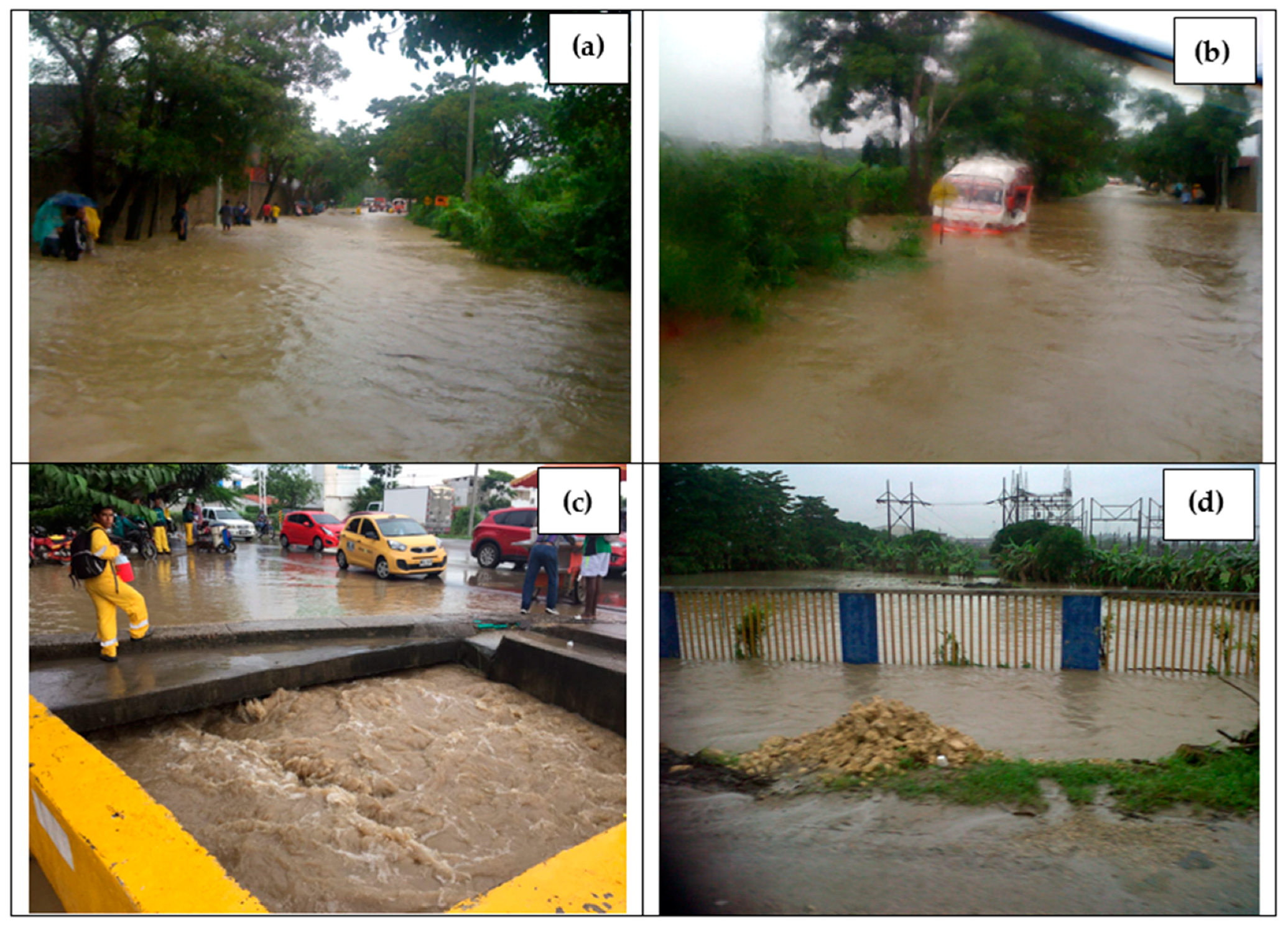
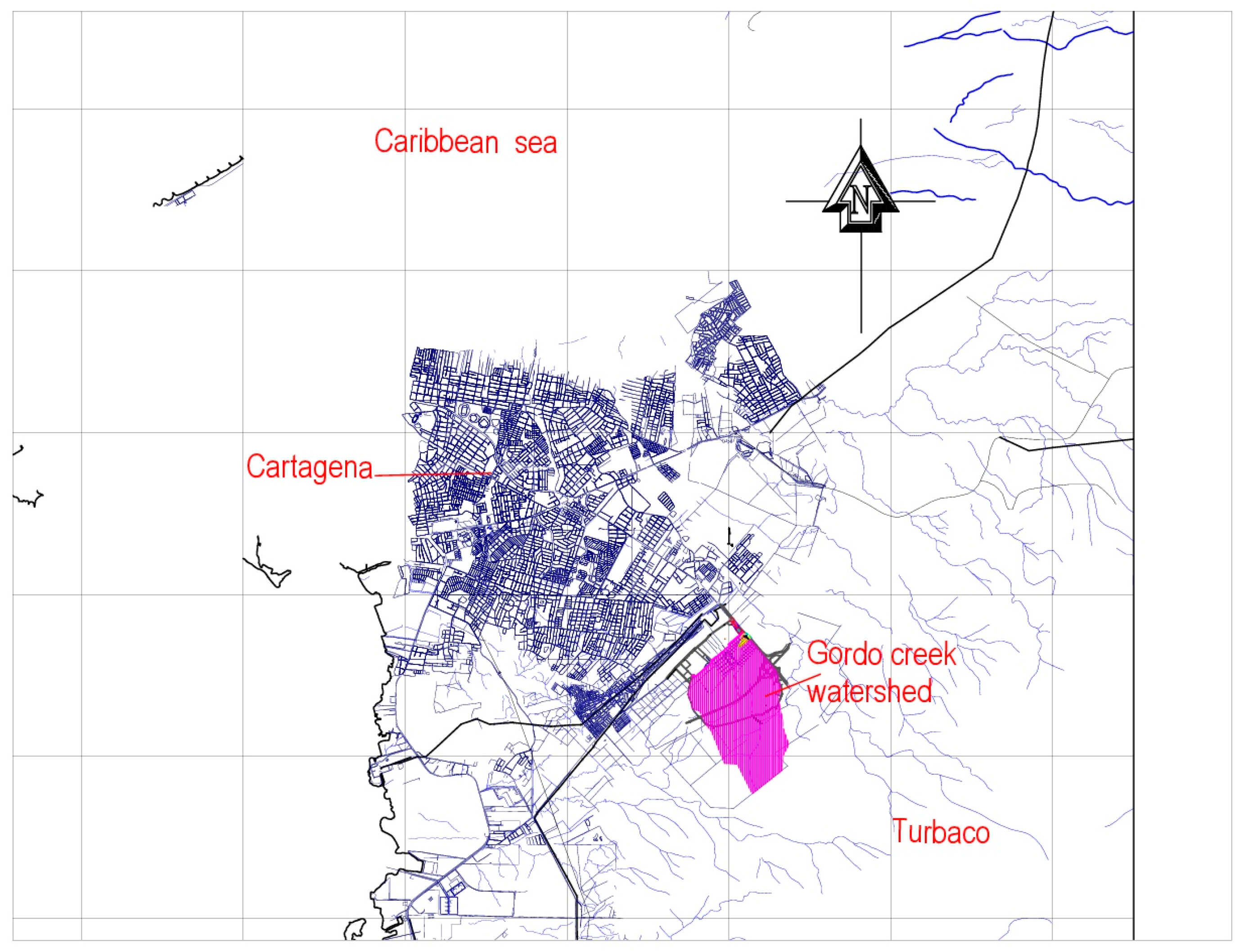
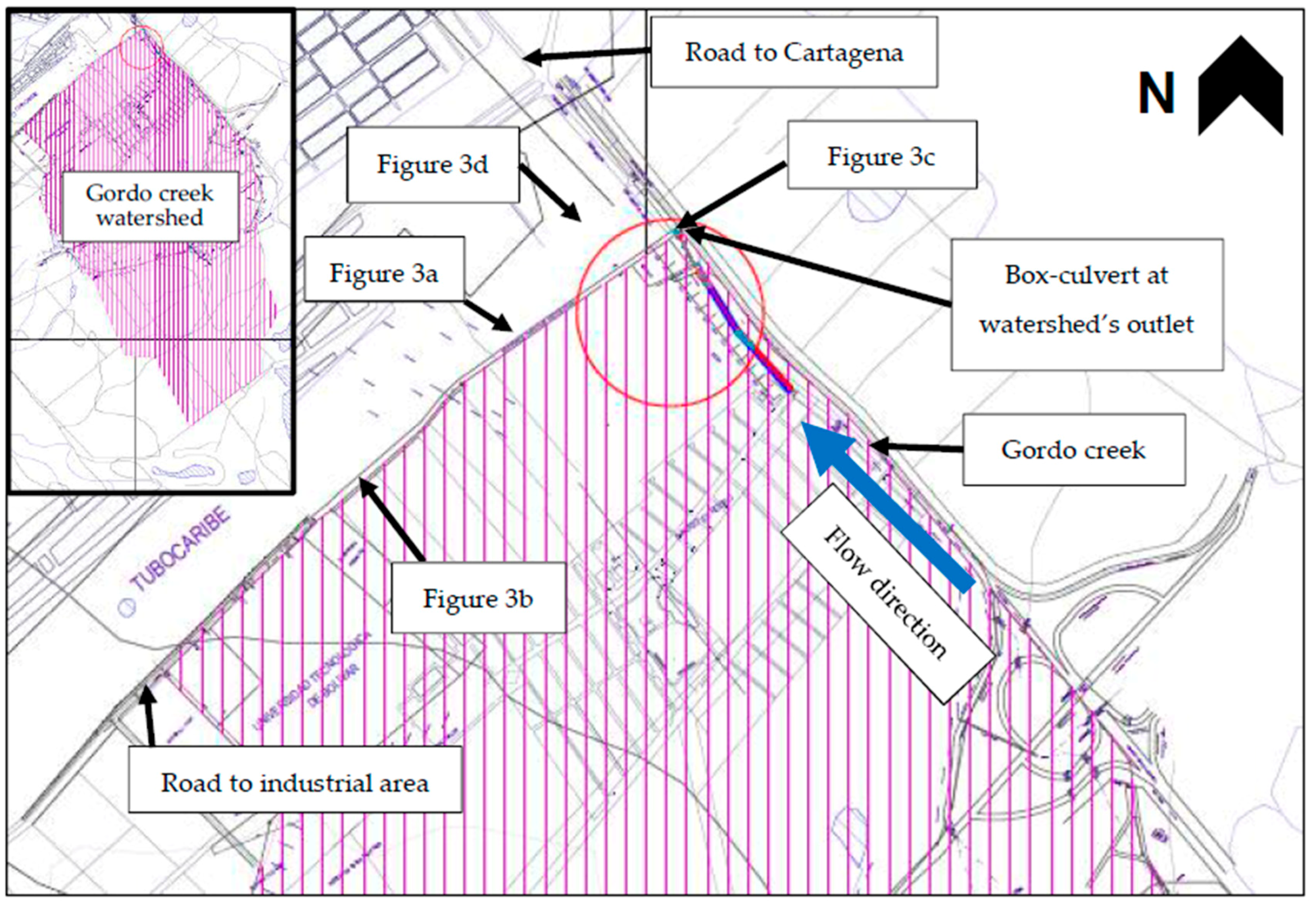
Cartagena de Indias, a city on the Caribbean coast of Colombia, has been lately undergoing recurring floods that can be mainly attributed to different factors that go from uncontrolled development projects—due to the lack of an updated territorial management plan that fits the city’s realities—to poorly designed hydraulic structures for runoff management that do not take future conditions (especially rainfall pattern changes and increase of impervious areas) into account. Most of the runoff of Cartagena de Indias discharges into La Virgen swamp (ciénaga de La Virgen), a waterbody of approximately 502 km², whose southern shoreline has been populated over the years by illegal low-income settlements that suffer the consequences of both a rising sea level (the swamp is connected to the Caribbean Sea) and an obsolete stromwater system. Furthermore, the cities of Cartagena de Indias (downstream) and Turbaco (upstream) share several watersheds that also drain into the La Virgen swamp. The upstream areas of these watersheds (like the one selected in this study) are mostly rural, which have been gradually converted into impervious areas by local developers that offer more competitive prices than those in Cartagena de Indias. This dynamic will most likely (and rapidly) change the landscape, which brings with it more challenging hydrologic, and hydraulic, conditions.

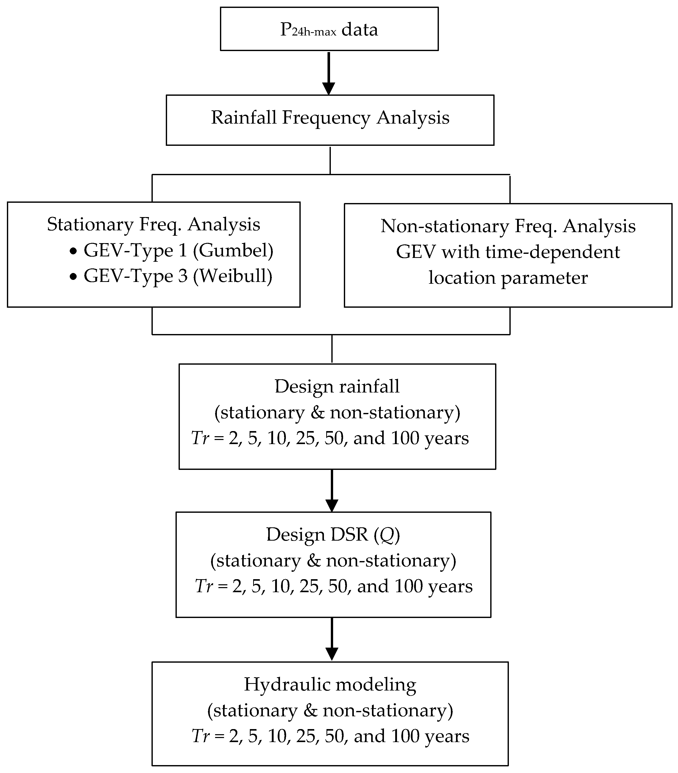
In this context, Colombian legislation has mandated to analyze the possible effects of climate change on the future rainfall pattern if a stormwater system (channels, pipes, culverts, etc.) is to be designed [5]. A regional increasing trend of both rainfall and streamflow has been found in some areas of the northern portion of the Colombian Caribbean region [6,7]. The studies that carry out assessments for stationary (SC) versus non-stationary (NSC) conditions of streamflow and/or rainfall, typically encompass only performing a statistical analysis (of a trend) without quantifying how the two scenarios may affect real life conditions, both hydrologically and hydraulically speaking. In this study, multiannual 24-h maximum rainfall (P_24h-max) data (from the synoptic weather station located at the Rafael Núñez airport) was used to: (a) assess the trend of the P_24h-max observations over time, specifically for Cartagena de Indias, (b) quantify the rainfall values obtained for several return periods (2, 5, 10, 25, 50, and 100 years) via stationary and non-stationary frequency analyses, (c) carry out a hydrological and hydraulic analysis on the Gordo creek watershed under SC and NSC for different return periods in order to understand the recurring floods reported that affect a commercial and industrial area downstream, and (d) point out the importance of accounting for the effect of climate change in the decision making process in runoff management, especially in flood-prone areas.

2. Study Area and Data

2.1. Study Area

The Gordo creek watershed is located within the jurisdiction of the city of Turbaco (Colombia); the outlet is at the east-southern borderline between the cities of Cartagena de Indias and Turbaco (Figure 1). It has a total area of 258 hectares. The creek runs south to north, with a total length of 2962 m and an average slope of 0.00454. The watershed’s centroid and outlet are located at the geographical coordinates 10°20′04′′ N; 75°27′29′′ W and 10°22′34.83′′ N; 75°27′37.51′′ W respectively.

The watershed’s soil cover in the upstream area is mostly rural (bush and forest) while the downstream is in a busy commercial, industrial, and residential area (

Table 1. Gordo creek watershed’s soil cover distribution.

Item	Developed Areas			Rural Areas		Total
	Impervious	Urban	Residential	Bush	Forest
Area (ha)	2.9	12.7	23.4	109.5	109.5	258

). The soil texture is predominantly clay-loam with a poor infiltration capacity when saturated.

The watershed’s downstream area has a main road with a box-culvert that gives access to several industries and businesses. The most critical portion of the watershed’s downstream area (circled area in Figure 2) is composed of the last 178.5-m reach (of the creek) and the box-culvert that controls the watershed outlet. Flooding events occur every year during the rainy season (September through November), which impedes regular transit for several hours. Also, people and vehicles have been stranded, and have required rescuing on the flooded road (Figure 3a–d).

2.2. Rainfall Data

Although the Institute of Hydrology, Meteorology, and Environmental Studies of Colombia (IDEAM, in Spanish) operates another two weather stations in Cartagena de Indias (Escuela Naval-CIOH and Santa Ana), the one located at the airport Rafael Núñez has the longest and most complete data of records for several meteorological variables (

Table 2. Description of Rafael Núñez airport weather station.

Station	Type	IDEAM ID N°	Height (masl)	Geographic Coord.		Operating Period
				North	West	Start	Finish
Rafael Núñez Airport	Synoptic (*)	14015020	2	10°26′31′′	75°31′13′′	15 March 1941	Still active

(*) Meteorological variables measured hourly (synoptic time) at a synoptic weather station include: precipitation, cloud conditions, wind direction and velocity, atmospheric pressure, air temperature, visibility, and humidity. Precipitation at Rafael Núñez station is measured by means of a Hellmann-Fuess pluviograph (standard model; rain recorder 95).

); for this reason, it is the most used in hydrological and hydraulic analysis and designs.

For this study, continuous multiannual observations of 24-h maximum rainfall (P_24h-max) from 1941 to 2015 (

Table 3. Multiannual P_24h-max observations of Rafael Núñez airport (1941–2015).

Year	1941	1942	1943	1944	1945	1946	1947	1948	1949	1950	1951
P24h-max (mm)	60.0	35.0	30.0	89.0	71.0	60.0	60.0	107.0	54.0	85.0	93.0
Year	1952	1953	1954	1955	1956	1957	1958	1959	1960	1961	1962
P24h-max (mm)	41.0	51.0	90.0	110.0	95.0	40.0	109.0	68.0	109.0	65.0	75.0
Year	1963	1964	1965	1966	1967	1968	1969	1970	1971	1972	1973
P24h-max (mm)	59.0	69.0	89.0	76.0	67.0	89.0	129.0	157.0	104.7	120.0	74.1
Year	1974	1975	1976	1977	1978	1979	1980	1981	1982	1983	1984
P24h-max (mm)	126.4	101.6	54.4	60.5	68.6	120.7	135.9	124.4	98.0	63.4	102.7
Year	1985	1986	1987	1988	1989	1990	1991	1992	1993	1994	1995
P24h-max (mm)	164.5	64.9	171.3	115.0	201.8	77.8	32.5	161.5	133.4	54.8	76.3
Year	1996	1997	1998	1999	2000	2001	2002	2003	2004	2005	2006
P24h-max (mm)	99.4	99.6	85.6	108.5	116.2	76.2	73.5	161.8	149.0	76.4	122.3
Year	2007	2008	2009	2010	2011	2012	2013	2014	2015	-	-
P24h-max (mm)	183.1	95.3	61.3	150.7	146.1	94.2	88.0	116.0	51.8	-	-

; gray cell is the maximum value registered) were used. Years 2016 and 2017 have not yet been officially reported by IDEAM.

3. Methodology

The methodology used in this research is presented in the flowchart of Figure 4. Each step is described in detail in the following sub-sections.

3.1. Rainfall Stationary Frequency Analysis

The stationary frequency analysis is based on the following assumptions: (a) the cumulative distribution functions (CDFs) do not change over time [2] and (b) the variable analyzed must be random and independent [1]. In hydrology, there are several CDFs for the analysis of extreme values, namely: gamma, extreme value (EV) or Fisher-Tippett (types 1, 2, and 3), generalized extreme value (GEV), log-normal, Pearson 3, Log-Pearson 3, among others. The GEV was used for the frequency analysis carried out in this section, as it has shown to work best in Colombia.

The expression for the GEV distribution is given by Equation (1), where F(Z) is the CDF, z is the random variable, k is the shape (or shift) parameter, β is the mode (location parameter), and α is the dispersion (scale parameter). The GEV distribution may adopt one of the three types of the EV distribution depending upon the value of k [8,9,10]: (a) when k equals zero, EV is type 1 (Gumbel) [11]; (b) when k is less than zero, EV is type 2 (Frechet) [12]; and (c) when k is greater than zero, EV is type 3 (Weibull) [13].

$$F\left(Z\right)= \exp \left[-{\left(1-k\frac{z-\beta }{\alpha }\right)}^{1/k}\right]$$

(1)

The estimated GEV’s parameters were: α = 31.35 mm, β = 78.097 mm, and k = 0.06.

Table 4. P_24h-max values for stationary freq. analysis.

Tr (year)	P24h-max
	Gumbel	Weibull
2	88.6	89.2
5	124.4	125.0
10	148.1	148.1
25	178.1	176.4
50	200.3	196.9
100	222.4	216.8

Bold values indicate the largest value of the two CDF used.

shows the values of the P_24h-max for each of the two methods used. Gray cells show maximum values.

Lastly, the CDF goodness-of-fit was carried out via Chi-square [13] and Kolmogorov-Smirnov [14,15,16,17] tests. Values of 0.06001 and 2.2876 were obtained for the Kolmogorov-Smirnov and Chi-square tests respectively. These results indicate that the GEV distribution accurately represents the behavior of the rainfall data analyzed.

3.2. Rainfall Non-Stationary Frequency Analysis

The non-stationary analysis considers the following assumptions [2,3,4]: (a) the probability of exceeding the random variable over the years (p_j) of the CDFs may increase or decrease, and (b) the extreme values of the analyzed variable are independent in time. Parameters of the CDFs are considered time-varying in order to compute the probability of exceeding occurring, which implies that extreme values are not identically distributed over time.

To define the return period under non-stationary environments (Tr,_NSC), it is necessary to understand the concept of the waiting time. The waiting time is a random variable (X) defined as the occurrence of a value exceeding the design value for the first time. In stationary conditions, the probability of exceeding remains constant over time, which implies that a geometric distribution can be used to compute the expected value (E(x) = Tr, SC = 1/p). Commonly, this is called the return period [8]. In contrast, under non-stationary conditions, the return period (Tr) is computed with a non-homogeneous geometric distribution (Equation (2)) [18]:

$$Tr{,}_{NSC}=1+{\displaystyle \sum }_{x=1}^{\infty }{\displaystyle \prod }_{j=1}^x\left(1-p_j\right)$$

(2)

where p_j is the time-varying probability of exceeding, and the subscript j represents the projecting year.

The GEV distribution with a temporal trend in the location parameter (β_t) can be expressed as (Equation (3)) [2,18]:

$$F\left(Z,{\beta }_t\right)= \exp \left[-{\left\{1+k\left(\frac{z-{\beta }_t}{\alpha }\right)\right\}}^{-1/k}\right]$$

(3)

The P_24h-max data at the Rafael Núñez airport weather station (Table 4) exhibits an increasing linear trend over time (dotted black line in Figure 5), which confirms the non-stationary occurrence of the analyzed variable.

To estimate the P_24h-max values, the non-stationary frequency analysis followed these steps [4,18]: (a) selecting the CDF under non-stationary condition (GEV or Gumbel); (b) defining a model (constant, linear, or establishing other models) of each parameter (location, shape, and scale) with its trend (increasing or decreasing); (c) estimating parameters by likelihood method; (d) calculating the goodness-of-fit test of the Akaike Information Criterion (AIC) [19] and then selecting the CFD with the minimum value of it; and (e) estimating the P_24h-max for various return periods.

For this study, the CDF under non-stationary condition (GEV distribution) was selected considering the distribution used in the stationary scenario of Section 3.1. The GEV’s parameters were estimated by means of a code [2,18] programmed in R software (version 3.3.1, R Development Core Team, Auckland, New Zealand) with the library nsextremes. The resulting linear trend lines for the location (increasing trend) and scale (remains constant) parameters are shown in Figure 5 (blue and green lines for the location and scale parameters, respectively). The values of the aforementioned parameters were: βt = 79.543 mm + [(0.4949 mm/year) (t_mean – 1978)], α = 31.1 mm, and k = −0.106. The t_mean term in the previous expression represents an analyzed year centered over its own mean between 1941 and 2015. A sensitivity analysis showed that variations of both the scale and the shape parameters do not bring an adequate trend for the P_24h-max when the results were compared with the findings of IDEAM. The AIC test was used in order to evaluate the GEV distribution goodness-of-fit by comparing both scenarios (stationary and non-stationary). The obtained values were 747.5103 (non-stationary) and 753.3721 (stationary). The results of the P_24h-max for several return periods are presented in

Table 5. P_24h-max values for non-stationary freq. analysis.

Tr (year)	P24h-max (mm)
2	128.1
5	140.6
10	161.5
25	189.1
50	213.1
100	244.8

.

3.3. Curve Number (CN) Estimation

Given that the Gordo creek watershed is composed of several soil cover types, an area-based composite CN was estimated following the methodology established in the National Engineering Handbook, Section 4 (NEH-4) [20], where a series of lookup tables are given for different combinations of hydrological soil groups (HSGs) and soil cover. The HSG of the watershed is C, as per the description of the soil texture provided in Section 2.1 (clay-loam soil texture). The values shown in those tables represent what is called the average antecedent runoff condition (ARC-II). The ARC is a concept introduced into the CN methodology to try to account for the potential for runoff generation in a watershed due to the soil water content after several rainfall events [21]. For that, the total amount of cumulative rainfall of the 5 previous days (5-day antecedent precipitation, P₅) is estimated to establish whether the soil is in dry, average/normal or wet (

Table 6. ARC types based on P₅.

ARC Type	Dormant Season	Growing Season
I (dry)	<12.7 mm	<36 mm
II (normal)	12.7–27.9 mm	36–53 mm
III (wet)	>27.9 mm	>53 mm

) [21]; a set of equations are then proposed to adjust the CN accordingly (Equations (4) and (5)) [8,22].

$${\mathrm{CN}}_{\mathrm{I}}=\frac{{\mathrm{CN}}_{\mathrm{II}}}{2.281-0.01281{\mathrm{CN}}_{\mathrm{II}}}$$

(4)

$${\mathrm{CN}}_{\mathrm{III}}=\frac{{\mathrm{CN}}_{\mathrm{II}}}{0.427-0.00573{\mathrm{CN}}_{\mathrm{II}}}$$

(5)

In 2010–2011, Colombia underwent the longest and most devastating rainy season ever recorded. Floods were reported throughout the country, especially in the Caribbean coastal region. In this study, a CN adjustment was carried out for ARC_III to mimic a saturated soil as the most critical scenario in the Gordo creek watershed in that season, during which more than 53 mm of rain fell in 5 consecutive days.

Table 7. Composite CN for Gordo creek watershed.

Item	CN Developed Areas			CN Rural Areas
	Impervious	Urban	Residential	Bush	Forest
CNII	98	88	85	86	60
CNIII	99.1	94.4	92.9	93.4	77.5
Area (ha)	2.9	12.7	23.4	109.5	109.5
CNII sub-areas	86.9			73
CNII composite	75.1
CNIII sub-areas	93.8			85.5
CNIII composite	86.7

shows the values of CN composite obtained for average and wet conditions (gray cells).

3.4. Time of Concentration Estimation

The time of concentration may be defined as the time it takes a drop of water to travel from the hydraulically most remote point to the watershed outlet (or any other point of interest) [23]. It is one of the most critical parameters for any hydrological analysis and the subsequent design of a hydraulic structure aimed at managing stormwater. Many methodologies (empirical and semi-empirical) have been proposed for its estimation [24,25]. For this study, the Kirpich method was used (Equation (6)) [26], as the Gordo creek watershed fits some of the morphometric characteristics needed for using this formula [25].

$$Tc=0.0195L^{0.77}{S}^{-0.385}$$

(6)

In Equation (6), Tc is the time of concentration (min), L is the length of the main watercourse/channel (m) and S is the average slope of the main watercourse/channel (m/m). After plugging the L and S values provided in Section 2.1, the Tc equals 73.3 min.

3.5. Direct Surface Runoff (DSR) Estimation

The DSRs produced by the rainfall under both stationary and non-stationary conditions for different return periods (2, 5, 10, 25, 50, and 100 years) were estimated (

Table 8. Peak flow values.

Tr (year)	Peak Flow (m3/s)
	SC	NSC
2	14.3	25.3
5	24.3	29.0
10	31.2	35.2
25	40.2	43.6
50	47.1	51.0
100	53.9	60.9

) via Hydrologic Engineering Center Hydrologic Modeling System (HEC-HMS), which is a CN-based hydrological model developed by the U.S. Corps Army of Engineers [27]. HEC-HMS compiles several methodologies for hydrological analysis integrated into one tool capable of quickly modeling different scenarios at the same time.

Apart from the adjusted CN value estimated in Section 3.3, the HEC-HMS simulations for the various return periods were made under the following conditions: (a) 3-h rainfall as it is the most typical duration historically observed in Cartagena de Indias; (b) the 3-h rainfall corresponds to 79% of the P_24h-max, and its distribution was estimated via multiannual probabilistic analysis of 30 pluviographs [8] (Figure 6) (P90% was the one used; it indicates the probability that the rainfall pattern observed falls to the left of the P90% curve); (c) no rainfall area reduction was needed due to the size of the watershed; (d) hydrograph generation via SCS-unit hydrograph method; and (e) a lag time of 0.6 Tc (Tlag = 0.6Tc). Table 8 summarizes the peak flow values for stationary and non-stationary conditions.

3.6. Channel Hydraulic Modeling

A one-dimension (1-D) hydraulic modeling was carried out using the Hydrologic Engineering Center River Analysis System (HEC-RAS) software, developed by the U.S. Corps Army of Engineers. The simulation was performed under gradually varied flow and subcritical conditions (Froude number less than 1). Also, the following inputs were utilized in the simulation: (a) Gordo creek’s bathymetry, that includes ten cross-sections (Figure 7) of the last 178.5 m of the stream (the most critical portion of the watershed) which consist of a natural cross-section with three culverts; (b) design DSR for several return periods estimated in Section 3.5; (c) hydraulic control section governed by a subcritical flow at the downstream box culvert (section K0+000), which produces a backwater profile in the entire channel. The natural channel exhibits different cross-sections, as presented in Figure 8a,b.

Figure 9a,b show the plant view and the longitudinal profile of Gordo creek watershed outlet (gray-shaded areas show the location of culverts). A description of the culverts is presented in

Table 9. Description of culverts.

Channel		Section			Slope (%)
From	To	Type	Number of Cells	Dimensions
K0+000	K0+008.44	Box culvert	2	2.5 m × 2.0 m	1.25
K0+012.44	K0+062.44	Pipe culvert	2	Diameter of 1.6 m	0.37
K0+067.11	K0+097.11	Box culvert	2	2.0 m × 2.0 m	0.033

. The entire natural channel presents a Manning’s coefficient of 0.050 (natural minor streams with some weeds and stone), while culverts have a value of 0.014 (concrete in culverts with bends, connections, and some debris) [8].

4. Results and Discussion

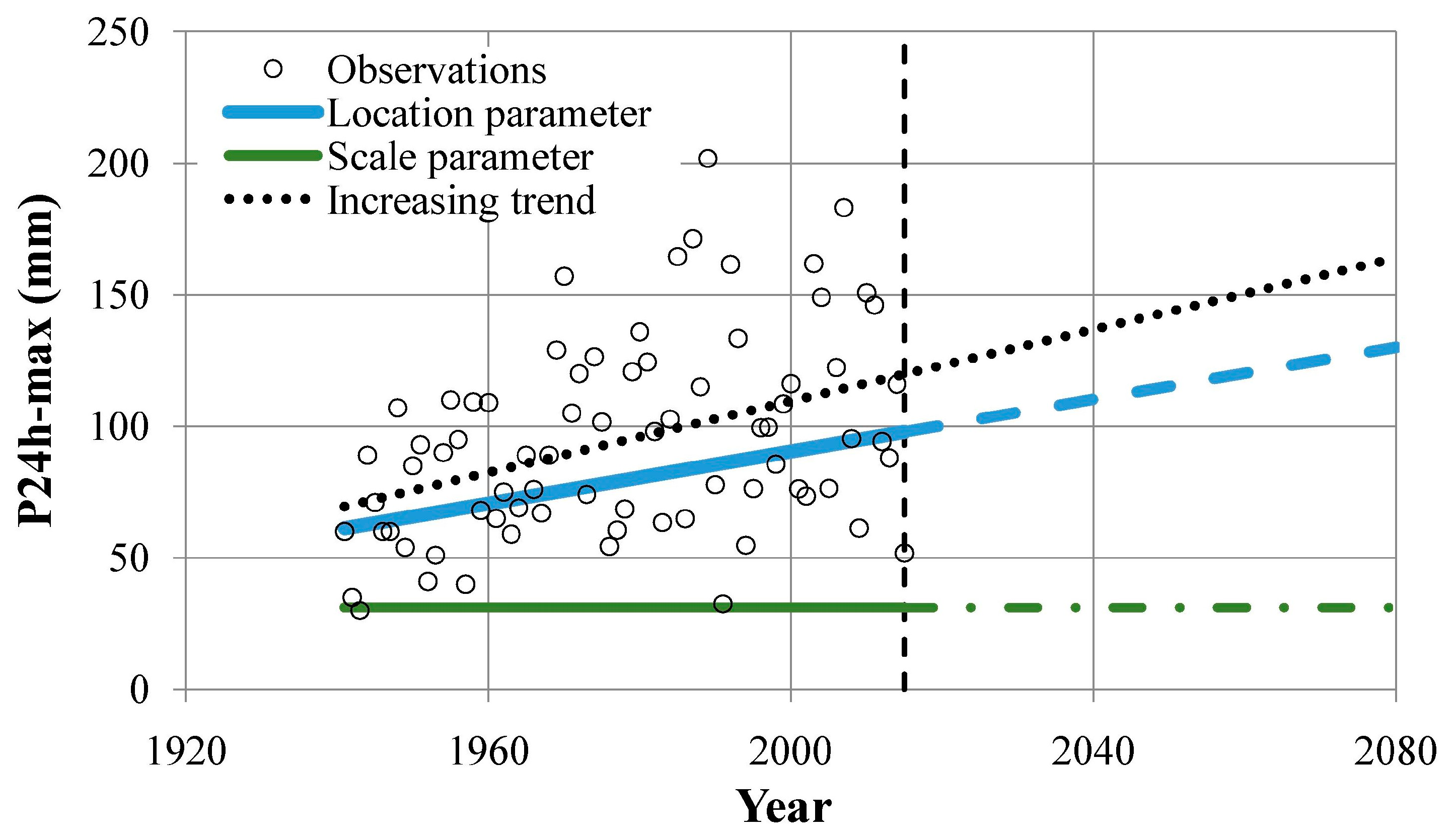
The analysis of the multiannual P_24h-max observations recorded at the Rafael Núñez airport weather station not only evidenced an increasing trend (Figure 5), but also, in Table 3, it could be noticed that, before 1985 rainfall events above 148.1 mm (estimated rainfall value for a 10-year return period under stationary conditions in Table 4) just occurred once (in 1970). After 1985, rainfall events of that magnitude (or higher) have occurred nine times (2011 rainfall was included as it is close enough). Colombian legislation recommends a 50-year return period for the design of open channels for watersheds of an area less than 1000 ha [5]. In Table 4 and Table 5, the rainfall for this return period, even for stationary conditions, was estimated to be nearly 200 mm. However, in Table 3, a rainfall of 201.8 mm has been already recorded in 1989. From this, it may be inferred that any hydraulic structure to be designed for such return period should be also evaluated for a higher value to test its hydraulic performance.

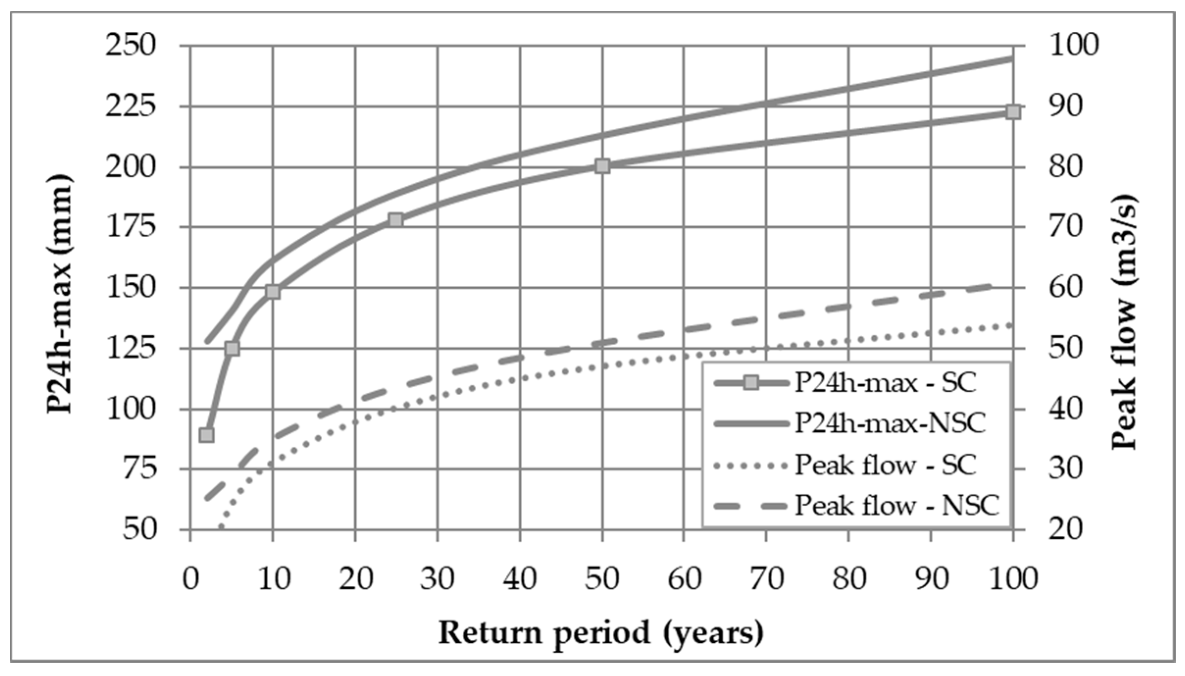
The estimated P_24h-max (Section 3.1 and Section 3.2) and the peak flow (Section 3.5) for several return periods under stationary and non-stationary conditions depicted in Figure 10 also showed an increase, from 6% to 44% for P_24h-max (

Table 10. P_24h-max values comparison.

Tr (year)	P24h-max (mm)			Ratio (NSC/SC)	Avg. Ratio
	SC	NSC	P24h-max Diff. (NSC-SC)
2	89.2	128.1	38.9	1.44
5	125.0	140.6	15.6	1.12	1.09
10	148.1	161.5	13.4	1.09
25	178.1	189.1	11.0	1.06
50	200.3	213.1	12.8	1.06
100	222.4	244.8	22.4	1.10

) and from 8% to 77% for peak flow (

Table 11. Peak flow values comparison.

Tr (year)	Peak Flow (m3/s)			Ratio (NSC/SC)	Avg. Ratio
	SC	NSC	Flow Diff. (NSC-SC)
2	14.3	25.3	11.0	1.77
5	24.3	29.0	4.7	1.19	1.12
10	31.2	35.2	4.0	1.13
25	40.2	43.6	3.4	1.08
50	47.1	51.0	3.9	1.08
100	53.9	60.9	7.0	1.13

), depending upon the return period. The increase seen in P_24h-max for return periods of 5 to 100 years are quite similar to each other, with an average value of 1.09. This value is in line with those observed in some areas of the Caribbean region of Colombia [6,7]. Despite the fact that a 44% increase in P_24h-max for the 2-year return period looks, at a glance, to be too high when compared to the remaining values, it may be construed as an indication that a more conservative approach might be conducted when designing with this low return period as the probability of exceeding is high.

For the peak flow, the values of the overall increase ratio have the same behavior of that shown by P_24h-max, with the maximum value occurring at a 2-year return period. A 44-percent increase in rainfall (Table 10) caused a 77-percent peak flow rise (Table 11). Once again, this indicates the precautions that the designers must take when using this return period. For the other return periods, it may be observed that the increase in P_24h-max resulted in a peak flow increase of a similar range.

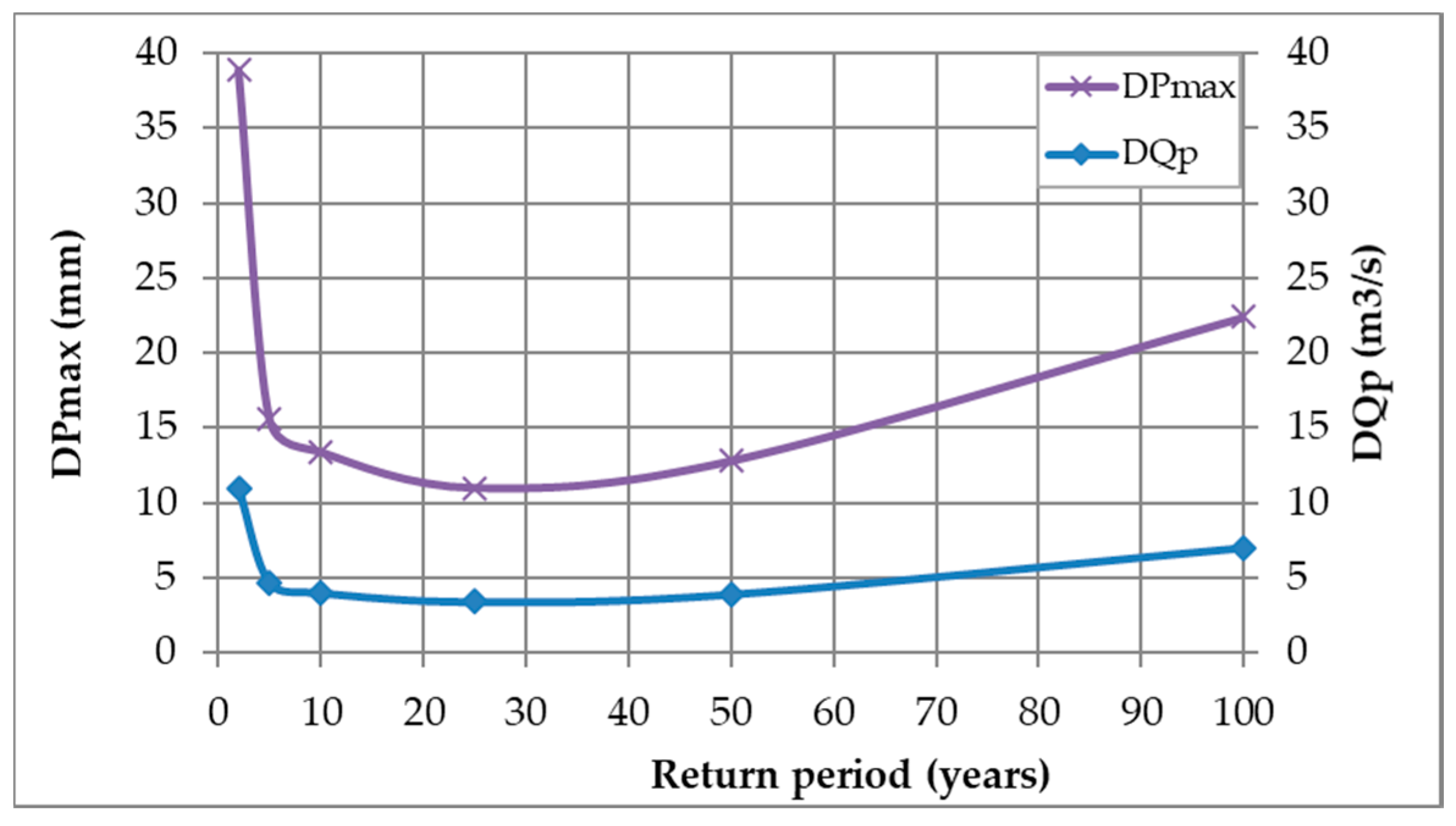
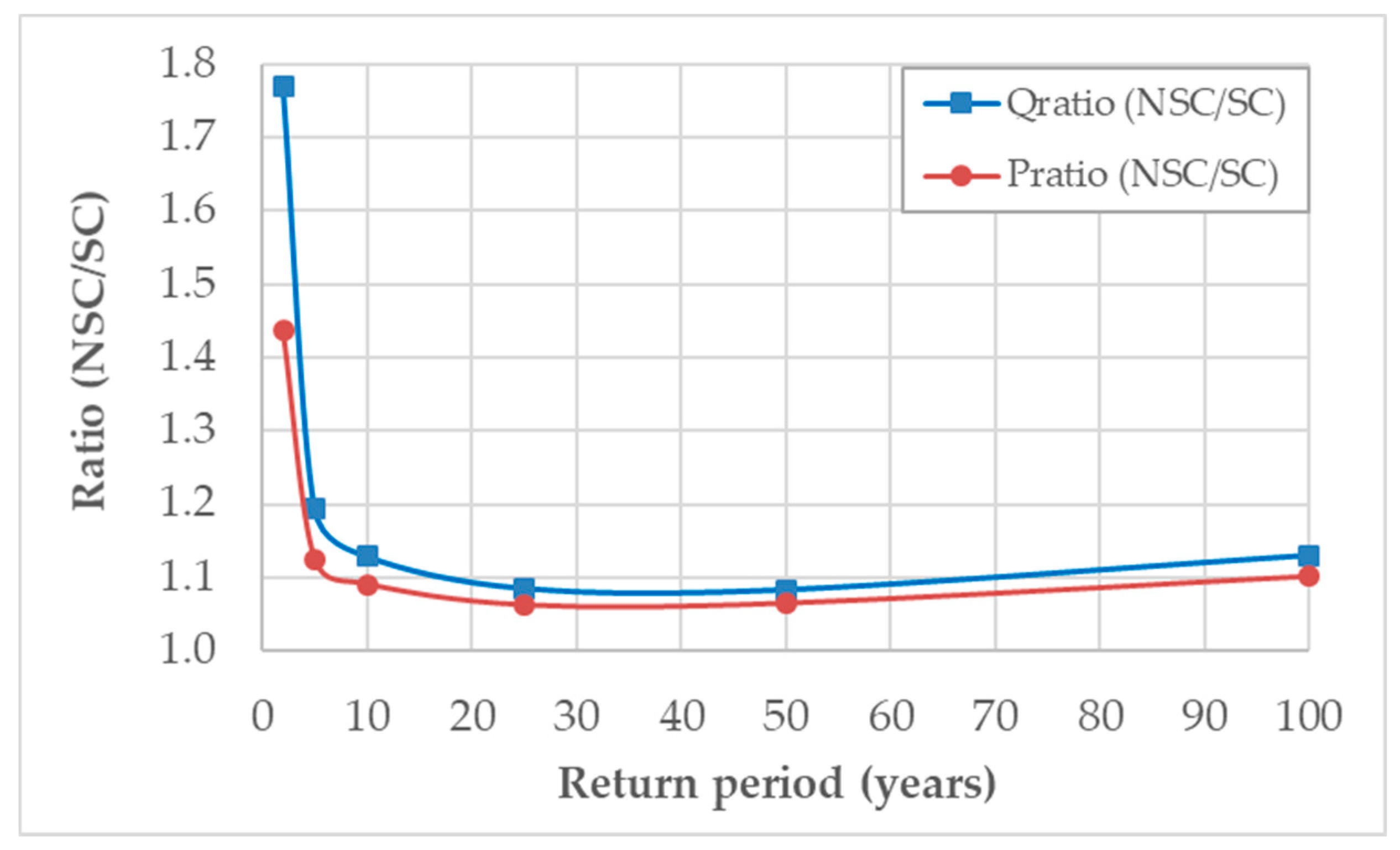
Figure 11 and Figure 12 show respectively the non-stationary and stationary difference and ratios between P_24h-max and peak flow for different return periods (DPmax, DQp, Pratio and Qratio). As expected, both show how the behavior of P_24h-max, and the watershed’s response to it (the peak flow), have the same trend.

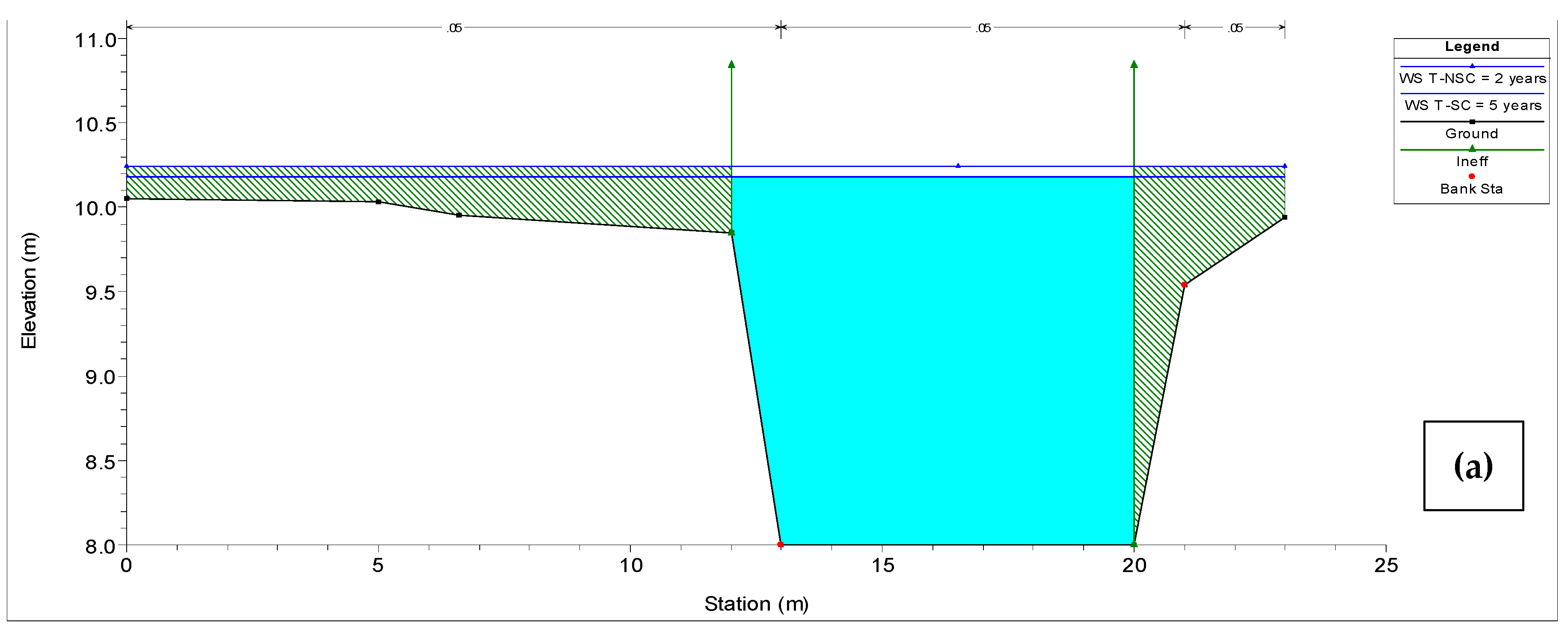
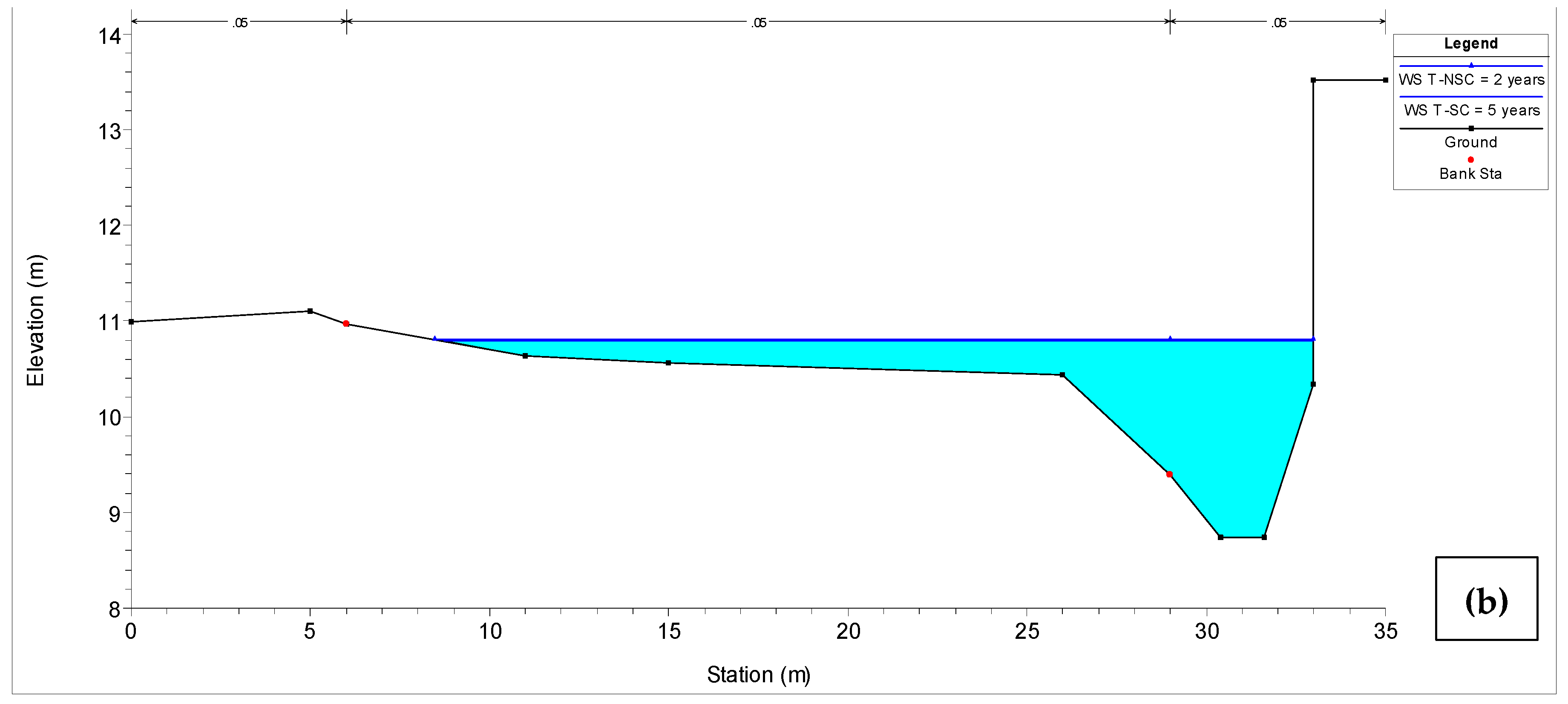
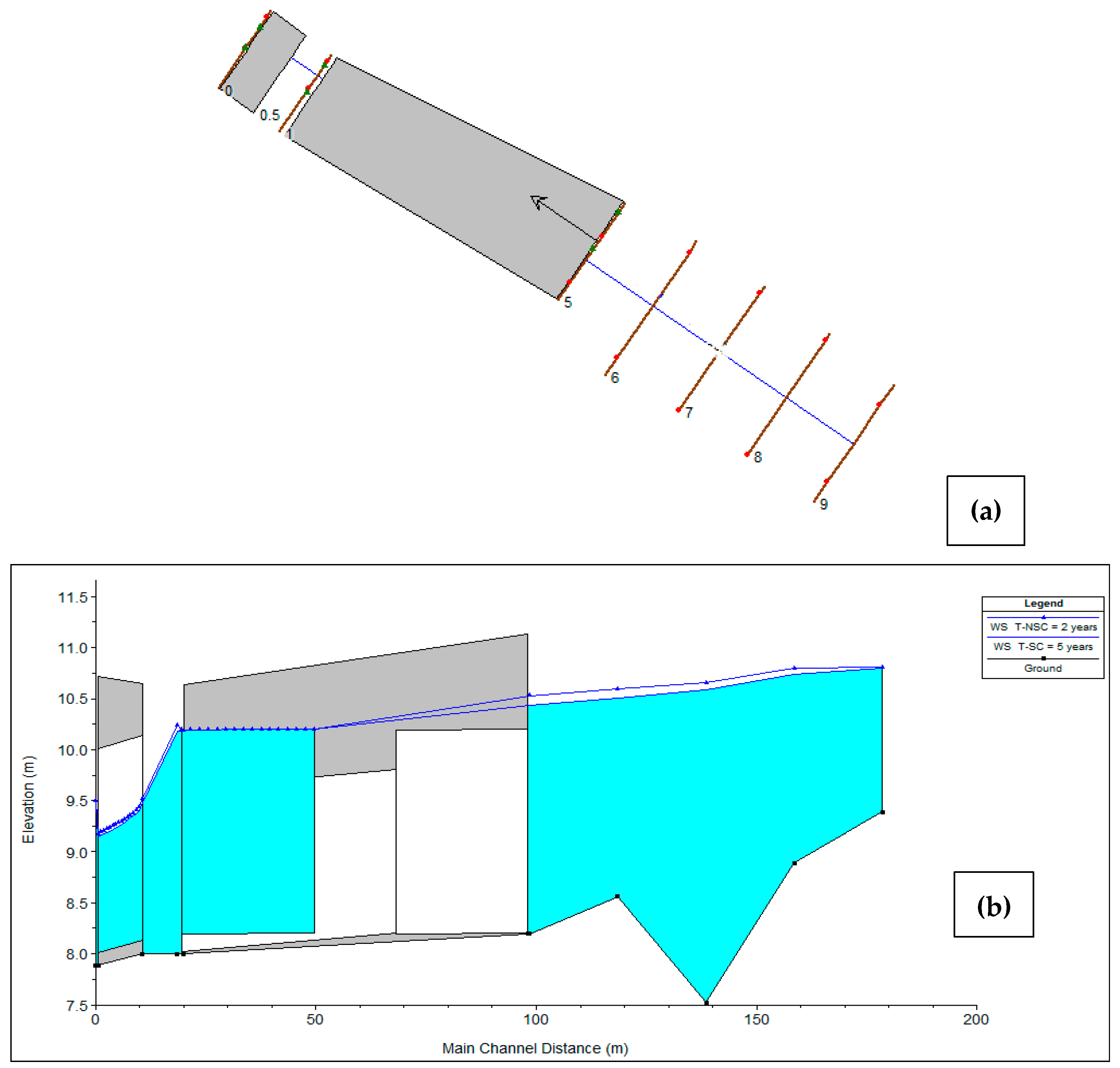
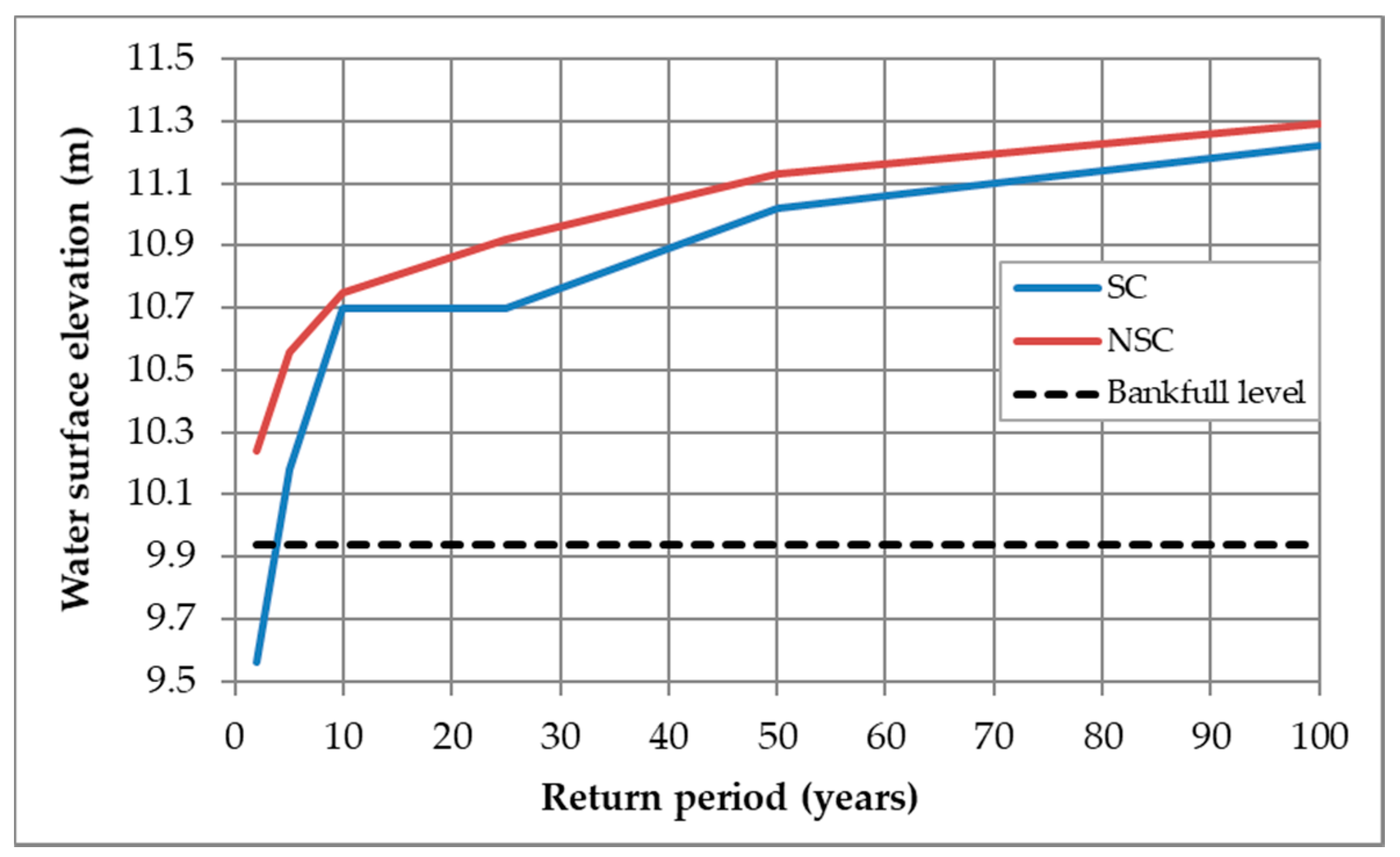
The water level reached after the simulations carried out under stationary and non-stationary conditions indicates that modeling under non-stationary scenario better represents the current hydrological conditions of the Gordo creek watershed, where rainfall events of low magnitude are generating floods every year during the rainy season (during which the soil is saturated most of the time) at the watershed’s outlet, when, in theory, they ought not to. This can be observed, for instance, in the results of the hydraulic simulation at K0+018.5 shown in

Table 12. Maximum water level (elevations) at cross-section K0+018.5.

Bankfull Elev. Is at 9.94 m		Max. Water Level Elevation Reached at Peak Flow
		Tr
		2	5	10	25	50	100
SC	P24h-max (mm)	89.2	125.0	148.1	178.1	200.3	222.4
	Q (m3/s)	14.3	24.3	31.2	40.2	47.1	53.9
	Water elev. (m)	9.56	10.18	10.70	10.70	11.02	11.22
NSC	P24h-max (mm)	128.1	140.6	161.5	189.1	213.1	244.8
	Q (m3/s)	25.3	29.0	35.2	43.6	51.0	60.9
	Water elev. (m)	10.24	10.56	10.75	10.92	11.13	11.29
Water elev. difference (m)		0.68	0.38	0.05	0.22	0.11	0.07

Values in bold indicate which year (return period) first exceeded the bankfull level under SC and NSC.

(P_24h-max, peak flow, and water elevation) and Figure 13, where the bankfull level (9.94 m) is reached at a lower return period (floods occur more frequently) under non-stationary conditions (Tr < 2-year). Under stationary conditions, a 2-year return period flow, defined as the mean annual flow (or annual maximum daily flow) [28,29], did not result in a bankfull section, which is not what is currently occurring in the study area (floods every year). The change in the rainfall pattern evidenced in previous sections may be the reason for a shift towards more recurrent and higher-than-usual events that cause floods more frequently than in the past. Likewise, statistically speaking, the ACI results obtained in Section 3.2 (747.5103 for non-stationary and 753.3721 for stationary) demonstrated that the non-stationary condition is more adequate. The AIC test serves to evaluate how good a model is for predicting future values [30]. The lower the value of the AIC the better the model.

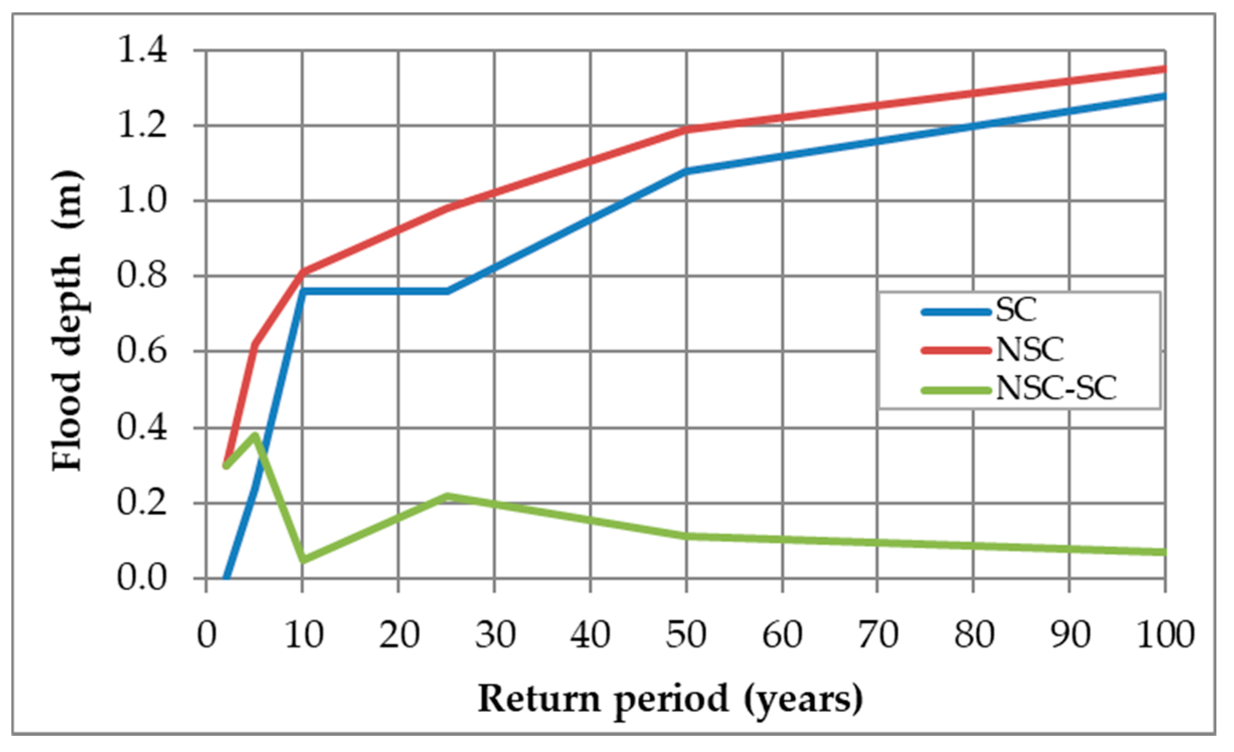
In terms of the flood depth (elevation above bankfull level) at the area of the watershed outlet,

Table 13. Flood depth at cross-section K0+018.5.

Flood Depth (m)
Tr (year)	SC	NSC	NSC-SC
2	0.00	0.30	0.30
5	0.24	0.62	0.38
10	0.76	0.81	0.05
25	0.76	0.98	0.22
50	1.08	1.19	0.11
100	1.28	1.35	0.07

Values in bold indicate which return period first exceeded the bankfull level under SC and NSC.

and Figure 14 show the water depth above the bankfull level for different return periods. This sensitivity analysis reveals the necessity for sizing hydraulic structures under non-stationary conditions to avoid more recurring floods. Notwithstanding that the 1-D hydraulic simulation is incapable of delineating the extension of the flooded area beyond the creek’s bank, the difference between NSC and SC elevations in Table 13 is an indication of what locals and workers of the industrial area have been noticing every year: floods in this area have been gradually worsening in terms of both frequency of occurrence and area covered by water (as well as the water depth marks left at some points that local people use as reference points). Further research is needed, though. Future work in this area must include a more detailed survey (topographic study) covering more area, so as to assess and more accurately quantify (numerically and spatially) the aforementioned anecdotal evidence.

An option for making decisions when designing some hydraulic structures would be to perform a benefit-cost analysis to compare a design under non-stationary conditions versus under stationary condition, taking into account free board heights, allowing handling of the non-stationary peak flow depending on the design return period.

In addition to the already quantified effects of climate change on Cartagena’s P_24h-max pattern and the Gordo creek watershed’s hydrological response, the fact that almost 85% of the watershed is still rural indicates that any increase in the impervious area will both raise the peak flow and reduce the time of concentration. These two variables will worsen the situation at the outlet of Gordo creek watershed unless a series of measures are implemented. For instance, the combination of sustainable urban drainage systems (SUDS) [31,32], stormwater storage vaults/tanks (both online and offline), aquifer storage and recovery (ASR) wells, infiltration ponds, among others, have proved to be effective at managing stormwater by: (a) keeping the peak flow at the same magnitude (or lower) when pre-development and post-development scenarios are compared, (b) avoiding the design of larger hydraulic structures, (c) minimizing the risk of floods, and (d) recharging aquifers, as a plus.

5. Conclusions

P_24h-max values associated to a given return period are a key variable when estimating design DSR for hydraulic structures for stormwater management, especially in ungauged watersheds. The values obtained in the AIC test carried out in this study, indicated that a frequency analysis under non-stationary conditions represents best the behavior of the rainfall patterns of the P_24h-max observations at the Rafael Núñez station. A stationary scenario is, in this case, further from the natural reality, when compared to non-stationary conditions. This was also confirmed by both the increase in the occurrence of P_24h-max events greater than or equal to 148.1 mm (value for a 10-year return period under stationary conditions), and the increasing linear trend over time of the overall P_24h-max observations. These findings may be an indication that the typical frequency analysis of rainfall under stationary conditions may no longer be applicable when calculating the design rainfall associated with a given return period for sizing hydraulic structures throughout Cartagena de Indias. Furthermore, designing under stationary conditions may have direct implications in the decisions local authorities will be taking in the coming years, given that millions of dollars will be invested in upgrading the city’s stormwater system. The 1-D hydraulic simulation performed herein revealed that the Gordo creek watershed outlet area can be flooded even with an event of 2-year return period (every year)—a situation that had never been observed in the past according to what local people have affirmed. The increase in the P_24h-max, though, is not the sole factor to be taken into account when evaluating the reasons behind the more frequent floods reported. Uncontrolled and unplanned urbanization of vegetated areas may and will exacerbate the recurrent floods registered within the study area.

It is noteworthy to mention that sizing larger hydraulic structures for stormwater management as the only solution for the larger rainfall events estimated under non-stationary conditions might be unsuitable and unsustainable in cases where surface area limitations exist (especially in urban areas). Therefore, implementing best management practices for controlling stormwater sources in old and newly constructed areas shall be one of the city’s goals in maintaining the design peak flow values, especially under increasing non-stationary conditions.

References

1. Faber, B. Current methods for hydrologic frequency analysis. In Proceedings of the Workshop on Nonstationarity, Hydrologic Frequency Analysis, and Water Management, Boulder, CO, USA, 13–15 January 2010; pp. 33–39. Available online: http://www.cwi.colostate.edu/nonstationarityworkshop/index.shtml (accessed on 21 December 2017).
2. Obeysekera, J.; Salas, J.D. Quantifying the uncertainty of design floods under nonstationary conditions. J. Hydrol. Eng. 2014, 19, 1438–1446. [Google Scholar] [CrossRef]
3. Wang, D.; Hagen, S.C.; Alizad, K. Climate change impact and uncertainty analysis of extreme rainfall events in the Apalachicola River basin, Florida. J. Hydrol. 2012, 480, 125–135. [Google Scholar] [CrossRef]
4. Salas, J.D.; Obeysekera, J.; Vogel, R.M. Techniques for assessing water infrastructure for nonstationary extreme events: A review. Hydrol. Sci. J. 2018. [Google Scholar] [CrossRef]
5. Ministry of Housing, City, and Development (MinVivienda); Republic of Colombia. Resolution 0330 of 8 June 2017, Technical Guidelines for the Sector of Potable Water and Basic Sanitation (RAS). 2017. Available online: http://www.minvivienda.gov.co/ResolucionesAgua/0330%20-%202017.pdf (accessed on 28 October 2017).
6. Poveda, G.; Alvarez, D.M. The collapse of the stationarity hypothesis due to climate change and climate variability: Implications for hydrologic engineering design. Rev. Ing. Univ. Andes 2012, 36, 65–76. [Google Scholar]
7. IDEAM, PNUD, MADS, DNP, CANCILLERÍA. New Scenarios of Climate Change for Colombia 2011–2100 Scientific Tools for Deparment-based Decision Making—National Emphasis: 3rd National Bulletin on Climate Change. 2015. Available online: http://documentacion.ideam.gov.co/openbiblio/bvirtual/022964/documento_nacional_departamental.pdf (accessed on 28 October 2017).
8. Chow, V.T.; Maidment, D.R.; Mays, L.W. Applied Hydrology, 1st ed.; McGraw-Hill: New York, NY, USA, 1988; pp. 350–376. [Google Scholar]
9. Palutikof, J.P.; Brabson, B.B.; Lister, D.H.; Adcock, S.T. A review of methods to calculate extreme wind speeds. Meteorol. Appl. 1999, 6, 119–132. [Google Scholar] [CrossRef]
10. Wilks, D.S. Statistical Methods in the Atmospheric Sciences, 3rd ed.; Academic Press: Oxford, UK; Waltham, MA, USA, 2011; pp. 105–110. [Google Scholar]
11. Gumbel, E.J. The return period of flood flows. Ann. Math. Stat. 1941, 2, 163–190. [Google Scholar] [CrossRef]
12. Frechet, M. Sur la loi de probabilité de l’ecart máximum (On the probability law of maximum values). Ann Soc. Pol. Math. 1927, 6, 93–116. [Google Scholar]
13. Weibull, W. A statistical theory of the strength of materials. In Proceedings of the Ingeniors Vetenskaps Akademien (The Royal Swedish Institute for Engineering Research) No. 51, Stockholm, Sweden; 1939; pp. 5–45. Available online: http://www.scirp.org/%28S%28czeh2tfqyw2orz553k1w0r45%29%29/reference/ReferencesPapers.aspx?ReferenceID=1923153 (accessed on 19 April 2018).
14. Pearson, K. On the systemic fitting of curves to observations and measurements. Biometrika 1902, 1, 265–303. [Google Scholar] [CrossRef]
15. Kolmogorov, A.N. Sulla determinazione empirica di una legge di distribuzione. G. Inst. Ital. Attuari 1933, 4, 83–91. [Google Scholar]
16. Smirnov, N.V. Estimate of deviation between empirical distribution functions in two independent samples. Bull. Moscow Univ. 1939, 2, 3–16. [Google Scholar]
17. Smirnov, N.V. Table for estimating the goodness of fit of empirical distributions. Ann. Math. Stat. 1948, 19, 279–281. [Google Scholar] [CrossRef]
18. Obeysekera, J.; Salas, J.D. Frequency of recurrent extremes under nonstationarity. J. Hydrol. Eng. ASCE 2016, 21. [Google Scholar] [CrossRef]
19. Akaike, H. A new look at the statistical model identification. IEEE Trans. Autom. Control 1974, 19, 716–723. [Google Scholar] [CrossRef]
20. USDA-Soil Conservation Service (USDA SCS). National Engineering Handbook, Section 4, Hydrology (NEH-4); USDA-SCS: Washington, DC, USA, 1985. Available online: https://policy.nrcs.usda.gov/OpenNonWebContent.aspx?content=18393.wba (accessed on 17 November 2017).
21. USDA Natural Resources Conservation Service (USDA NRSC). Conservation Engineering Division. Urban Hydrology for Small Watersheds, Technical Release 55 (TR-55); USDA-NRCS: Washington, DC, USA, 1986. Available online: https://www.nrcs.usda.gov/Internet/FSE_DOCUMENTS/stelprdb1044171.pdf (accessed on 19 December 2017).
22. Mishra, S.K.; Singh, V. Soil Conservation Service Curve Number (SCS-CN) Methodology, 1st ed.; Springer: Dordrecht, The Netherlands, 2003. [Google Scholar]
23. Ponce, V.M.; Hawkins, R.H. Runoff curve number: Has it reached maturity? J. Hydrol. Eng. ASCE 1996, 1, 11–19. [Google Scholar] [CrossRef]
24. Gericke, O.J.; Smithers, J.C. Review of methods used to estimate catchment response time for the purpose of peak discharge estimation. Hydrol. Sci. J. 2014, 59, 1935–1971. [Google Scholar] [CrossRef]
25. Sharifi, S.; Hosseini, S.M. Methodology for identifying the best equations for estimating the time of concentration of watersheds in a particular region. J. Irrig. Drain. Eng. ASCE 2011, 137. [Google Scholar] [CrossRef]
26. Kirpich, Z.P. Time of concentration of small agricultural watersheds. Civ. Eng. 1940, 10, 362–368. [Google Scholar]
27. Gonzalez, A.; Temimi, M.; Khanbilvardi, R. Adjustment to the curve number (NRCS-CN) to account for the vegetation effect on hydrological processes. Hydrol. Sci. J. 2015, 60, 591–605. [Google Scholar] [CrossRef]
28. U.S. Geological Survey (USGS). Flood-frequency Analyses, Manual of Hydrology: Part 3, Flood-flow Techniques; Government Printing Office: Washington, DC, USA, 1960. Available online: https://pubs.usgs.gov/wsp/1543a/report.pdf (accessed on 17 December 2017).
29. U.S. Geological Survey (USGS). Theoretical Implications of under Fit Streams, Flood-flow Techniques; Government Printing Office: Washington, DC, USA, 1965. Available online: https://pubs.usgs.gov/pp/0452c/report.pdf (accessed on 17 December 2017).
30. Mohammed, E.A.; Far, B.H. Emerging Business Intelligence Framework for a Clinical Laboratory Through Big Data Analytics 2015. Chapter 32. pp. 577–602. Available online: https://doi.org/10.1016/B978-0-12-802508-6.00032-6 (accessed on 28 January 2018).
31. Ramos, H.M.; Pérez-Sánchez, M.; Franco, A.B.; López-Jiménez, P.A. Urban Floods Adaptation and Sustainable Drainage Measures. Fluids 2017, 2, 61. [Google Scholar] [CrossRef]
32. New York City Department of Environmental Protection. Guidelines for the Design and Construction of Stormwater Management Systems; New York City Department of Environmental Protection: New York, NY, USA, 2012. Available online: http://www.nyc.gov/html/dep/pdf/green_infrastructure/stormwater_guidelines_2012_final.pdf (accessed on 4 January 2018).
Figure 1. Study area location.
Fluids 03 00027 g001
Figure 2. Study area location.
Fluids 03 00027 g002
Figure 3. (a) Access road to industrial area (2007); (b) Bus stranded in flooded area (2007); (c) Box-culvert (watershed outlet at cross-section K0+00) (2015); (d) Area downstream of the watershed outlet (2010). The locations where the pictures were taken are shown in Figure 2.
Fluids 03 00027 g003
Figure 4. Proposed methodology flowchart.
Fluids 03 00027 g004
Figure 5. P24h-max and GEV parameters (location and scale) behavior over time (Rafael Núñez airport station).
Fluids 03 00027 g005
Figure 6. 3-h rainfall distribution pattern at Rafael Núñez airport weather station.
Fluids 03 00027 g006
Figure 7. Plant view of the critical point of flooding.
Fluids 03 00027 g007
Figure 8. Natural cross-sections of Gordo creek. (a) Cross-section at K0+018.5; (b) cross-section at K0+178.5. WS indicates the water surface level.
Fluids 03 00027 g008aFluids 03 00027 g008b
Figure 9. Hydraulic modeling with HEC–RAS: (a) Plan view; (b) longitudinal profile. WS indicates the water surface level.
Fluids 03 00027 g009
Figure 10. P24h-max and peak flow increase for various return periods.
Fluids 03 00027 g010
Figure 11. P24h-max and peak flow variation for various return periods. DPmax and DQp are the P24h-max and peak flow difference between non-stationary and stationary conditions.
Fluids 03 00027 g011
Figure 12. P24h-max and peak flow ratio variation for various return periods. Qratio and Pratio are the ratio of non-stationary to stationary values of peak flow and P24h-max respectively.
Fluids 03 00027 g012
Figure 13. Water level at cross-section K0+018.5 for different return periods under stationary and non-stationary conditions.
Fluids 03 00027 g013
Figure 14. Flood depth at cross-section K0+018.5.
Fluids 03 00027 g014