Submesoscale Turbulence over a Topographic Slope

California Institute of Technology, 1200E California Blvd., Pasadena, CA 91125, USA
*
Author to whom correspondence should be addressed.
†
Current address: Israel Oceanographic and Limnological Research, Tel-Shikmona, Haifa 31080, Israel.
Fluids 2018, 3(2), 32; https://doi.org/10.3390/fluids3020032
Submission received: 27 December 2017
/
Revised: 29 April 2018
/
Accepted: 2 May 2018
/
Published: 7 May 2018
(This article belongs to the Collection Geophysical Fluid Dynamics)
Abstract
:Regions of the ocean near continental slopes are linked to significant vertical velocities caused by advection over a sloping bottom, frictional processes and diffusion. Oceanic motions at submesoscales are also characterized by enhanced vertical velocities, as compared to mesoscale motions, due to greater contributions from ageostrophic flows. These enhanced vertical velocities can make an important contribution to turbulent fluxes. Sloping topography may also induce large-scale potential vorticity gradients by modifying the slope of interior isopycnal surfaces. Potential vorticity gradients, in turn, may feed back on mesoscale stirring and the generation of submesoscale features. In this study, we explore the impact of sloping topography on the characteristics of submesoscale motions. We conduct high-resolution (1 km × 1 km) simulations of a wind-driven frontal current over an idealized continental shelf and slope. We explore changes in the magnitude, skewness and spectra of surface vorticity and vertical velocity across different configurations of the topographic slope and wind-forcing orientations. All of these properties are strongly modulated by the background topography. Furthermore, submesoscale characteristics exhibit spatial variability across the continental shelf and slope. We find that changes in the statistical properties of submesoscale motions are linked to mesoscale stirring responding to differences in the interior potential vorticity distributions, which are set by frictional processes at the ocean surface and over the sloping bottom. Improved parameterizations of submesoscale motions over topography may be needed to simulate the spatial variability of these features in coarser-resolution models, and are likely to be important to represent vertical nutrient fluxes in coastal waters.
1. Introduction
Dynamically, the transition between mesoscale and submesoscale motions is typically marked by the loss of geostrophic balance. This is in turn accompanied by the generation of larger vertical velocities through ageostrophic circulations, which occurs for [1]. Here, the Rossby number is the ratio of the vertical component of relative vorticity to the Coriolis frequency f. Previous studies have shown that submesoscale flows can influence vertical mixing [2], energy transport [3], biological productivity [4,5] and carbon export [6]. However, parameterizations of submesoscale dynamics are only now being implemented in global general circulation models (GCMs) [7], largely based on process studies in more idealized model configurations. Meanwhile, regional GCMs that directly resolve submesoscale motions show a potential increase in total eddy kinetic energy (EKE) by a factor of two [2,8] as compared to simulations where these motions are not resolved. The contribution of submesoscales to regional EKE may also exhibit seasonal cycles [9,10].
Motions at meso- and submesoscales are intricately linked as stirring by coherent mesoscale eddies are typically responsible either for frontogenesis or filamentation that produce lateral gradients that become susceptible to submesoscale instabilities [11,12]. Thus variations in the spatial and temporal scales of mesoscale motions may be reflected in the intensity of submesoscale flows. Variations in the depth of the mixed layer and the vertical stratification may also modulate submesoscale characteristics [13].
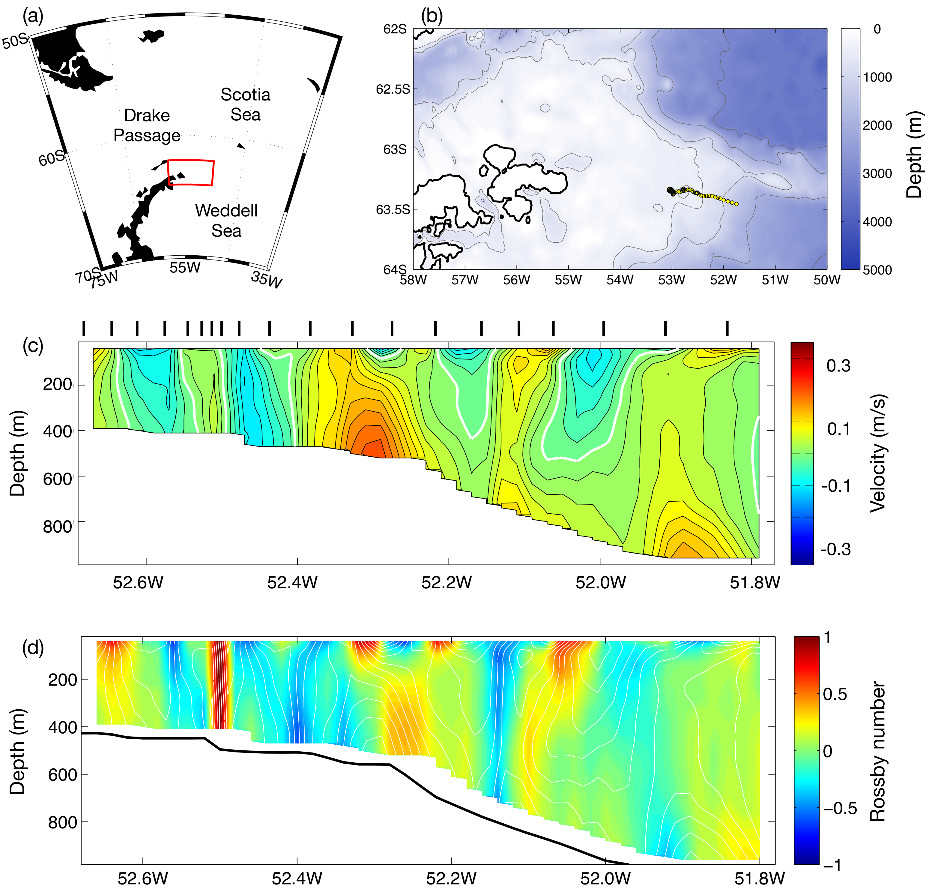
Large-scale topographic slopes focus frontal currents or jets, influence the extraction of potential energy via baroclinic instability and modulate the resulting equilibrated eddy kinetic energy (EKE) of ocean flows [14,15,16,17,18,19]. Topographic constraints on ocean variability are particularly strong at the continental margins with previous studies emphasizing the impact of topographic slopes on frontogenesis and jet stability [15,20,21]. Figure 1 shows an estimate of along a transect spanning the continental shelf and slope in the western Weddell Sea [22]. The vertical relative vorticity here is approximated by , where v and x are the cross-transect (along-slope) velocity and along-transect (cross-slope) distance respectively. This is a good approximation because in this region. The cross-transect velocity is calculated using the thermal wind relationship, referenced to the depth-averaged current from the glider, as documented in Thompson et al. [23]. The figure shows that often exceeds values of 0.5 and frequently reaches a magnitude of , suggesting that balanced geostrophic motion may be insufficient to describe dynamics here and in other parts of the ocean’s continental margins.
This observational data is also consistent with recent high-resolution numerical studies with a similar shelf-slope configuration. Stewart et al. [18,24] find that submesoscale eddies are generated over the continental shelf and shelf break, but are suppressed over the continental slope due to the strong potential vorticity gradient [17]. To date, much of the work on submesoscale dynamics has been limited to idealized processes models or observational studies in strong western boundary currents [25,26,27] and the open ocean [28]. Recently, however, studies on the influence of topographic slopes on submesoscale dynamics are beginning to emerge. A high resolution numerical model of the Gulf Stream, showed that energy is transferred from the geostrophic flow to submesoscale wakes through anticyclonic vertical vorticity generation in the bottom boundary layer. This provides a significant route to energy dissipation for geostrophic prograde boundary slope currents [29]. Using high-resolution hydrographic sections in southern Drake Passage, collected with autonomous ocean gliders, Ruan et al. [30] show that topographically-generated submesoscale flows over continental slopes enhance near-bottom mixing and that cross-density upwelling occurs preferentially over sloping topography. Here we look at idealized settings of similar along-slope currents, which will allow us to examine the submesoscale turbulence for different cases.
One common characteristic of submesoscale turbulence is the generation of ageostrophic motions that produce a significant asymmetry between cyclonic and anticyclonic coherent vortices. Both theoretical predictions [31,32] and laboratory experiments [33,34] have shown that anticyclonic vortices are more susceptible to inertial instability. This has been used to explain the preponderance of cyclonic submesoscale eddies observed at the ocean surface [35]. Furthermore, Eldevik and Dysthe [36] showed that ageostrophic baroclinic instability produces narrow frontal zones of strong cyclonic shear which roll up into submesoscale cyclonic eddies. Both of these mechanisms could explain the results of Capet et al. [12] and Klein et al. [3] who demonstrated in numerical simulations of the California Current system and a baroclinically-unstable zonal flow respectively, that submesoscale processes favor the generation of cyclonic vortices with larger than one. These results also hold in observations for open ocean regimes in which the fluid motion does not feel any additional constraints due to changes in the water column depth [37]. Here we explore the robustness of these asymmetries in topographically-controlled flows.
While this study largely focuses on the pattern of surface turbulence, it is known (and shown below) that surface characteristics are linked to potential vorticity (PV) distributions in the fluid interior. Modifications to PV are concentrated at the surface and sea floor due to surface wind forcing and bottom friction respectively. Thomas [38] showed that down-front wind forcing can extract PV from the fluid at the surface. The low PV is then transmitted through the boundary layer by the secondary circulation induced by the front [39]. Benthuysen and Thomas [40] proposed that bottom friction, responding to flow over a sloping bottom, could also inject or extract PV from the fluid depending on the direction of the mean flow. Bottom Ekman transport may induce changes in the isopycnal layer thickness and modulate PV in the fluid interior [23]. Finally, on larger scales, we also address the role of topography modifying the background PV, which changes the turbulence patterns.
In this manuscript, we explore the hypothesis that a sloping bottom topography has the potential to significantly modulate submesoscale characteristics of a turbulent ocean flow. We simulate an idealized wind-forced channel, which allows us to examine a range of surface wind-topography configurations. In Section 2, we present the model configuration and introduce five different experiments. In Section 3, we present results from the numerical simulations, focusing on vorticity distributions, vertical velocity and energy spectra, which are common methods of identifying submesoscale characteristics. We also discuss the relationship with larger-scale PV distributions. Discussions of these results and our conclusions follow in Section 4 and Section 5.
2. Model Description
The MIT global circulation model (MITgcm, Marshall and Radko [41], Marshall and Speer [42]) is employed to simulate a zonally-periodic channel on an f-plane, forced by a zonally-symmetric wind stress. A schematic figure, depicting the various model configurations, is shown in Figure 2. Since this study is partly motivated by data collected around the continental margins of Antarctica, the Coriolis parameter in the model is negative, defined as s−1. Typically, resolving submesoscale eddies requires the horizontal resolution on the order of one tenth of the Rossby deformation radius [5]. The model domain used in this study is 640 km in the meridional direction and 320 km in the zonal direction with a horizontal resolution of 1 km ×1 km. This scale is much smaller than the Rossby deformation radius, , where N is the buoyancy frequency ( s−1). These values produce a that varies between 10 km and 30 km, depending on the depth. In the vertical direction we have 60 layers evenly spaced from the surface to a maximum depth of m, giving a vertical resolution of 10 m. Density is a linear function of the potential temperature () with a constant thermal expansion coefficient (°C)−1. The initial θ (°C) profile is a function of latitude and depth,
where °C and km. We define to be the meridional mid-point of the channel. The surface temperature at the southern and northern boundaries of the domain are 15 °C and 23 °C, respectively. We provide a small perturbation to the initial temperature profile to induce baroclinic instability. At the northern and southern boundaries, relaxes to the initial stratification within a sponge layer of 20 km width. The relaxation time scale decays linearly to zero at the inner edge of the sponge layer with a maximum time scale of three days at the northern and southern boundaries. Sea surface is free and is initialized flat.
At the surface, we apply a meridionally-varying Gaussian wind stress
with the peak value N m−2 and a standard deviation of km. The momentum input by the wind stress is balanced by a linear bottom friction with a constant bottom drag coefficient, m s−1. In this model, horizontal and vertical viscosities are set to be 1 and m2 s−1 respectively. Horizontal and vertical temperature diffusion coefficients are 10 and m s−1, respectively. To simulate vertical mixing in the ocean surface boundary layer, the K-profile parametrization (KPP) method [43] is employed.
To study the influence of bathymetry, the simulations include a zonally-uniform topographic slope described by:
where m, m is the height of the slope relative to the maximum depth and km is the meridional scale of the slope. The ± sign indicates that the continental shelf, the shallowest part of which is 200 m, may be either in the north (−) or the south (+). Following Poulin and Flierl [15], we label the topographic slope as prograde when the shallow water is located to the left of the jet direction (recall that ); we label the topographic slope as retrograde when the shallow water is to the right of the jet direction. Unlike Poulin and Flierl [15], the jet direction is strongly forced by the surface wind stress, as opposed to responding to the propagation direction of topographic Rossby waves. The wind orientation is referenced to the initial temperature distribution. Down-front (DF) winds have the warmer water to the left of the wind stress maximum, while up-front (UF) winds have warmer water to the right of the wind stress maximum.
The parameter space we explore in this study is solely based on the relative orientation of the surface winds and the bathymetry. Experiments completed with different amplitudes of these properties showed qualitatively similar results. Based on alternating these two values, and including a “control” simulation with a flat bottom (DF-Fl), there are five different model configurations that are presented in Table 1 and Figure 2. In each experiment, the surface wind generates an along-slope current that is in the same direction as the wind stress. Thus, while configurations DF-S and DF-N both have a westerly wind stress and an eastward jet, they produce retrograde and prograde jets respectively because in the former, the shallow shelf region is to the south (S experiments) while in the latter the shelf is located to the north (N experiments). Similarly, configurations UF-S and UF-N produce prograde and retrograde jets respectively. Since the model simulates f-plane dynamics, the terms north and south have no strict dynamical meaning, however, the relaxation towards a colder boundary condition to the south sets the orientation of the large-scale background shear (consistent with south being poleward). In all of the simulations, this shear is positive .
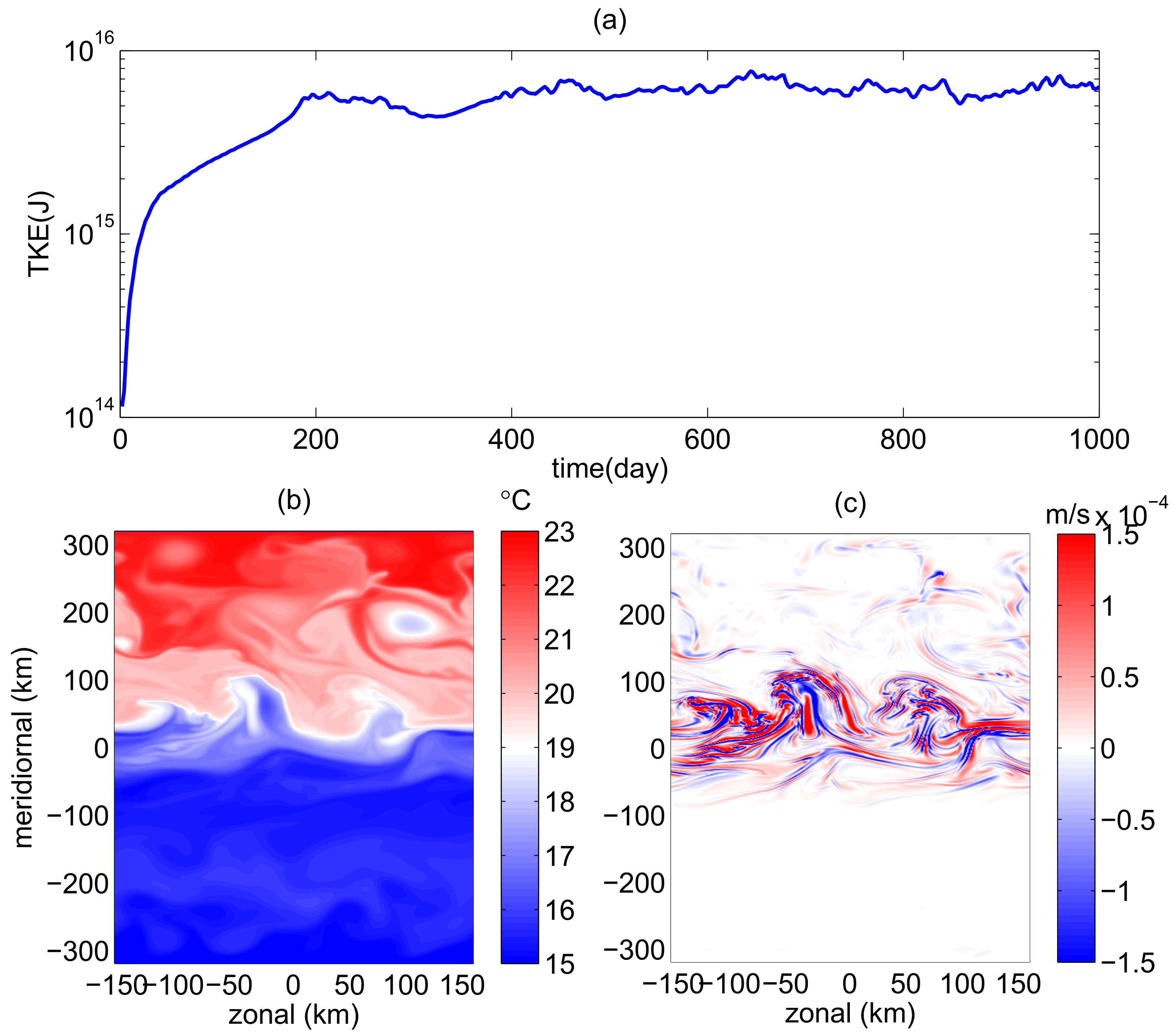
For each experiment described in Table 1, the simulation is integrated for a period of 1000 days. The initial velocity is zero everywhere in the domain. The time required to reach a statistically-equilibrated state depends on the model configurations, however, all model runs are equilibrated after 500 days. Equilibration is determined from considering the time series of total kinetic energy (TKE) (Figure 3a). Due to the suppression of linear instability growth rates over sloping topography [17], the experiments including a topographic slope take longer to reach equilibrium than the control experiment, DF-Fl. All calculations shown below represent averages over the last 200 days.
3. Results
Figure 3 provides an overview of Experiment DF-S. Available potential energy is present in all simulations due to the imposed initial temperature distribution. In experiments with down-front winds, Ekman pumping also contributes additional tilting of isopycnal surfaces. Baroclinic instability acts to relax this isopycnal tilt and generates mesoscale turbulence. Figure 3b shows a snaphot of surface at day 900; the sharp gradient just north of is indicative of frontogenesis with both mesoscale and submesoscale structures apparent. While mesoscale structure is largely associated with balanced, horizontal flow, Figure 3c provides strong evidence for an active and energetic submesoscale flow by showing a snapshot of the vertical velocity w at a depth of 30 m. Near-surface w has a large magnitude (up to 10 m/day) and displays fine filaments associated with ageostrophic fronts. A spatial pattern in the strength of w occurs (Figure 3c) with large absolute values of w over the deeper (northern) flank of the domain, while turbulence is suppressed over the shallow (southern) flank of the domain.
We focus on the non-linear statistically-equilibrated state, and do not analyze the spin-up or stability of the jets. The equilibrated structure of the jet depends on both winds and topography. Sloping topography creates large along-isopycnal PV gradients at the start of the experiment due to isopycnals incropping on the slope, resulting in vanishing layer thickness (see Figure 2). Wind forcing creates a mean overturning circulation. The homogenization of PV together with wind forcing determines the equilibrated stratification and jet structure. Stability analyses have been carried out for barotropic jets (e.g., Poulin and Flierl [15]), and for some simple cases for baroclinic jets [17,44]. However, these studies do not cover all aspects of our numerical simulations, for instance, the impact of a surface wind stress and the fact that density surfaces may incrop on the bottom topography. Isachsen [17] shows that a quasi-geostrophic (QG) stability analysis does not predict diffusivities diagnosed from primitive equation simulations well, while Poulin et al. [44] focus on prograde jets. In any case, in this paper we investigate the non-linear saturation, which is very different in these cases, especially with steep slopes [17,45].
The enhancement of vertical velocities is consistent with a transition towards flow with Rossby number. Figure 4 shows both time-averaged and snapshots of the surface (10 m) for each of the five experiments in Table 1. As in previous studies, we define local as the ratio of absolute vertical vorticity and planetary vorticity:
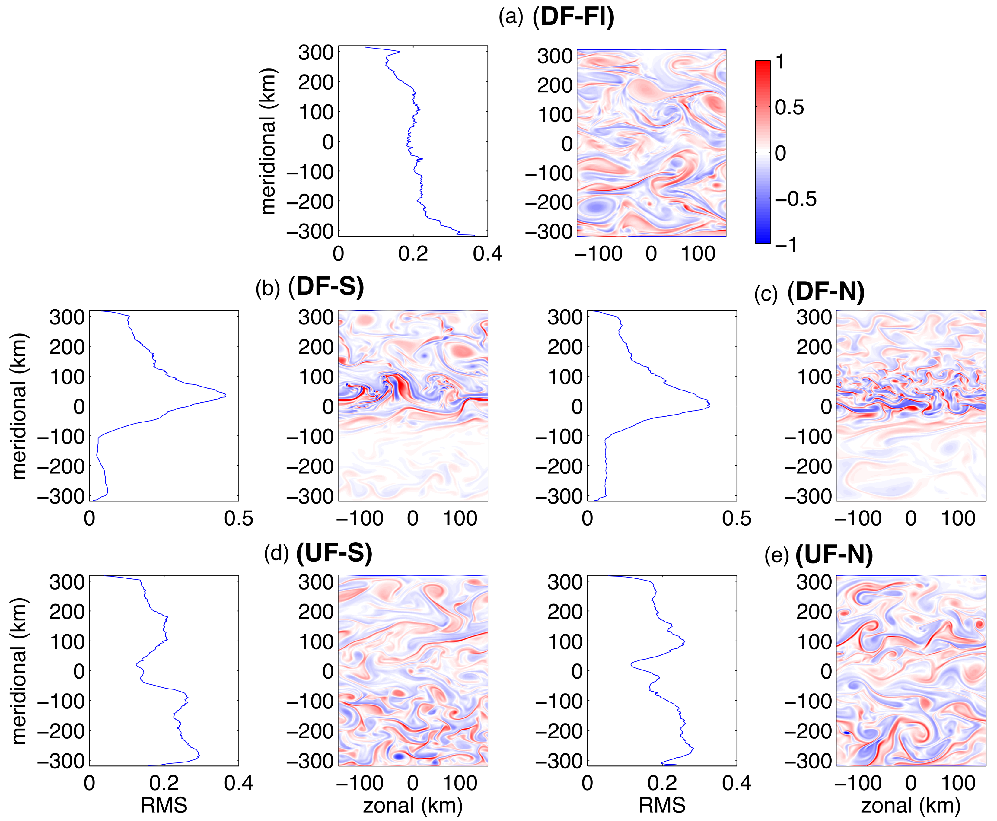
where is the velocity and is the vertical unit vector. In the snapshots the surface is frequently . Comparing the different experiments, we find the following features: (1) In all experiments, the domain is dominated by regions where is positive. (2) Simulations that have a topographic slope tend to exhibit structure on smaller scales compared to the DF-Fl Experiment (Figure 4a). (3) Furthermore, in all experiments with topography, the meso/submesoscale turbulence acquires an asymmetric meridional (warm-to-cold or deep-to-shallow) spatial pattern. For example, in Figure 4b,c, the down-front wind experiments, the warmer, “northern” flank is more energetic and exhibits larger values of . This is true even though the topographic orientation is reversed between these two experiments. In contrast, in Figure 4d,e, for the up-front wind experiments, the colder, “southern” flank of the jet is more energetic and exhibits larger values of . However, the meridional asymmetry is less dramatic in these up-front wind experiments. Since all other parameters are the same for these five experiments, Figure 4 indicates that the orientations of the surface wind stress and the bathymetric slope not only influence the amplitude of the submesoscale turbulence, but also its spatial patterns. (4) The time-averaged peaks in the core of the slope front current in both of the down-front wind experiments (Figure 4b,c), while it is suppressed in the core of the jet in the up-front wind experiments (Figure 4d,e). In contrast, is uniform with latitude, outside of the sponge layers, in the flat bottom Experiment (Figure 4a).
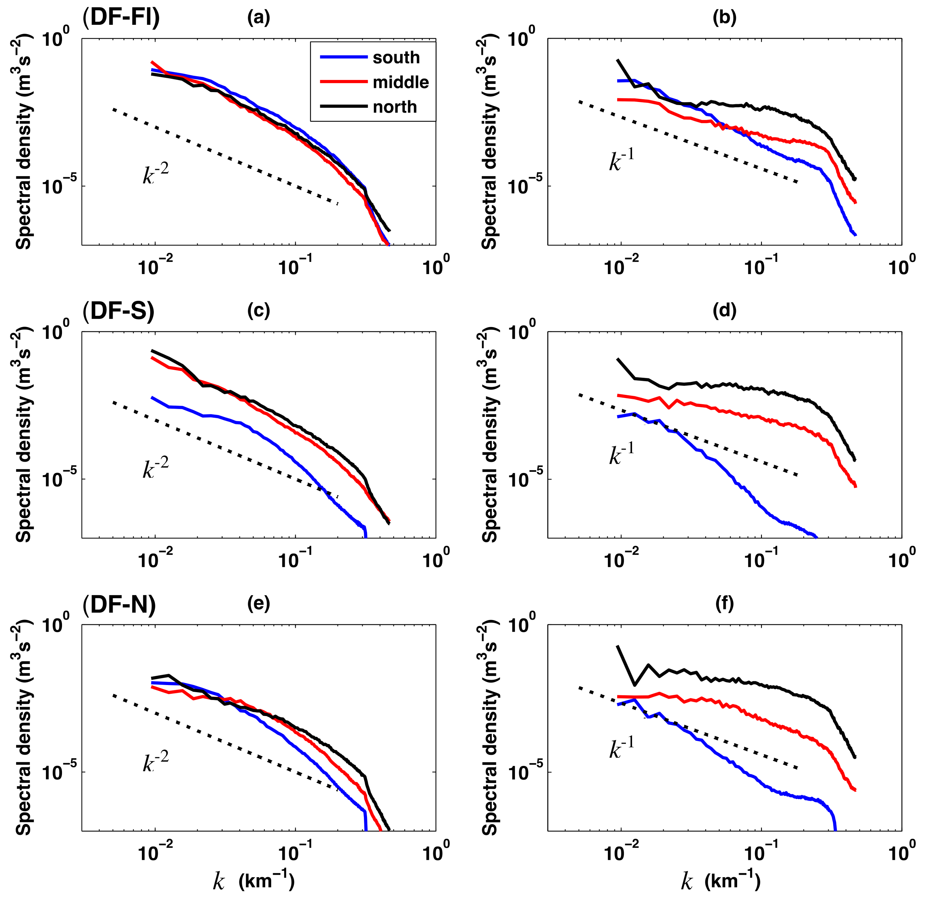
The meridional distribution of the turbulence can be further explored by considering the energy content at different spatial scales as shown by the power spectra of surface kinetic energy (KE) and vertical velocity (Figure 5). In each panel, the domain is partitioned into regions on the northern (black, ) and southern (blue, ) flanks of the jet as well as the jet cores (red, ). Overall, the surface KE spectra have slopes close to , while the vertical velocity spectra have slopes close to . The spectral slope is steeper in the interior deeper ocean (not shown, see Klein et al. [3]). For Experiment DF-S, the northern (warm) flank has a larger KE spectral amplitude. The northern flank also exhibits larger amplitude in the vertical velocity spectral curve, consistent with the asymmetry in Figure 4b. In addition to having a larger amplitude, Figure 5d also shows that the northern flank surface vertical velocity spectra has a slope of , which is significantly shallower than in all other simulations. A shallow slope implies that a greater proportion of energy is found at higher wavenumbers or smaller scales. In the control experiment, DF-Fl, surface KE and vertical velocity spectra do not show significant north to south differences in either amplitude or spectral slopes. The north-to-south asymmetry near the surface is largest in Experiment DF-S. The spectral slope in Experiment DF-N is similar to Experiment DF-S, although the amplitude is larger in DF-S. In the UF experiments, where the wind forcing is to the opposite direction of the thermal-wind balanced flow (Experiments UF-S, UF-N), the surface turbulence spectra is not modified as strongly by the bathymetry. Kinetic energy and vertical velocity spectra in Experiments UF-S and UF-N are similar to the control Experiment DF-Fl (not shown).
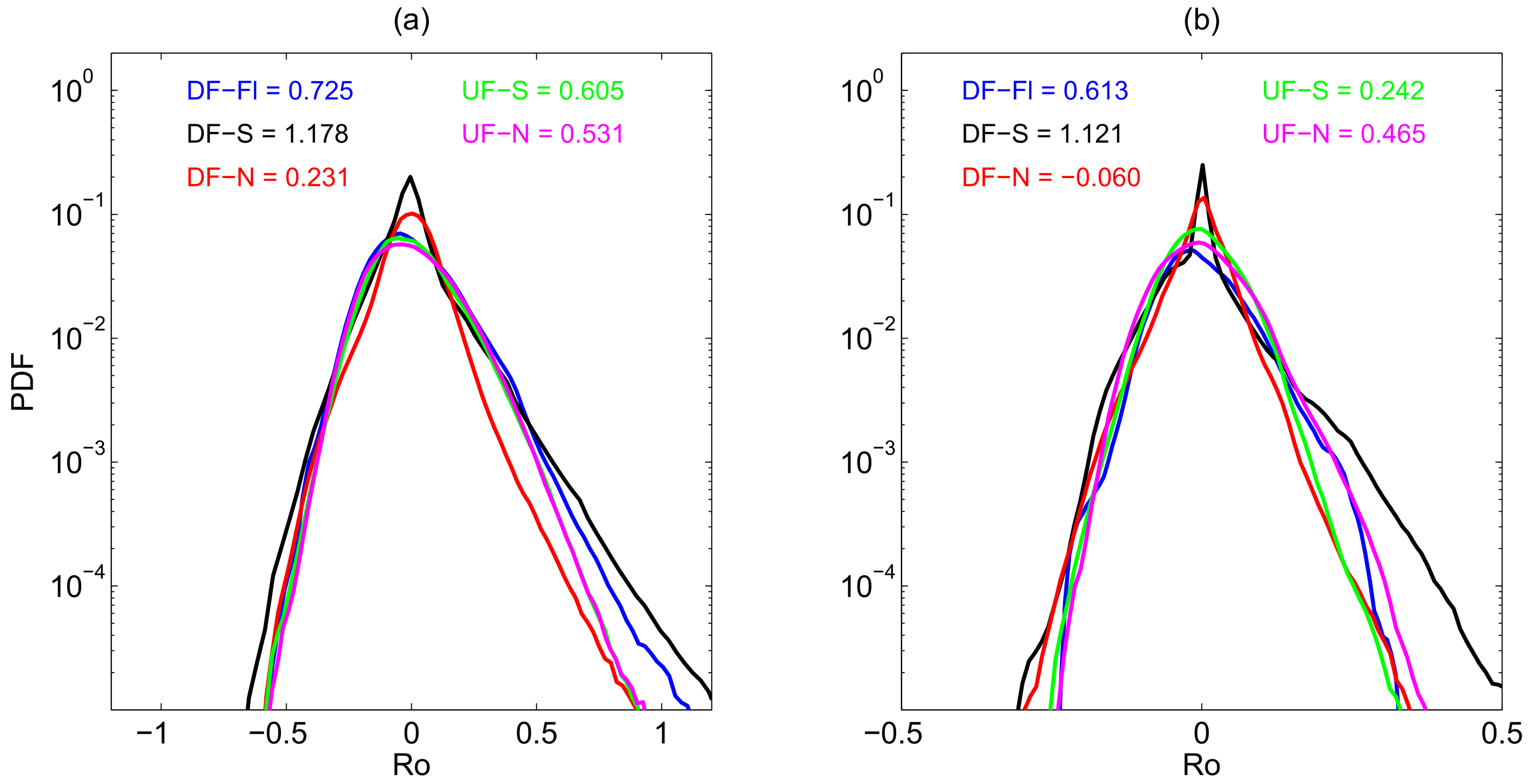
In all experiments, cyclonic vortices are more prevalent near the surface than anticyclonic vortices, resulting in a preference for positive . As mentioned in the introduction, this is consistent with many previous studies (Munk et al. [35], Lazar et al. [32], Buckingham et al. [37] to name a few), and is a possible signature of the flow’s geostrophic imbalance. In each of our simulations, we choose a shallow layer at 10 m depth and calculate the probability density functions (PDF) as shown in Figure 6a. The mean PDFs for all experiments show an asymmetric distribution between positive and negative values with larger tails on the positive side. The skewness, as measured by the third moment of , is positive in all experiments.
Away from the surface, decays to smaller values, roughly by a factor of 3 at 180 m depth (Figure 6b, also shown in Klein et al. [3]). PDF skewness of in the interior also decreases to smaller values compared to that close to the surface, and in DF-N, the skewness of decays altogether. The relative strength of the skewness across the different experiments remains unchanged away from the surface. The down-front wind experiments, DF-N and DF-S, exhibit the minimum and maximum values of the skewness parameter, respectively, both at the surface and in the interior. The mean of these values is approximately equal to the skewness that occurs in the flat bottom experiment. This is partially a feature of the influence of the topography on the skewness giving rise to regions within a single experiment where skewness is stronger or weaker.
The spatially-asymmetric pattern of the flow’s turbulent characteristics across the northern and southern flanks of the jet can be linked to the potential vorticity (PV) gradients in the fluid interior. The Ertel PV is defined as:
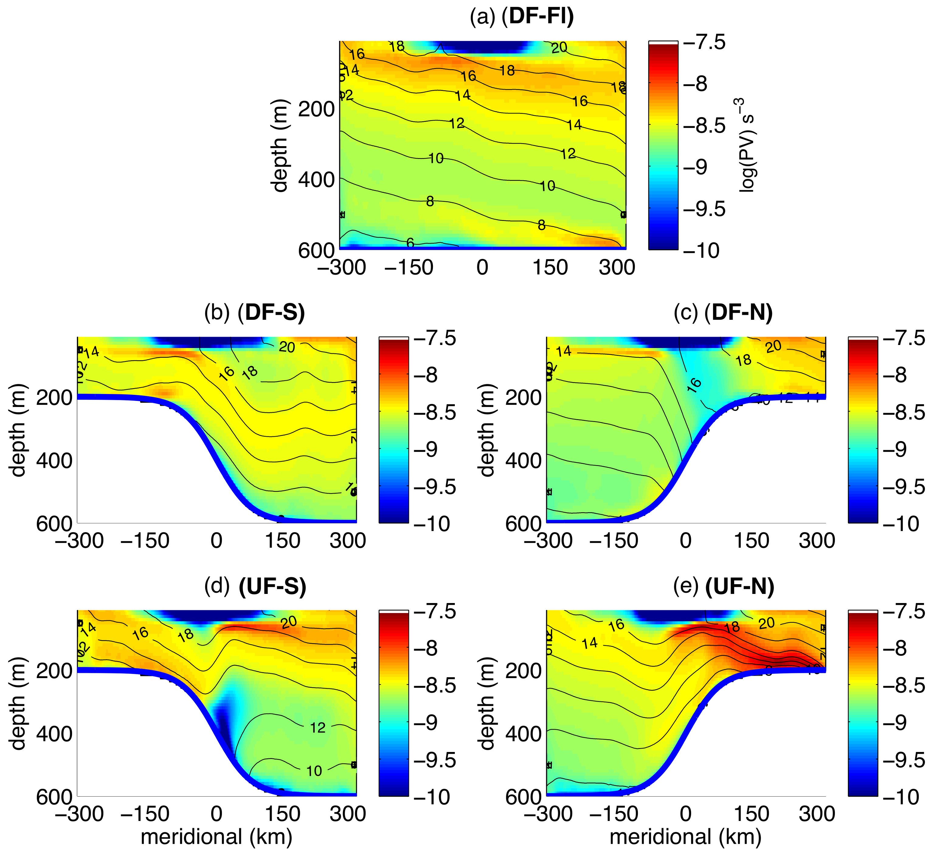
where the buoyancy b, is a linear function of in our model. The interior of the model domain is largely adiabatic, therefore we expect PV anomalies to be generated primarily at interfaces, for example due to the surface wind stress or bottom friction, or within the sponge layers at northern and southern boundaries. Figure 7 shows vertical cross sections of PV along with potential temperature contours for each experiment. Figure 8 shows PV projected onto different isopycnal (or isothermal) layers, in Experiment DF-S. Due to its large variations with depth, the absolute value of PV is shown with a logarithmic scale in Figure 7. Low PV is generated near the surface frontal regions due to wind stress, inducing lateral Ekman transport as well as strong vertical mixing. At the bottom, momentum input by the wind forcing is balanced by friction. At the same time, bottom friction drives Ekman transport to the right hand side of the zonal flow’s orientation. Therefore, in Experiments DF-S and UF-N, bottom Ekman transport increases stratification, moving dense water below light water, acting as a PV source (measured by the absolute value). In Experiments DF-N and UF-S, bottom Ekman transport decreases the stratification and extracts PV from the fluid, acting as a PV sink. The bottom PV sink is obvious on the slope in Experiment UF-S (Figure 7d). However, for the other experiments it is harder to detect the sources and sinks as PV values span three orders of magnitude. However, the PV source (in absolute value) at the incropping of the isopycnals with the slope in Experiment DF-S is apparent when looking at Figure 8a, which shows PV projected onto the 12 °C isopycnal. A strong (negative) PV source, is evident at the incropping point (at approximately −150 km South). Sources and sinks can be detected in experiments UF-N and DF-N respectively in the same way (not shown). These anomalies only occur on the isopycnal layers that directly intersect with the topography.
In the flat bottom Experiment DF-Fl, the PV structure is more uniform in the vertical direction. Critically, only a small temperature or density range outcrops on the bottom. The isopycnals that outcrop vary over relatively large scales (approximately the domain size). Thus, Ekman transport is unable to generate large PV anomalies near the bottom in this experiment. By comparing Experiment DF-Fl with other experiments, we also confirm that PV changes are mainly attributed to the modulation of bottom topographic slope, and not to the surface wind forcing alone.
In the interior, westerly wind in Experiments DF-S and DF-N creates an Ekman overturning circulation in the central area of the domain that tilts the isopycnal layers upslope in DF-S and downslope in DF-N. As a consequence, interior PV gradients are generated due to the change of isopycnal layer thickness. There is a correlation between the formation of submesoscale eddies and PV, in which these are formed preferentially on the flank of the jet where stratification is weak (low absolute value PV), and suppressed over the flank of the jet where the stratification is intensified (high absolute value PV). This can be seen in experiment DF-S in Figure 7b, where PV at −150 km South is higher ( varies between to ) than PV at 150 km North ( to ), which corresponds to a preference of submesoscale eddies in the northern flank of the jet. Figure 4b and Figure 5b both show that the turbulence is stronger and more energetic at smaller scales in the north than the south side of the jet. Similarly, in experiment DF-N there is higher PV on the southern flank () of the jet compared to the northern () in the central area of the domain. Correspondingly, Figure 4c shows more energetic and smaller scale turbulence in the northern flank of the jet as compared to the suppressed turbulence in the south. The spectra in Figure 5c averages the whole northern area of the domain, some of which has a high PV (north of 150 km), and therefore does not reflect this well. For the experiments where the winds are easterly (UF-S and UF-N), the PV gradient is in the other direction, with higher PV in the northern flank of the jet than the southern (Figure 7). Respectively, turbulence is more energetic and smaller in scale in the southern flank than in the north (as seen in Figure 4d,e, and more pronounced when looking at the left panels of the zonally and temporally averaged root mean squared Rossby number).
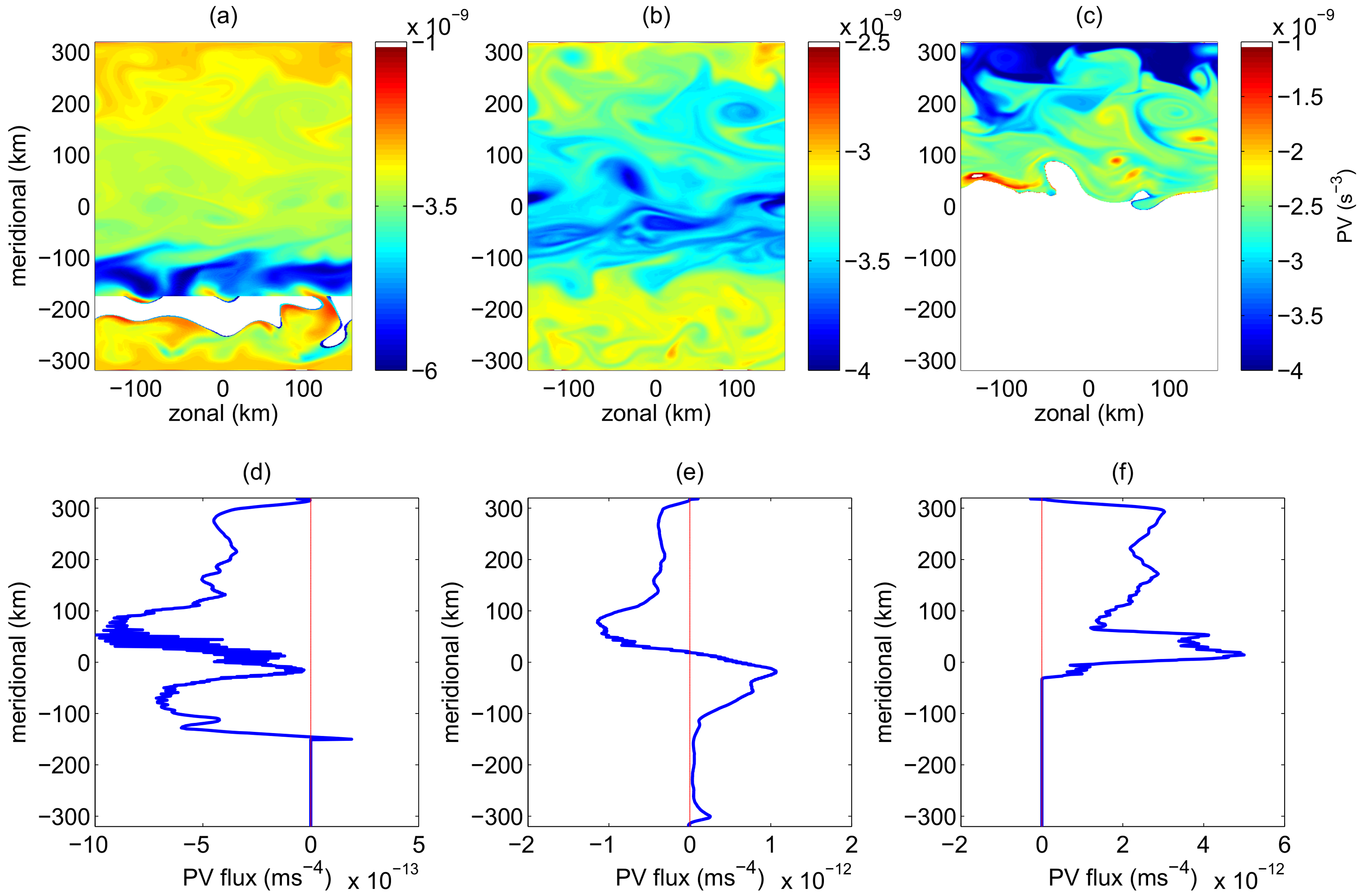
Figure 8 shows in the upper panels snapshots of coherent PV patterns from the bottom to the surface in Experiment DF-S. The instantaneous PV anomalies on the three layers shows similar patterns, related to either wind forcing at the surface or due to bottom friction. Corresponding time and zonal mean PV fluxes are also calculated in each isopycnal layer as , where is meridional velocity interpolated to the surface in each snapshot. The time-mean PV flux has the opposite sign to the PV gradient, as expected. Panel (a) shows that in the layer that intersects the slope, a negative PV anomaly is generated near the slope, which results in a negative PV flux that acts to homogenize PV on this layer. Panel (c) shows the pattern of the low absolute value PV seen in the surface of Figure 7b. On this surface, the PV flux is positive as the meridional PV gradient has reversed sign with depth. On the 14 °C isopycnal layer, which neither intersects with the surface nor the bottom on average, we see similar instantaneous PV patterns to the layers above and below (compare Figure 8b to Figure 8a,c). These are a result of the layer thickness modulations from above and below, which shows that PV sources/sinks at the bottom (top) due to Ekman transport can affect the stratification in the isopycnal layers above (below). Gradients on this layer may be sustained against the action of mesoscale stirring due to the sponge layers at the boundaries, where the vertical stratification is fixed and thus provide sources or sinks of PV. Furthermore, the density surface may intermittently outcrop (or incrop) at the flanks of the jet, thus, even if the time-averaged depth of the isopycnal does not outcrop at the surface or bottom, there could be a time-averaged source of PV that can give rise to the observed PV pattern. In the interior of an adiabatic fluid, away from sources and sinks, the flux should be constant; we expect deviations away from this constant flux may be due to insufficient averaging.
4. Discussion
4.1. Spectral Slope
The spectral representation of the velocity field has been a powerful tool for distinguishing flows in mesoscale and submesoscale regimes. At the outset of the study, we described the submesoscale range as those scales at which becomes and therefore, ageostrophic motions, by definition, become relevant. Callies and Ferrari [46], using an objective rather than a dynamic definition, identified submesoscales using a wavelength range from 1 to 200 km, and used observation-based spectra of eddy kinetic energy to determine the contribution from balanced and unbalanced motions at these scales. In the Gulf Stream region, within the mixed layer, a transition between balanced, interior quasi-geostrophic motion and unbalanced, predominantly internal wave motion, occurs at roughly 20 km. At scales smaller than 20 km, unbalanced motion was found to dominate the energy spectrum, and spectral slopes consistent with surface quasi-geostrophic (SQG) predictions [3] were not found. Additionally, in a more quiescent region in the eastern Pacific, kinetic energy distributions were not consistent with SQG, nor did they reveal a geostrophic turbulence regime (spectral slope of ). Callies and Ferrari [46] argued that the disagreement with SQG theory arose from the injection of energy in the submesoscale range by small-scale baroclinic instabilities or from a coupling between surface and interior dynamics.
Klein et al. [3] concluded that in near surface kinetic energy spectra show a slope, which is significantly shallower than that in the deeper ocean (). In our simulations, surface kinetic energy spectra show a similar slope of despite the introduction of a continental slope and wind forcing, which inject PV into the interior, breaking the conditions for SQG. However, for our simulations, we introduce a stratification that decays exponentially with depth, which should result in a kinetic energy slope that is flatter than (see Equation (A6) and Figure 3 of Callies and Ferrari [46]). Furthermore, the spectra show a weak dependence with depth, which also contradicts SQG theory. Thus we conclude that our shallow spectra are not results of near-surface SQG dynamics, but rather the result of the generation of unbalanced, ageostrophic motions.
Mixed layer baroclinic and symmetric instabilities may enhance submesoscale turbulence and flatten the spectra [12]. Additionally, while we do not resolve internal waves in these experiments, we speculate that the introduction of a topographic slope may impact the wavelength at which the transition between balanced and unbalanced motions occur. Both of these processes are likely to be active in producing the spectra diagnosed from our simulations.
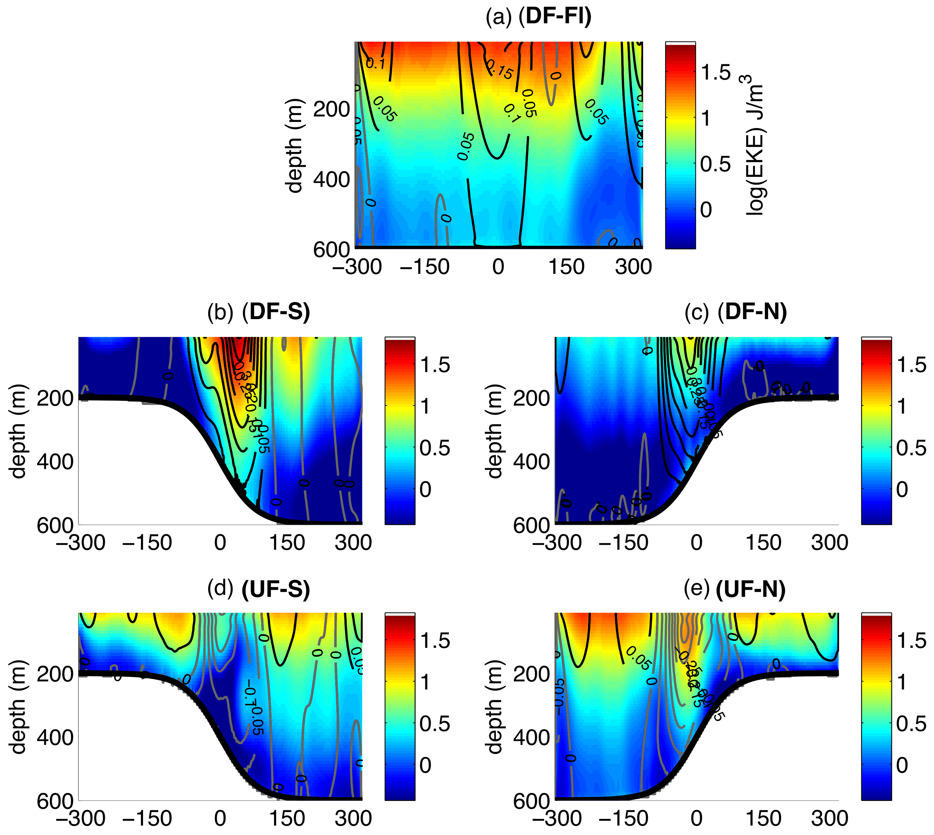
Typical explanations for the failure of geostrophic balanced motion include frontal circulations, Ekman flows, mixed layer turbulence, near-inertial oscillations, and internal tides. We can eliminate internal tides because they are not included in our simulations. However, both frontal circulations and Ekman flows are likely to play a critical part in generating the flatter spectra and also in explaining the diversity of spectral slopes seen across the different simulations. To assess the importance of Ekman flows and mixed layer turbulence, we have analyzed the vertical structure of the EKE in our various simulations (Figure 9). Experiment DF-N shows the largest degree of vertical decay of the EKE amplitude, where all the other experiments show similar levels of EKE throughout the upper 200 m of the domain. The DF-N experiment also shows the smallest vorticity skewness (Figure 6), which decays completely in only 180 m depth. This is also consistent with the fact that in Experiment DF-N, the PV is approximately constant throughout the water column (Figure 7).
Rosso et al. [47] studied the spatial inhomogeneity in submesoscale turbulence and proposed that topography influences submesoscale dynamics indirectly through the interaction with the large scale flow. Here we showed that kinetic energy spectra display a north to south asymmetry over the topographic slope. Next we will demonstrate that this is due to the topographic modification of background PV, which suppresses turbulence over one side of the domain (Section 4.2).
Compared to kinetic energy, vertical velocity is of greater biogeochemical interest as it influences the transport of nutrients from greater depths to the surface. In this study, we also calculate the spectra of near-surface (30 m) vertical velocity (Figure 5). It has a spectral slope of , consistent with Levy et al. [5], in which the spectrum of the vertical flux of Nitrate () is studied. Vertical velocity spectra are also strongly modified by the bathymetry in both absolute value and power spectrum slope. Regions with larger EKE are associated with larger vertical velocities.
4.2. Interior PV Gradients
In this section, we link changes in submesoscale characteristics to the distribution of PV in each of the simulations. These distributions have a strong impact on the characteristics and amplitude of the mesoscale vorticity field, which is responsible for generating horizontal buoyancy gradients that catalyze submesoscale instabilities. This relationship emphasizes the strong connection between the surface submesoscale field and the interior dynamics.
There are three physical processes that are responsible for setting the interior stratification: (a) thermal forcing from the lateral boundaries; (b) modification of the isopycnals over the continental slope related to PV conservation (this tends to generate isopycnals that slope in a similar sense to the bottom topography) [17,24] and (c) Ekman convergence and divergence caused by frictional processes at both top and bottom boundaries [38]. Figure 7 shows that in all simulations, a broad region at the surface, which spans the latitudes that feel a surface wind forcing exhibits low PV reflecting a weak surface stratification. The generation of this low PV layer is due to the inclusion of the KPP parameterization scheme in the numerical model, which keeps the mixed layer approximately constant at 40 m. The presence of this relatively well-mixed surface layer preconditions the vertical stratification to be weak and that can potentially generate low Richardson number flows. We note that low or even positive PV values may be generated in these simulations when lateral buoyancy gradients exceed the size of vertical buoyancy gradients. These conditions may be suitable to mixed layer instability [11,48] or symmetric instability [49], which would work to restratify the mixed layer. However, for symmetric instability, our simulations do not have sufficient resolution to capture the evolution of secondary instabilities that would lead to diabatic mixing [50,51].
In each simulation, the wind stress generates a mean flow that is in the same direction as the surface wind stress (see contours in Figure 9). In experiments where the wind stress is down-front, in the sense of the thermal forcing from the boundaries, the mean wind-driven overturning increases the isopycnal tilt (Figure 7). The mechanical forcing sustains a reservoir of available potential energy (APE), which is a well known feature of the Southern Ocean’s Antarctic Circumpolar Current, for instance. The generation of mesoscale eddies via baroclinic instability saturates this process. In the experiments where the wind forcing is up-front, the (Experiment UF-S and UF-N) the surface wind forcing is sufficiently large to generate a V-shaped pattern in the isopycnals, which will act to localize the instability processes. These surface forcings have a significant impact on the interior PV distributions (Figure 7). In regions where the surface Ekman flow is predominantly divergent, isopycnal surfaces are pushed up towards the surface, which enhances the vertical stratification and the background PV. This is apparent on the jet’s southern flank in Experiments DF-S and DF-N and on the northern flank in Experiments UF-S and UF-N, as mentioned previously in Section 3. Conversely, the stratification and the PV is suppressed on the opposite flank. In these low PV regions, the potential for generation of submesoscale processes is enhanced. This explains why in both Experiments DF-S and DF-N, turbulence is more energetic at smaller scales on the northern flank of the jet (Figure 4). Here the amplitude of PV is reduced as a result of convergent Ekman transport.
However, while the same convergence and divergence of Ekman transport occurs in the flat-bottom case, the DF-Fl simulation does not exhibit strong meridional modulation of . This highlights a further role for the bathymetry: the system can sustain much stronger isopycnal tilts in the cases with a topographic slope because the slope suppresses (mesoscale) baroclinic instability. Thus a weak vertical stratification is sustained over the upper few hundred meters in DF-N (Figure 7c) as compared to DF-Fl (Figure 7a). This weak upper ocean stratification is equivalent to having a deep mixed layer or a large reservoir of APE, which enables a more energetic submesoscale velocity field [13,46].
This localization of regions that are preferentially susceptible to submesoscale motions is also apparent when comparing Experiments DF-S and UF-S. In the former, PV is minimized at the core of the jet, whereas in the latter PV is maximized at the core of the jet. Again, the Ekman transport causes the outcropping isopycnals to be advected southward, increasing the near-surface vertical stratification across the core of the jet. As a result, in Experiment DF-S, the Rossby number is elevated in the jet core, while in Experiment UF-S, the Rossby number is suppressed at the jet core.
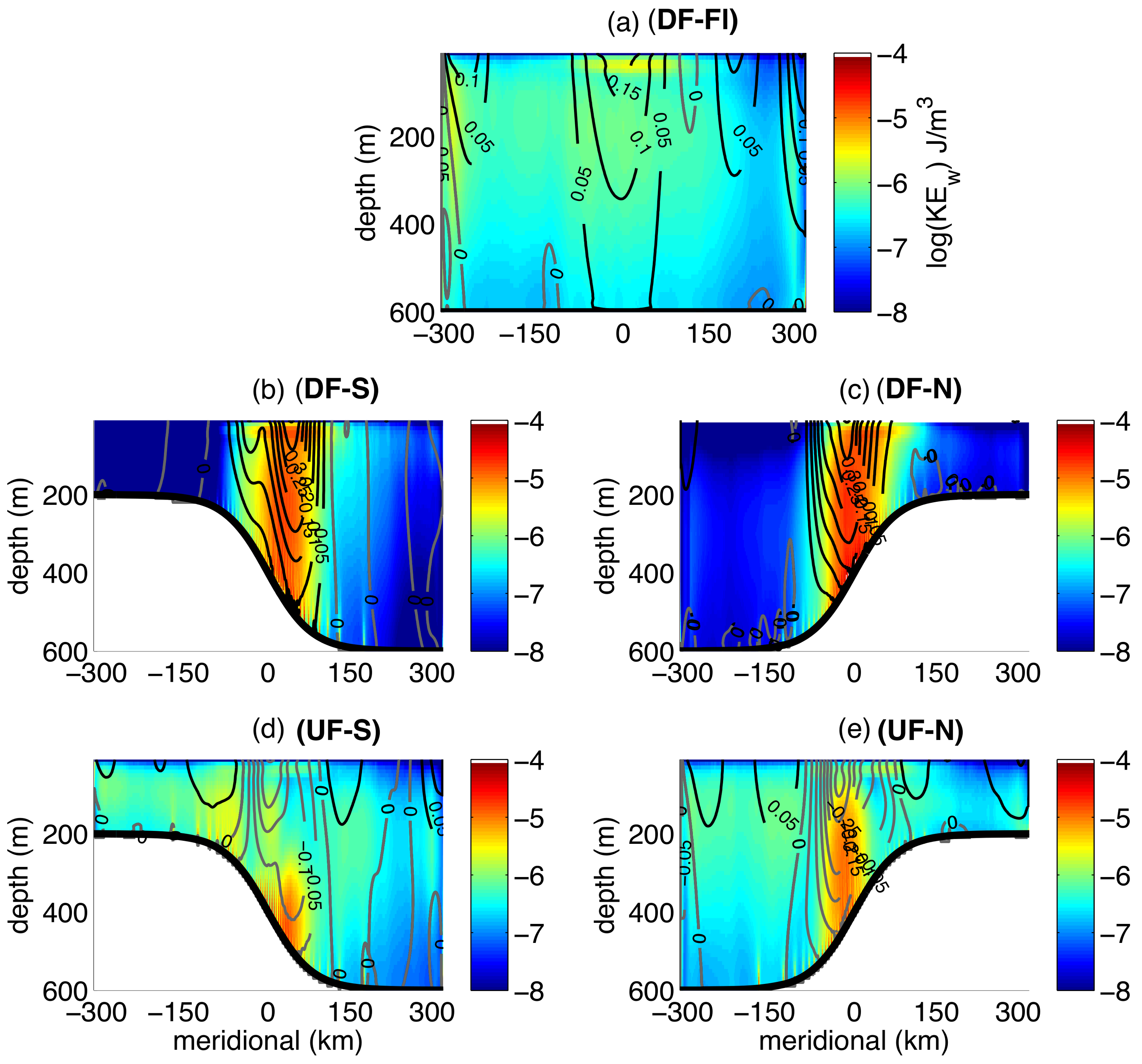
Fine spatial variability in the PV distributions also occurs near the bottom boundary. Figure 10 compares vertical kinetic energy as in all the simulations, where w is vertical velocity and is density. Here, frictional processes in the bottom boundary layer can, with a laterally-sheared mean flow, give rise to significant vertical velocities that influence the near-bottom stratification [52,53].
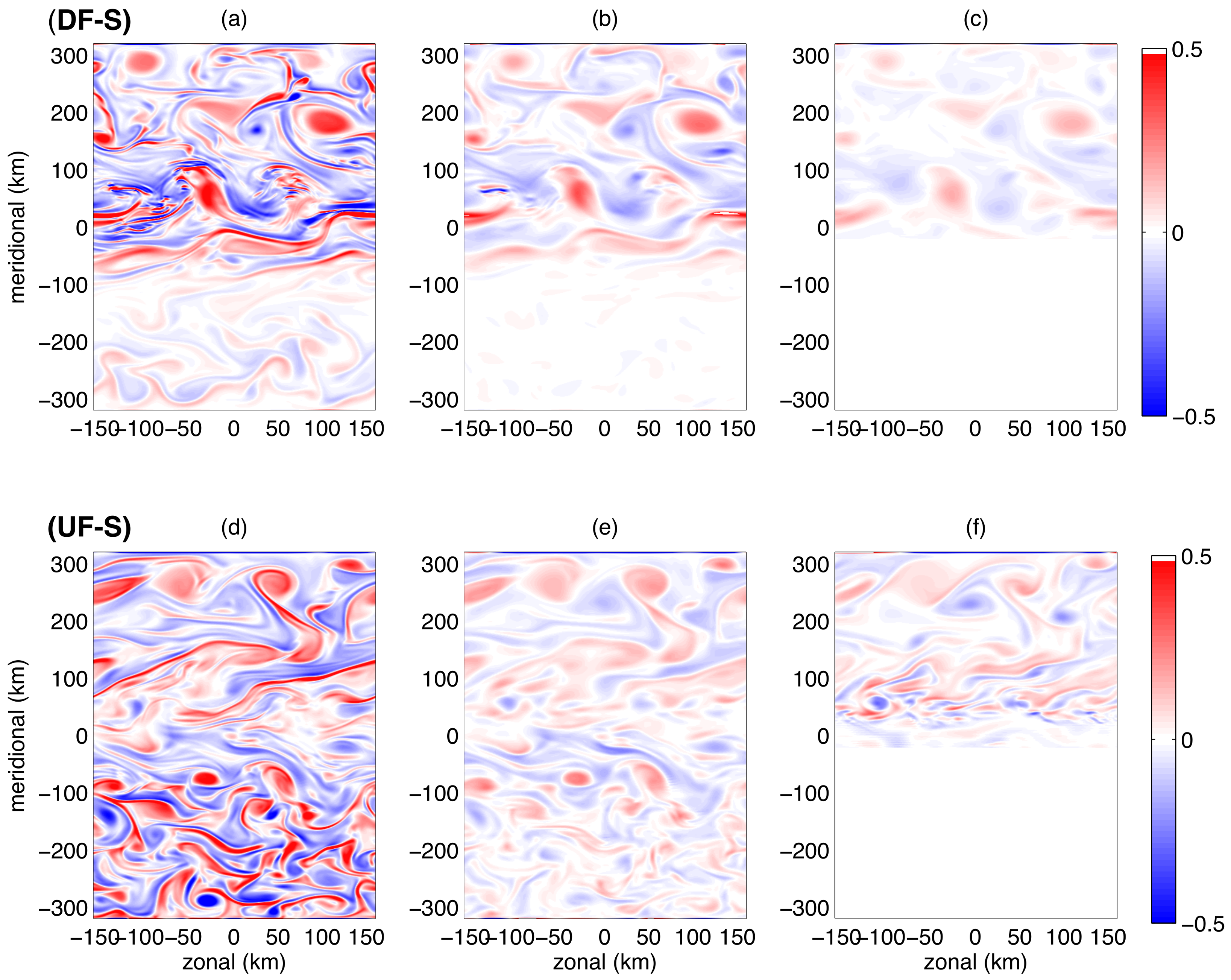
Over the continental slope, Ekman overturning acts as a PV sink in Experiment DF-N and UF-S, resulting in a low PV region. This region is associated with large vertical velocity and . We compare the vertical structures of for Experiment DF-S and UF-S in Figure 11. It is evident that in Experiment UF-S, Ekman overturning due to friction produces large at 300 m depth. close to the bathymetry is even larger than that at 150 m depth. In contrast, for Experiment DF-S, bottom friction is a source of PV, which inhibits the generation of large w or . In Figure 11a–c, decays in magnitude through the water column; there is no near-bottom enhancement.
In summary, the interaction of surface wind forcing, a strong mean flow and a topographic slope can lead to substantial changes in the interior PV over relatively short distances. These are reflected in the characteristics of the submesoscale motions, which are more active in low PV regions.
4.3. Interaction between Mesoscale and Submesoscale
Topography influences submesoscale motions primarily through mesoscale eddies. The interaction between the mesoscale and submesoscale motions can be studied through the correlation between submesoscale vertical velocities and mesoscale EKE [47]. Isachsen [17] has shown that eddy diffusivities in the ocean are sensitive to the ratio of topographic slope and isopycnal slope. In this study, all simulations with a topographic slope exhibit stronger isopycnal tilt than the flat-bottom control experiment, DF-Fl. However, the equilibrated EKE levels are spatially more complex, which is due to a tendency for a continental slope to dampen EKE levels. Over a steep continental slope, baroclinic instability is inhibited and EKE becomes smaller compared with a flat bottom experiment (Figure 9).
Comparing Figure 10 with Figure 9, we find that regions with enhanced submesoscale vertical velocities are also associated with larger mesoscale eddy kinetic energies. Similar to and the vertical velocities, EKE also shows an asymmetric distribution between the northern and southern flanks of the front, with larger values associated with weaker stratification. The only counter-intuitive case is Experiment DF-N, in which submesoscale motions are enhanced in the northern flank of the front but EKE is suppressed in the same region. The low EKE in the northern flank is mainly due to the isopycnal layers that interact with both the surface and the bathymetry (Figure 7). The transport of EKE from the frontal region to the northern flank is constrained by the isopycnal layers that outcrop on the continental slope and do not extend to the northern boundary. This results in a low EKE region coupled with a weak background PV and vertical stratification that still supports a shallow submesoscale field.
5. Conclusions
In this study, we examine the modulation of surface turbulence characteristics related to wind-induced frontal currents formed over a topographic slope. We link the surface properties to changes in interior PV distributions related to the orientation of the surface wind stress and the continental slope. Ekman transport over a topographic slope can generate low or high PV regions in the ocean interior, associated with weak or strong stratification near the surface, respectively. The presence of a topographic slope, and its suppression of mesoscale EKE, allows much steeper statistically-equilibrated isopycnal slopes that can give rise to deep m regions of weak vertical (and strong lateral) stratification. These conditions are conducive to a strong submesoscale velocity field. We find that this variability in the surface stratification generates meridional asymmetry in the kinetic energy spectra as well as the amplitude and skewness of the Rossby number. Variations in surface submesoscale turbulence by the topography is mainly through the modulation of mesoscale stirring, which is evident from the correlation between near-surface EKE and the amplitude of turbulent vertical velocities, but may also arise from changes in the near-surface reservoir of available potential energy. In addition to the modulation of surface turbulence, down-slope Ekman transport also generates a low PV region near the ocean floor and give rises to large vertical velocities near the ocean bottom.
The main conclusions of the study are summarized as follows:
- Surface vorticity characteristics are modified by the presence of a sloping bottom. Most of the persistent eddies near the surface are cyclonic.
- The sloping bottom modifies the spectra of near-surface vertical velocities and kinetic energies. Velocity spectra exhibit spatial asymmetries between the northern and southern flanks of the domain.
- Interaction of wind forcing, mean flow and a topographic slope can lead to substantial PV gradients over relatively short distances, which are generated by the Ekman transport at the sea surface and at the ocean bottom. These are reflected in the characteristics of the submesoscale motions, which are more active in low PV regions.
- Regions of enhanced submesoscale vertical velocity are associated with areas of larger mesoscale eddy kinetic energy due to enhanced stirring and the subsequent filamentation and frontogenesis associated with these larger-scale motions.
- These results are not consistent with the spectral predictions of SQG theory, which is perhaps not surprising due to strong interior PV gradients, but points to a critical role for ageostrophic velocities generated at both surface and bottom boundary layers.
These results suggest that along-slope wind stress and slope orientation exert substantial influence over the transport and mixing across the continental shelf. This has implications for the exchanges of mass, heat, salt, and biogeochemical tracers in coastal waters, and also for how they are parameterized in numerical simulations that have insufficient resolution to resolve these motions directly.
References
Author Contributions
Q.Z., A.F.T., and A.L. conceived and designed the experiments; Q.Z. performed the experiments; Q.Z., A.F.T., and A.L. analyzed the data; Q.Z., A.F.T., and A.L. wrote the paper.
Acknowledgments
We acknowledge assistance from Andrew Stewart in configuring the numerical simulations as well as helpful conversations from Xiaozhou Ruan and Mar Flexas. A.F.T. was supported by National Science Foundation (NSF) grant OPP-1246460; A.L. was supported by NSF grant OCE-1235488.
Conflicts of Interest
The authors declare no conflict of interest. The funding sponsors had no role in the design of the study; in the collection, analyses, or interpretation of data; in the writing of the manuscript, and in the decision to publish the results.
References
- Thomas, L.N.; Tandon, A.; Mahadevan, A. Submesoscale processes and dynamics. Ocean Model. Eddying Regime Geophys. Monogr. Ser. 2008, 177, 17–38. [Google Scholar]
- Klein, P.; Lapeyre, G. The oceanic vertical pump induced by mesoscale and submesoscale turbulence. Ann. Rev. Mar. Sci. 2009, 1, 351–375. [Google Scholar] [CrossRef] [PubMed]
- Klein, P.; Hua, B.L.; Lapeyre, G.; Capet, X.; Le Gentil, S.; Sasaki, H. Upper ocean turbulence from high-resolution 3D simulations. J. Phys. Oceanogr. 2008, 38, 1748–1763. [Google Scholar] [CrossRef]
- Mahadevan, A.; Archer, D. Modeling the impact of fronts and mesoscale circulation on the nutrient supply and biogeochemistry of the upper ocean. J. Geophys. Res. 2000, 105, 1209–1225. [Google Scholar] [CrossRef]
- Levy, M.; Ferrari, R.; Franks, P.J.S.; Martin, A.P.; Riviere, P. Bringing physics to life at the submesoscale. Geophys. Res. Lett. 2012, 39. [Google Scholar] [CrossRef] [Green Version]
- Omand, M.M.; D’Asaro, E.A.; Lee, C.M.; Perry, M.J.; Briggs, N.; Cetinic, I.; Mahadevan, A. Eddy-driven subduction exports particulate organic carbon from the spring bloom. Science 2015, 348, 222–225. [Google Scholar] [CrossRef] [PubMed]
- Fox-Kemper, B.; Ferrari, R.; Hallberg, R. Parameterization of mixed layer eddies. Part I: Theory and diagnosis. J. Phys. Oceanogr. 2008, 38, 1145–1165. [Google Scholar] [CrossRef]
- Siegel, A.; Weiss, J.B.; Toomre, J.; McWilliams, J.C.; Berloff, P.S.; Yavneh, I. Eddies and vortices in ocean basin dynamics. Geophys. Res. Lett. 2001, 28, 3183–3186. [Google Scholar] [CrossRef]
- Mensa, J.A.; Garraffo, Z.; Griffa, A.; Ozgokmen, T.M.; Haza, A.; Veneziani, M. Seasonality of the submesoscale dynamics in the Gulf Stream region. Ocean Dyn. 2013, 63, 923–941. [Google Scholar] [CrossRef]
- Sasaki, H.; Klein, P.; Qiu, B.; Sasai, Y. Impact of oceanic-scale interactions on the seasonal modulation of ocean dynamics by the atmosphere. Nat. Commun. 2014, 5. [Google Scholar] [CrossRef] [PubMed]
- Boccaletti, G.; Ferrari, R.; Fox-Kemper, B. Mixed layer instabilities and restratification. J. Phys. Oceanogr. 2007, 37, 2228–2250. [Google Scholar] [CrossRef]
- Capet, X.; Mcwilliams, J.C.; Mokemaker, M.J.; Shchepetkin, A.F. Mesoscale to submesoscale transition in the California current system. Part I: Flow structure, eddy flux, and observational tests. J. Phys. Oceanogr. 2008, 38, 29–43. [Google Scholar] [CrossRef]
- Su, Z.; Wang, J.; Klein, P.; Thompson, A.; Menemenlis, D. Ocean submesoscales as a key component of the global heat budget. Nat. Commun. 2018, 9, 775. [Google Scholar] [CrossRef] [PubMed]
- Hart, J.E. Baroclinic Instability over a Slope. 1. Linear Theory. J. Phys. Oceanogr. 1975, 5, 625–633. [Google Scholar] [CrossRef]
- Poulin, F.J.; Flierl, G.R. The influence of topography on the stability of jets. J. Phys. Oceanogr. 2005, 35, 811–825. [Google Scholar] [CrossRef]
- Thompson, A.F. Jet formation and evolution in baroclinic turbulence with simple topography. J. Phys. Oceanogr. 2010, 40, 257–278. [Google Scholar] [CrossRef]
- Isachsen, P.E. Baroclinic instability and eddy tracer transport across sloping bottom topography: How well does a modified Eady model do in primitive equation simulations? Ocean Model. 2011, 39, 183–199. [Google Scholar] [CrossRef]
- Stewart, A.; Thompson, A. The temporal residual mean overturning circulation in neutral density coordinates. Ocean Model. 2015, 90, 44–56. [Google Scholar] [CrossRef]
- Stern, A.; Nadeau, L.P.; Holland, D. Instability and mixing of zonal jets along an idealized continental shelf break. J. Phys. Oceanogr. 2015, 45, 2315–2338. [Google Scholar] [CrossRef]
- Wang, D.P.; Jordi, A. Surface frontogenesis and thermohaline intrusion in a shelfbreak front. Ocean Model. 2011, 38, 161–170. [Google Scholar] [CrossRef]
- Spall, M.A. Dense water formation around islands. J. Geophys. Res. 2013, 118, 2507–2519. [Google Scholar] [CrossRef]
- Thompson, A.F.; Heywood, K.J. Frontal structure and transport in the northwestern Weddell Sea. Deep Sea Res. I 2008, 55, 1229–1251. [Google Scholar] [CrossRef]
- Thompson, A.F.; Heywood, K.J.; Schmidtko, S.; Stewart, A.L. Eddy transport as a key component of the Antarctic overturning circulation. Nat. Geosci. 2014, 7, 879–884. [Google Scholar] [CrossRef]
- Stewart, A.L.; Thompson, A.F. Connecting antarctic cross-slope exchange with southern ocean overturning. J. Phys. Oceanogr. 2013, 43, 1453–1471. [Google Scholar] [CrossRef]
- D’Asaro, E.; Lee, C.; Rainville, L.; Harcourt, R.; Thomas, L. Enhanced turbulence and energy dissipation at ocean fronts. Science 2011, 332, 318–322. [Google Scholar] [CrossRef] [PubMed]
- Shcherbina, A.Y.; D’Asaro, E.A.; Lee, C.M.; Klymak, J.M.; Molemaker, M.J.; McWilliams, J.C. Statistics of vertical vorticity, divergence, and strain in a developed submesoscale turbulence field. Geophys. Res. Lett. 2013, 40, 4706–4711. [Google Scholar] [CrossRef]
- Thomas, L.N.; Taylor, J.R.; Ferrari, R.; Joyce, T.M. Symmetric instability in the Gulf Stream. Deep Sea Res. II 2013, 91, 96–110. [Google Scholar] [CrossRef]
- Thompson, A.; Lazar, A.; Buckingham, C.; Garabato, A.N.; Damerell, G.; Heywood, K. Open-ocean submesoscale motions: A full seasonal cycle of mixed layer instabilities from gliders. J. Phys. Oceanogr. 2016, 46, 1285–1307. [Google Scholar] [CrossRef]
- Gula, J.; Molemaker, M.J.; McWilliams, J.C. Topographic generation of submesoscale centrifugal instability and energy dissipation. Nat. Commun. 2016, 7, 12811. [Google Scholar] [CrossRef] [PubMed]
- Ruan, X.; Thompson, A.F.; Flexas, M.M.; Sprintall, J. Contribution of topographically generated submesoscale turbulence to Southern Ocean overturning. Nat. Geosci. 2017, 10, 840–845. [Google Scholar] [CrossRef]
- Kloosterziel, R.C.; Carnevale, G.F.; Orlandi, P. Inertial instability in rotating and stratified fluids: Barotropic vortices. J. Fluid Mech. 2007, 583, 379–412. [Google Scholar] [CrossRef]
- Lazar, A.; Stegner, A.; Heifetz, E. Inertial instability of intense stratified anticyclones. Part 1. Generalized stability criterion. J. Fluid Mech. 2013, 732, 457–484. [Google Scholar] [CrossRef] [Green Version]
- Afanasyev, Y.D.; Peltier, W.R. Three-dimensional instability of anticyclonic swirling flow in rotating fluid: Laboratory experiments and related theoretical predictions. Phys. Fluids 1998, 10, 3194–3202. [Google Scholar] [CrossRef]
- Lazar, A.; Stegner, A.; Caldeira, R.; Dong, C.; Didelle, H.; Viboud, S. Inertial instability of intense stratified anticyclones. Part 2. Laboratory experiments. J. Fluid Mech. 2013, 732, 485–509. [Google Scholar] [CrossRef]
- Munk, W.; Armi, L.; Fischer, K.; Zachariasen, F. Spirals on the sea. Proc. R. Soc. Lond. A 2000, 456, 1217–1280. [Google Scholar] [CrossRef]
- Eldevik, T.; Dysthe, K.B. Spiral eddies. J. Phys. Oceanogr. 2002, 32, 851–869. [Google Scholar] [CrossRef]
- Buckingham, C.; Garabato, A.N.; Thompson, A.; Brannigan, L.; Lazar, A.; Marshall, D.; Nurser, A.; Damerell, G.; Heywood, K.; Belcher, S. Seasonality of submesoscale flows in the ocean surface boundary layer. Geophys. Res. Lett. 2016, 43, 2118–2126. [Google Scholar] [CrossRef] [Green Version]
- Thomas, L.N. Destruction of potential vorticity by winds. J. Phys. Oceanogr. 2005, 35, 2457–2466. [Google Scholar] [CrossRef]
- Hoskins, B.J. The Mathematical-Theory of Frontogenesis. Ann. Rev. Fluid Mech. 1982, 14, 131–151. [Google Scholar] [CrossRef]
- Benthuysen, J.; Thomas, L.N. Friction and Diapycnal Mixing at a Slope: Boundary Control of Potential Vorticity. J. Phys. Oceanogr. 2012, 42, 1509–1523. [Google Scholar] [CrossRef]
- Marshall, J.; Radko, T. Residual-mean solutions for the Antarctic Circumpolar Current and its associated overturning circulation. J. Phys. Oceanogr. 2003, 33, 2341–2354. [Google Scholar] [CrossRef]
- Marshall, J.; Speer, K. Closure of the meridional overturning circulation through Southern Ocean upwelling. Nat. Geosci. 2012, 5, 171–180. [Google Scholar] [CrossRef]
- Large, W.G.; Danabasoglu, G.; Doney, S.C.; McWilliams, J.C. Sensitivity to surface forcing and boundary layer mixing in a global ocean model: Annual-mean climatology. J. Phys. Oceanogr. 1997, 27, 2418–2447. [Google Scholar] [CrossRef]
- Poulin, F.J.; Stegner, A.; Hernández-Arencibia, M.; Marrero-Díaz, A.; Sangrà, P. Steep Shelf Stabilization of the Coastal Bransfield Current: Linear Stability Analysis. J. Phys. Oceanogr. 2014, 44, 714–732. [Google Scholar] [CrossRef]
- Cimoli, L.; Stegner, A.; Roullet, G. Meanders and eddies formation by a buoyant coastal current flowing over a sloping topography. Ocean Sci. Discuss. 2017, 13, 905–923. [Google Scholar] [CrossRef]
- Callies, J.; Ferrari, R. Interpreting Energy and Tracer Spectra of Upper-Ocean Turbulence in the Submesoscale Range (1–200 km). J. Phys. Oceanogr. 2013, 43, 2456–2474. [Google Scholar] [CrossRef]
- Rosso, I.; Hogg, A.M.; Kiss, A.E.; Gayen, B. Topographic influence on submesoscale dynamics in the Southern Ocean. Geophys. Res. Lett. 2015, 42, 1139–1147. [Google Scholar] [CrossRef]
- Mahadevan, A.; Tandon, A.; Ferrari, R. Rapid changes in mixed layer stratification driven by submesoscale instabilities and winds. J. Geophys. Res. 2010, 115. [Google Scholar] [CrossRef]
- Hoskins, B.J. The role of potential vorticity in symmetric stability and instability. Q. J. R. Meteorol. Soc. 1974, 100, 480–482. [Google Scholar] [CrossRef]
- Tayor, J.; Ferrari, R. On the equilibration of a symmetrically unstable front via a secondary shear instability. J. Fluid Mech. 2009, 622, 103–113. [Google Scholar]
- Bachman, S.; Taylor, J. Modelling of partially-resolved oceanic symmetric instability. Ocean Model. 2014, 82, 15–27. [Google Scholar] [CrossRef]
- Benthuysen, J.A.; Thomas, L.N. Nonlinear stratified spindown over a slope. J. Fluid Mech. 2013, 726, 371–403. [Google Scholar] [CrossRef]
- Ruan, X.; Thompson, A. Bottom boundary potential vorticity injection from an oscillating flow: A PV pump. J. Phys. Oceanogr. 2016, 46, 3509–3526. [Google Scholar] [CrossRef]
Figure 1.
(a) Overview map of the Weddell Sea sector of the Southern Ocean. (b) An enhanced view of the red box in panel (a), where bathymetry (m) is given in color. Circles in panel (b) correspond to a single hydrographic transect collected by an ocean glider in January 2012. (c) Vertical, cross-slope section of cross-transect (along-slope) velocity, v; the zero contour is given in white. (d) Rossby number approximated by , where x is the cross-slope direction of the same transect in panel (c). Tick marks at the top of panel (c) indicate the surfacing positions of each glider dive. See Thompson et al. [23] for further details.

Figure 2.
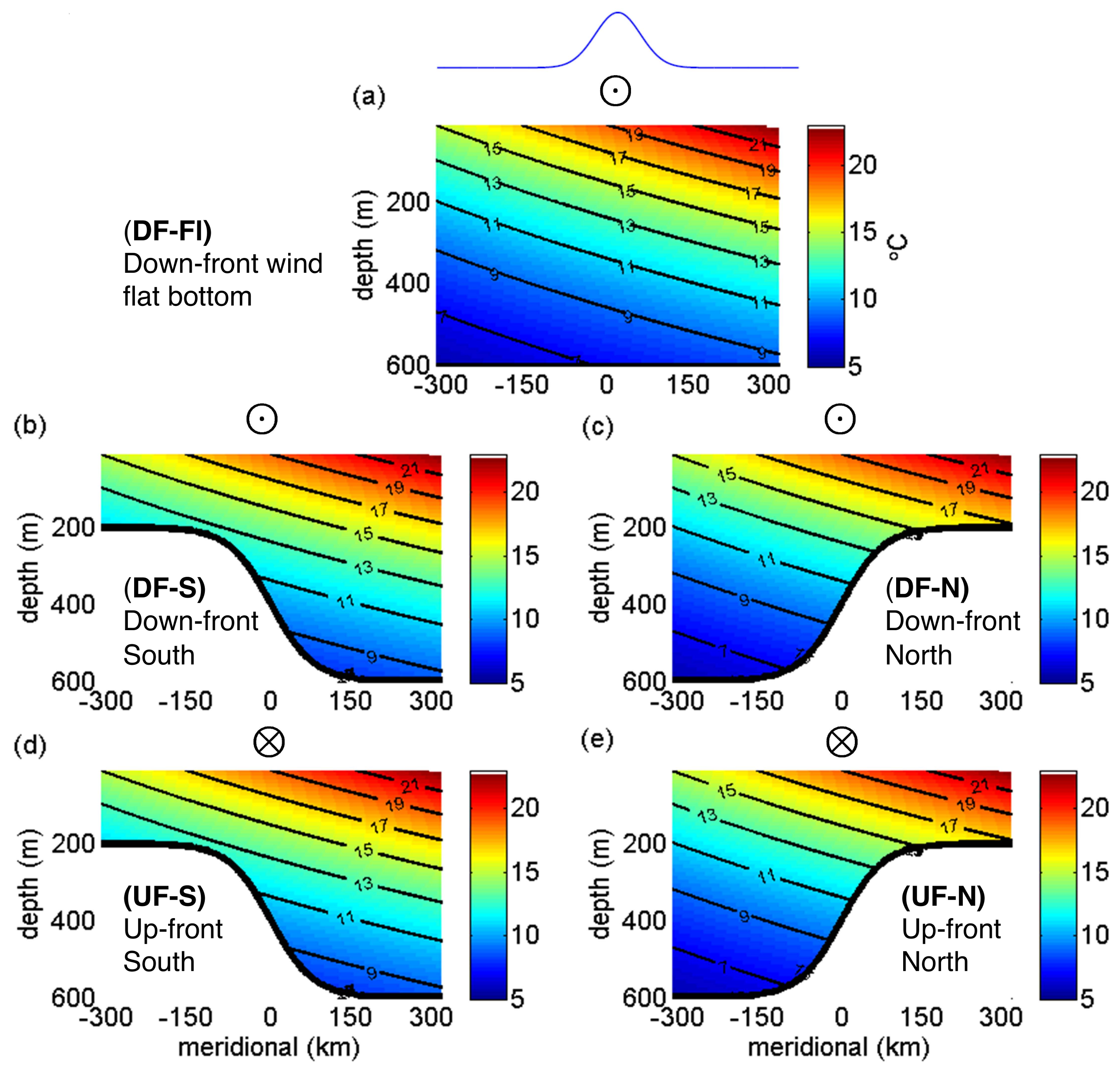
Schematic overview of the model configuration for the five simulations described in Table 1. Panels (a–e) correspond to experiments (1)–(5). Experiment ID is indicated in each panel. Colors and contours show the zonally-uniform initial temperature profile. The temperature is relaxed to these initial values at the northern and southern boundaries. The thick black curve marks the bathymetry, while the circle over each panel marks the wind orientation: down-front (dots) or up-front (crosses). The blue curve on the top of panel (a) shows the surface wind stress profile, with a peak value N m−2.
Figure 2.
Schematic overview of the model configuration for the five simulations described in Table 1. Panels (a–e) correspond to experiments (1)–(5). Experiment ID is indicated in each panel. Colors and contours show the zonally-uniform initial temperature profile. The temperature is relaxed to these initial values at the northern and southern boundaries. The thick black curve marks the bathymetry, while the circle over each panel marks the wind orientation: down-front (dots) or up-front (crosses). The blue curve on the top of panel (a) shows the surface wind stress profile, with a peak value N m−2.

Figure 3.
(a) Growth of total kinetic energy in Experiment DF-S. (b) Snapshots at day 900 for Experiment DF-S (Table 1) surface potential temperature (°C) at 10 m depth. (c) Same as (b), for vertical velocity w ( m s−1) at 30 m depth.
Figure 3.
(a) Growth of total kinetic energy in Experiment DF-S. (b) Snapshots at day 900 for Experiment DF-S (Table 1) surface potential temperature (°C) at 10 m depth. (c) Same as (b), for vertical velocity w ( m s−1) at 30 m depth.

Figure 4.
Near-surface Rossby number, , at 10 m depth for the five experiments. Panels (a–e) correspond to experiments (1)–(5) described in Table 1, and experiment ID is indicated. The left-hand plot in each plan shows the zonally-averaged root mean square (RMS) averaged over a period of 200 days. The right-hand plot is a snapshot of surface at day 900.

Figure 5.
Spectra of surface horizontal kinetic energy (10 m depth, left panels) and vertical velocity (30 m depth, right panels) averaged from day 800 to 1000. (a) Kinetic energy spectra and (b) vertical velocity spectra in Experiment DF-Fl. (c) Kinetic energy spectra and (d) vertical velocity spectra in Experiment DF-S. (e) Kinetic energy spectra and (f) vertical velocity spectra in Experiment DF-N. Dotted lines represent and spectral slope, provided for reference. Blue lines represent the southern flank of the domain from −300 km −100 km. Red lines represent the middle of the domain (frontal region) from −100 km 100 km. Black lines represent the northern flank of the domain from 100 km 300 km. Spectra in Experiments UF-S and UF-N are similar to those in the control Experiment DF-Fl, and are not shown in this figure.

Figure 6.
Probability density function (PDF) for (a) surface Rossby number, and (b) Rossby number at 180 m depth averaged from day 800 to 1000 for Experiments (1)–(5). Values of PDF skewness are labeled using the same color for each experiment.
Figure 6.
Probability density function (PDF) for (a) surface Rossby number, and (b) Rossby number at 180 m depth averaged from day 800 to 1000 for Experiments (1)–(5). Values of PDF skewness are labeled using the same color for each experiment.

Figure 7.
PV cross section in the middle of the domain (x = 0) averaged from day 800 to 1000. Values are displayed in scale. Black contours show the mean potential temperature and also indicate isopycnal surfaces. Panels (a–e) correspond to experiments (1)–(5) described in Table 1, and experiment ID is indicated.

Figure 8.
Upper panels are PV snapshots on the 12 °C (a), 14 °C (b), and 18 °C (c) isopycnal surfaces at day 900 for Experiment DF-S. White areas indicate the isopycnal surface intersecting with the topographic slope or the surface. Lower panels (d–f) are the corresponding time and zonal averaged PV fluxes. PV fluxes are calculated using snapshots between day 800 and 1000.

Figure 9.
Zonal and time averaged EKE () from day 800 to 1000. Values are displayed in scale. Contour lines show zonal and time averaged zonal velocity (u). Black line represents positive values. Gray line represents negative values. Panels (a–e) correspond to experiments (1)–(5) described in Table 1, and experiment ID is indicated.

Figure 10.
Zonal and time averaged vertical kinetic energy () from day 800 to 1000 for for five experiments. Values are displayed in scale. Contour lines show zonal and time averaged zonal velocity (u). Black line represents positive values. Gray line represents negative values. Panels (a–e) correspond to experiments (1)–(5) described in Table 1, and experiment ID is indicated.

Figure 11.
Vertical structure of at day 900 for Experiment DF-S (a–c) and Experiment UF-S (d–f). Cross sections at 10 m, 150 m, and 300 m depth are shown. White areas in (c,f) are associated with topographic slope interception.
Figure 11.
Vertical structure of at day 900 for Experiment DF-S (a–c) and Experiment UF-S (d–f). Cross sections at 10 m, 150 m, and 300 m depth are shown. White areas in (c,f) are associated with topographic slope interception.


Table 1.
Simulation configurations. The five experiments correspond to the schematics in Figure 2. The identifying characteristics include the wind and topography orientation. The front velocity is diagnosed at the location where is greatest, when the simulation has reached a statistically-equilibrated state.
| Experiment Number | Experiment ID | Surface Wind Orientation | Shelf Location | Frontal Zonal Velocity (m s−1) |
|---|---|---|---|---|
| 1 | DF-Fl | down-front | flat bottom | 0.1895 |
| 2 | DF-S | down-front | south | 0.4047 |
| 3 | DF-N | down-front | north | 0.4086 |
| 4 | UF-S | up-front | south | −0.2589 |
| 5 | UF-N | up-front | north | −0.3694 |
© 2018 by the authors. Licensee MDPI, Basel, Switzerland. This article is an open access article distributed under the terms and conditions of the Creative Commons Attribution (CC BY) license (http://creativecommons.org/licenses/by/4.0/).
Share and Cite
MDPI and ACS Style
Lazar, A.; Zhang, Q.; Thompson, A.F. Submesoscale Turbulence over a Topographic Slope. Fluids 2018, 3, 32. https://doi.org/10.3390/fluids3020032
AMA Style
Lazar A, Zhang Q, Thompson AF. Submesoscale Turbulence over a Topographic Slope. Fluids. 2018; 3(2):32. https://doi.org/10.3390/fluids3020032
Chicago/Turabian StyleLazar, Ayah, Qiong Zhang, and Andrew F. Thompson. 2018. "Submesoscale Turbulence over a Topographic Slope" Fluids 3, no. 2: 32. https://doi.org/10.3390/fluids3020032