Electrorheological Model Based on Liquid Crystals Membranes with Applications to Outer Hair Cells

Abstract

Liquid crystal flexoelectric actuation uses an imposed electric field to create membrane bending, this phenomenon is found in outer hair cells (OHC) located in the inner ear, whose role is to amplify sound through the generation of mechanical power. Oscillations in the OHC membranes create periodic viscoelastic flows in the contacting fluid media. A key objective of this work on flexoelectric actuation relevant to OHC is to find the relations and impact of the electro-mechanical properties of the membrane, the rheological properties of the viscoelastic media, and the frequency response of the generated mechanical power output. The model developed and used in this work is based on the integration of: (i) the flexoelectric membrane shape equation applied to a circular membrane attached to the inner surface of a circular capillary, and (ii) the coupled capillary flow of contacting viscoelastic phases, which are characterized by the Jeffreys constitutive equation with different material conditions. The membrane flexoelectric oscillations drive periodic viscoelastic capillary flows, as in OHCs. By applying the Fourier transform formalism to the governing equations and assuming small Mach numbers, analytical equations for the transfer function, associated to the average curvature, and for the volumetric rate flow as a function of the electrical field were found, and these equations can be expressed as a third-order differential equation which depends on the material properties of the system. When the inertial mechanisms are considered, the power spectrum shows several resonance peaks in the average membrane curvature and volumetric flow rate. When the inertia is neglected, the system follows a non-monotonic behavior in the power spectrum. This behavior is associated with the solvent contributions related to the retardation-Jeffreys mechanisms. The specific membrane-viscoelastic fluid properties that control the power response spectrum are identified. The present theory, model, and computations contribute to the evolving fundamental understanding of biological shape actuation through electromechanical couplings.

1. Introduction

Liquid crystals are multifunctional materials which form part of many biological material processes, such as sensor and actuator devices, natural super fibers, membranes, films, and drops [1,2,3]. Other remarkable properties, such as film formation and surface pattern, can be found in biological plywoods, beetles’ cuticle [1,2,3,4], and cholesteric film formation flows of collagen solutions [3,4]. This paper presents the theory and simulation of a physiological actuator device whose functioning hinges on unique electro-mechanical properties of mesophases and is a prototypical example of responsive self-organizing materials [1,2,5,6,7,8,9].

The functioning of outer hair cells (OHC) in the inner ear involves electric-field driven periodic curvature oscillations of liquid crystal (LC) elastic membranes that impart, by bending and oscillating [9], momentum and flow to the contacting bulk viscoelastic fluids [10]. This important phenomenon has been studied with several mechanical and mathematical modelling approaches using different constitutive equations [11,12,13,14,15,16,17]. The electric field actuation of the liquid crystal membrane is known as flexoelectricity [7,8,9] and it was studied and developed by Petrov and co-workers [6,7,8]. The key role of OHC is sound amplification in the presence of bulk viscous dissipation and energy storage in the elastic flexoelectric membrane [10,11,12,13,14]. Hence, the full description and understanding of OHC functioning has to include the frequency response of flexoelectric membranes embedded in viscous and viscoelastic media due to an oscillating electric E field [11,15]. The input oscillating E field, through the electromechanical flexoelectric effect, produces curvature oscillations in the elastic membrane that comprises the OHC surrounded by viscoelastic media [9,10,15]. In turn, the oscillating elastic membrane displaces the contacting viscoelastic liquids through the mechanical visco-elastic and dissipation mechanisms [10,15]. The combined effect that allows the electro-mechanical energy conversion is based on the integration of the flexoelectric effect (E field imposed on flexoelectric membrane) and the mechanical effect (membrane elasticity plus viscoelastic bulk fluid flow) [10,15].

A great deal of analytical approaches have been employed in order to simulate the changes in the average membrane curvature of a flexoelectric membrane as a function of the electrical field [9,10,11,12,13]. Ricently Aguilar-Gutierrez et al. [14], studied the curvature dissipation for liquid surfaces and mebranes from a generalized Boussiness-Scriven surface approach [14]. Rabbits et al. [15] developed a model based on a mixture-composite constitutive model. Their results show that the peak power efficiency is likely tunned to a specific frequency that depends on OHC length. Moreover, this tuning may contribute to the frequency selectivity of the cochlea [15]. Other appraoches have employed electromecanical models with focus on hearing, composite membranes and isolated cochlear outer hair cells [16,17,18]. From a mechanical-transduction point of view, some researchers have used voltage and tension-dependent mathematical models to describe lipid mobility in the outer hair cell plasma membrane, bending models with emphasis in cell electromotility, and genetics of the auditory hair cells [19,20,21]. Some other electromechanical and rheological models have been proposed, which include electromagnetic mechanisms, the viscoelastic-relaxation dynamical response of the curvature through different rheological tests, including oscillatory and creep flow [22,23,24]. From an electromechanical point of view, the reverse transduction, negative membrane capacitance, frequency response, and resonance curvature of these physical models [25,26,27,28], play an important role in the audition mechanisms of the cochlea and the energy output from the outer hair cells [25,26,27,28]. Other authors have focused in the description of the mammalian cochlear hair cells through power generation [29], splay, energy, current noise spectrum, viscous fluid loss mechanisms, noise spectrum, stress of the membrane capacitance, and hair bundle motility [30,31,32,33].

In this context, we have developed several mathematical approaches to describe the flexoelectric membrane curvature through liquid crystal theory [1,2,3,6,7,8] and electrorheological models with emphasis in Outer Hair Cells (OHC) device modeling [9,10,11,12,13,14].

We would like to emphasize that “one of the main issues in this area is to find the monotonically and non-monotonic power dissipation in the system” induced by the changes in the curvature as a consequence of the imposed electrical field [10,12]; this power dissipation is characterized by a spectrum that depends on the electric field frequency and its specific features, such as resonant and antiresonance peaks, are the key issue of this this paper [10,12].

In order to include the physical nature of the fluids, several constitutive equations have been employed [9,10,11,12,13,14], from Euler (inviscid fluid) [9] to Maxwell constitutive equations [10], which have led to the governing ordinary differential equations that describe the changes in the curvature as a function of the electrical field [9,10,11,12]. Depending on the rheological equation of state, the shape of the power resonance can display several resonance curves in the regime of small inertia [12] and zero inertia (Deborah number equal to zero) [10,12]. These resonance curves can be described in terms of linear ordinary differential equations, whose order (n) is defined by the total viscosity operator in the system [10,12]. For example, in the case of Euler and Newton fluids (n = 0), the power dissipation in the contacting bulk phases does not show resonance behavior [9], but when the physical nature of the fluids is viscoelastic (Maxwell, n = 2), the system shows a resonance behavior as a function of the frequency [10,12].

The originality of this research consists of a critical and significant generalization of the above-mentioned works, including:

(a)

The mathematical formulation developed here can be applied for any linear viscoelastic constitutive equation including fracctional linear operators;

(b)

The viscosity operator choosen to characterize the rheology and the transfer momentum of the membrane into the viscoelastic liquid phases is the sum of a solvent and polymer contributions. When the solvent viscosities are zero, the system reduces to a previous model recently published [9,14]; and

(c)

The effects of the solvent and polymer mechanisms induce a resonance and anti-resonance behavior (maximum and minimum), and the order of the electro-rheological model is three, whereas when the order of the dynamical equation is even, the system does not show a non-monotonic behavior. This new odd-even effect narrows down possible models from the outset.

In general, the shape of the power resonance as well as the monotonical and non-monotonical behavior depend on the order of the ODE that describes the average membrane curvature as a function of the applied electrical field and the Deborah number [14], which can be more properly interpreted as a reduced Mach number associated with the membrane speed propagation in the viscoelastic media. From extensive analysis based on an increasing order in classical viscoelastic models, it is found that: (i) for zero Mach numbers the power shows resonance behavior in the classical viscoelastic models (Maxwell, Jeffrey’s, and Burger’s models), meanwhile the non-monotonical behavior is displayed in the Jeffrey’s model (3ODE); (ii) when the inertia is included Ma ≠ 0, the system shows several resonance peaks, while at Ma >> 1 the system does not show any resonance peak at all. These generic findings narrow the range of relevant rheological conditions and rheological models, and allows us to establish connections between device output and material properties [9,10,11,12,13,14].

The three key issues to address in this energy conversion device are:

(i)

The magnitude of the power P associated with the average curvature or volumetric rate flow delivered to the contacting of viscoelastic Jeffrey’s fluids from the imposed oscillating electric field E;

(ii)

The minimum complexity of the Non-Newtonian model necessary to give the non-monotonically behavior in the power spectrum; and

(iii)

The necessary material conditions to have a well-localized maximum and minimum resonant power peak (in the spectrum of power dissipation) as physiologically required [25,32].

As a partial summary, both the direct and converse membrane flexoelectric effects are sensor-actuator properties when membrane curvature and polarization are coupled as in nematic liquid crystals [1,2,3,6,7,8]. Membrane flexoelectricity due to its inherent sensor-actuator capabilities is an area of current interest in medicine, soft matter and biological materials [33,34,35,36,37,38].

The specific objectives of this paper are:

(1)

Deriving a third-order dynamic linear model for a flexoelectric membrane attached to a capillary tube that contains Jeffrey’s viscoelastic fluids and is subjected to a fluctuating small amplitude electric field of arbitrary frequency.

(2)

Computing the frequency response of the electrorheological device taking into account the viscoelastic nature of the contacting fluids;

(3)

Using the modeling results to characterize the non-monotonic power spectrum associated to the role of membrane flexo-electricity and contacting fluid viscoelasticity of the device; and

(4)

Identifying the material properties that lead to electromechanical conversion relevant to functioning of OHC.

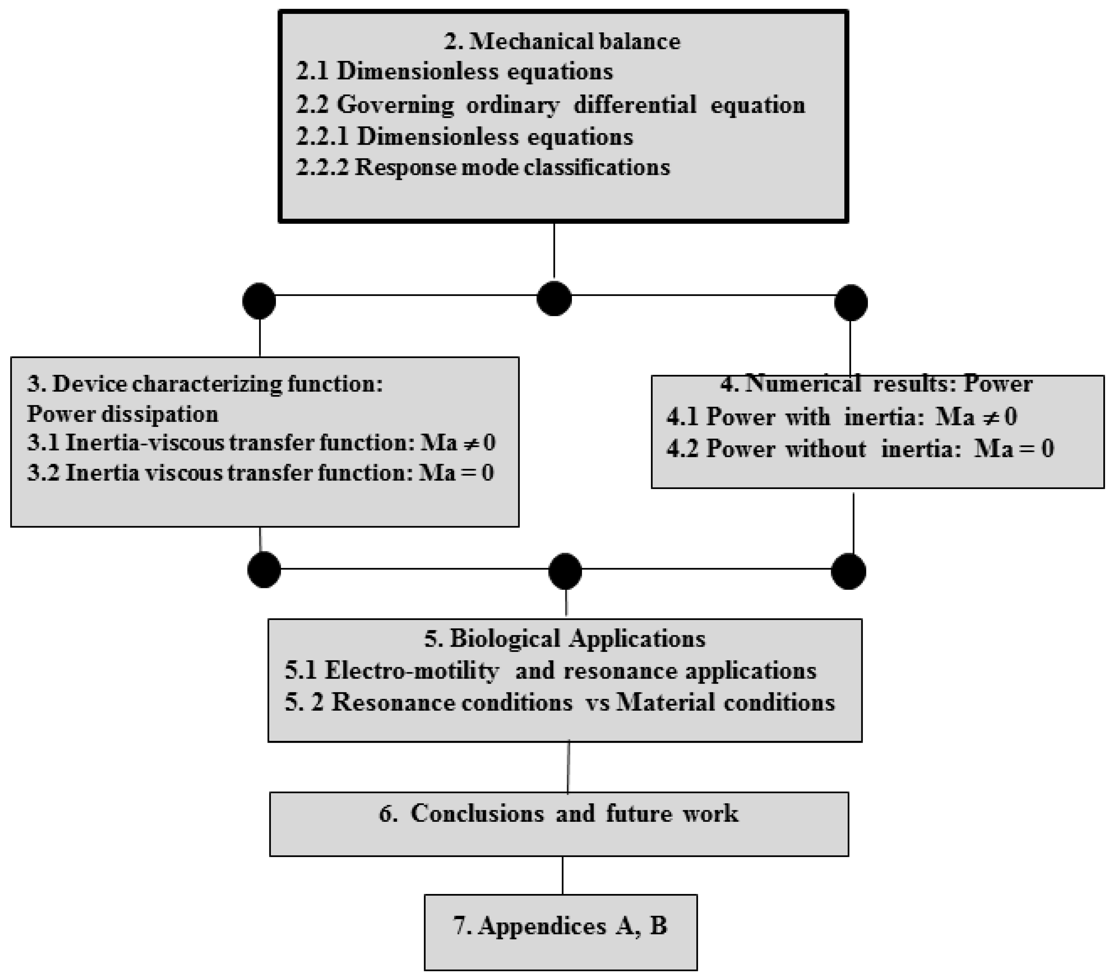
To avoid repetition of lengthy derivations the reader is referred to [10,12]. In [10] we describe the fluid viscoelasticity with a Maxwell fluid model, neglect momentum inertia (zero Deborah number: De = 0), and formulate the model in the time domain. In [12] we extend the previous Maxwell model with the inertial mechanisms (Deborah number: De ≠ 0) and using the Fourier formalism two power resonance power peaks were found [12] (see Appendices of ref. [12]). These two early works do not show a minimum in the power spectrum [10,12], such as other mathematical approaches [15]. In this research, we model the system in the frequency domain, including momentum inertia, and develop a generic approach that can be used in the future with any linear and fractional viscoelastic constitutive equation, as required by experimental results [15]. The new approach is novel and significant because we extend the power spectrum with a well localized maximum and minimum, i.e., a non-monotonically behavior found in biological systems such as outer hair cell [15] (see Figure 7 of ref. [15]). This paper is organized as shown in Figure 1. Section 2 introduces the generic features of the dimensionless governing electro-rheological model of the electric field responsive membrane embedded in Jeffrey’s viscoelastic fluids. Dimensionless numbers and characteristic modes. The governing equation is based on the integration of: (i) the flexoelectric membrane shape equation applied to a circular membrane attached to the inner surface of a circular capillary; and (ii) the capillary flow of the contacting viscoelastic phases. Section 3 presents the characteristic spectrum of the power output as a function of the Mach number and dimensionless numbers associated to the flexo-electric, viscoelastic and elastic mechanisms of the system. Section 4 presents selected representative numerical results of the device (small and zero Mach numerical values). Section 5 deals with the discussion of the numerical predictions, Biological applications, dominat mechanisms, and resonance conditions, respectively. The conclusions and future work are discussed in the last part of this research (Section 6). Appendix A and Appendix B show scaling, dimensionless numbers, and some mathematical derivations of the power dissipation for the 3OD (third-order ordinary differential equation) model.

2. Mechanical Balance Equations

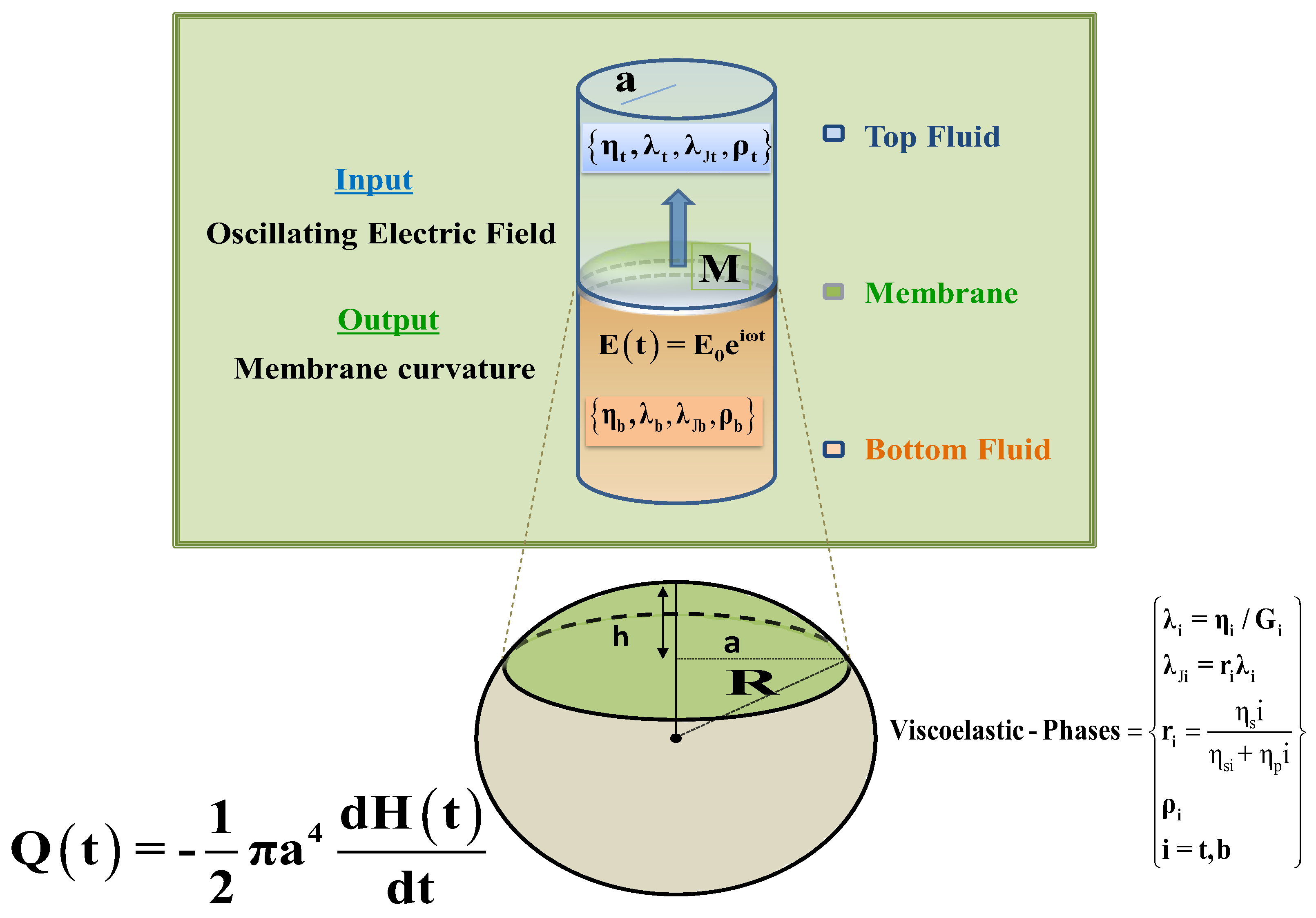
The physical setup and geometry of the flexoelectric membrane tethered to a capillary tube containing two viscoelastic fluids is defined in Figure 2.

A capillary tube of radius “a” contains an edge-fixed flexoelectric membrane located at z = 0. Above and below the membrane there are two Jeffrey’s viscoelastic incompressible fluids with column heights z = L, solvent viscosities {η_sb, η_st}, polymer viscosities {η_pb, η_pt}, relaxation times {λ_b, λ_t}, and densities {ρ_b, ρ_t}. The total viscosity, relaxation and Jeffreys times can be expressed:

$$\begin{array}{c}{\mathsf{\eta }}_{\mathrm{i}}=\left({\mathsf{\eta }}_{\mathrm{si}}+{\mathsf{\eta }}_{\mathrm{pi}}\right);{\mathsf{\lambda }}_{\mathrm{i}}={\mathsf{\eta }}_{\mathrm{i}}/{\mathrm{G}}_{\mathrm{i}}=\left({\mathsf{\eta }}_{\mathrm{si}}+{\mathsf{\eta }}_{\mathrm{pi}}\right)/{\mathrm{G}}_{\mathrm{i}};{\mathsf{\lambda }}_{\mathrm{Ji}}=\left({\mathsf{\eta }}_{\mathrm{si}}/{\mathsf{\eta }}_{\mathrm{si}}+{\mathsf{\eta }}_{\mathrm{pi}}\right){\mathsf{\lambda }}_{\mathrm{i}}\\ \mathrm{i}=\left\{\mathrm{t},\mathrm{p}\right\};\mathrm{t}:\mathrm{top},\mathrm{b}:\mathrm{bottom}\end{array}$$

The pressures at the top of the upper layer and at the bottom of the lower layers are equal to a constant p (z = 0) = p (z = L) = p₀. By imposing a fluctuating electrical field E(t) in the bottom, the membrane oscillates and displaces the upper and lower incompressible viscoelastic fluids; we emphasize that the Poiseuille flow is only generated by the flexoelectric effect of the membrane caused by the imposed E(t) field, and body forces are neglected (null gravitational mechanisms) [9,10,12].

The membranodynamic system contains the following primitive materials properties: (i) fluids viscoelastic properties $\{{\mathsf{\eta }}_{\mathrm{b}}{,\mathsf{\lambda }}_{\mathrm{b}}{,\mathsf{\lambda }}_{\mathrm{Jb}},{\mathsf{\eta }}_{\mathrm{t}}{,\mathsf{\lambda }}_{\mathrm{t}},{\mathsf{\lambda }}_{\mathrm{Jt}}\}$; (ii) membrane elasticity properties:$\{{\mathsf{\gamma }}_{\mathrm{o}},{\mathrm{k}}_{\mathrm{c}}{,\overline{\mathrm{k}}}_{\mathrm{c}}\}$; (iii) geometry of the pipe and the membrane $\left\{\mathrm{a},\mathrm{L};\mathsf{\Im }\right\}$; and (iv) flexoelectric force: {c_f, E₀}. The elastic moduli of the viscoelastic fluids are: G_i =η_i/λ_i; i = t, b. These parameters can be estimated from rheological and membrane experiments in steady and unsteady state [9,10] (and references therein).

2.1. Dimensionless Governing Equations

The coupled governing device equations are the dimensionless shape model, which is a force balance between the electrical field, pressure balance, and elastic storage membrane [9,10,12]. The second equationis is the pressure balance with emerges of the momentum equation (Equation (2a)) and the total temporal viscosity operator, which is the sum of the top and bottom liquid viscoelastic phases [12], which can be extended by any linear and non-linear viscoelastic equation [9,12]. In order to simplify the problem, dimensionless variables are used in the main equations to obtain dimensionless groups that facilitate the physical interpretation (see Appendix A). The dimensionless shape equation is given by:

$${\mathrm{a}}_0^{*}\overline{\mathrm{E}}\left(\overline{\mathrm{t}}\right)=\frac{1}{4}\frac{\overline{\Delta \mathrm{p}}\left(\overline{\mathrm{t}}\right)}{\mathrm{L}}+\overline{\mathrm{M}}\overline{\mathrm{H}}\left(\overline{\mathrm{t}}\right)=\frac{1}{4}\frac{\overline{\Delta \mathrm{p}}\left(\overline{\mathrm{t}}\right)}{\mathrm{L}}+\frac{1-\mathrm{k}}{\mathrm{k}}\overline{\mathrm{H}}\left(\overline{\mathrm{t}}\right);$$

(1a)

$$\overline{\mathrm{M}}=\frac{1-\mathrm{k}}{\mathrm{k}}$$

(1b)

The pressure balance and the time viscosity operator are given by:

$$\overline{\frac{\Delta \mathrm{p}}{\mathrm{L}}}\left(\overline{\mathrm{t}}\right)=\left\{\left(\overline{\mathsf{\eta }}\left({\mathrm{D}}_{\overline{\mathrm{t}}}\right)\right)\frac{1}{\overline{\mathrm{r}}}\frac{\partial }{\partial \overline{\mathrm{r}}}\overline{\mathrm{r}}\frac{\partial }{\partial \overline{\mathrm{r}}}-{\mathrm{Ma}}^2{\mathrm{D}}_{\overline{\mathrm{t}}}\right\}\overline{\mathrm{V}}\mathrm{z}\left(\overline{\mathrm{r}},\overline{\mathrm{t}}\right);$$

(2a)

$$\overline{\mathsf{\eta }}\left({\mathrm{D}}_{\overline{\mathrm{t}}}\right)={\overline{\mathsf{\eta }}}_{\mathrm{t}}\left({\mathrm{D}}_{\overline{\mathrm{t}}}\right)+{\overline{\mathsf{\eta }}}_{\mathrm{b}}\left({\mathrm{D}}_{\overline{\mathrm{t}}}\right)$$

(2b)

In Equation (2), the Mach $\mathrm{Ma}$ and flexoelectric ${\mathrm{a}}_0^{*}$ numbers are given by:

$$\mathrm{Ma}=\frac{\mathrm{a}/\left({\mathsf{\lambda }}_{\mathrm{t}}{+\mathsf{\lambda }}_{\mathrm{b}}\right)}{\sqrt{\left({\mathrm{G}}_{\mathrm{t}}{+\mathrm{G}}_{\mathrm{b}}\right)/\left({\mathsf{\rho }}_{\mathrm{t}}+{\mathsf{\rho }}_{\mathrm{b}}\right)}};$$

(3a)

$${\mathrm{a}}_0^{*}=\frac{{\mathrm{c}}_{\mathrm{f}}\mathsf{\Im }{\mathrm{E}}_0\mathrm{a}/4\mathrm{L}}{{\mathrm{G}}_{\mathrm{t}}{+\mathrm{G}}_{\mathrm{b}}}$$

(3b)

The parameters and scaling details of Equations (1)–(3) are given in Appendix A. Equation (2a) is the z component of the momentum equation, which is a balance between the pressure gradient, and viscous and inertia mechanisms. The total viscosity operator given in Equation (2b) is completely general and can be used with any viscoelastic and fracctional viscoelastic model (See

Table 1. Different time viscoelastic operator.

Constitutive Equation	Mach Number	Lineal Viscosity Operator	Mathematical Approach	Ref.
Maxwell fluid without inertia	$\mathrm{M}\mathrm{a}=0$	$\overline{\mathsf{\eta }}\left({\mathrm{D}}_{\overline{\mathrm{t}}}\right)=\frac{{\overline{\mathsf{\eta }}}_{\mathrm{t}}}{1+{\overline{\mathsf{\lambda }}}_{\mathrm{t}}{\mathrm{D}}_{\overline{\mathrm{t}}}}+\frac{{\overline{\mathsf{\eta }}}_{\mathrm{b}}}{1+{\overline{\mathsf{\lambda }}}_{\mathrm{b}}{\mathrm{D}}_{\overline{\mathrm{t}}}}$	Second order differential Equation	[10,12]
Jeffreys fluid without inertia	$\mathrm{M}\mathrm{a}=0$	$\overline{\mathsf{\eta }}\left({\mathrm{D}}_{\overline{\mathrm{t}}}\right)={\overline{\mathsf{\eta }}}_{\mathrm{t}}\frac{1+{\overline{\mathsf{\lambda }}}_{\mathrm{J}\mathrm{t}}{\mathrm{D}}_{\overline{\mathrm{t}}}}{1+{\overline{\mathsf{\lambda }}}_{\mathrm{t}}{\mathrm{D}}_{\overline{\mathrm{t}}}}+{\overline{\mathsf{\eta }}}_{\mathrm{b}}\frac{1+{\overline{\mathsf{\lambda }}}_{\mathrm{J}\mathrm{b}}{\mathrm{D}}_{\overline{\mathrm{t}}}}{1+{\overline{\mathsf{\lambda }}}_{\mathrm{b}}{\mathrm{D}}_{\overline{\mathrm{t}}}}$	Third order differential Equation	Present Model

). Notice that ${\mathrm{D}}_{\overline{\mathrm{t}}}$ is a time differential operator which is defined by ${\mathrm{D}}_{\overline{\mathrm{t}}}=\partial /{\partial }_{\overline{\mathrm{t}}}$. In particular, in this research the Jeffreys viscosity model will be used, in order to obtain a third-order ODE that will describe the physics in this system. Combining Equations (1)–(3), the dynamical expression in terms of the Mach number is given by:

$$\left\{\left(\frac{1}{\overline{\mathrm{r}}}\frac{\partial }{\partial \overline{\mathrm{r}}}\overline{\mathrm{r}}\right)\frac{\partial }{\partial \overline{\mathrm{r}}}+{\overline{\mathsf{\beta }}}^2\right\}\overline{\mathrm{V}}\mathrm{z}\left(\overline{\mathrm{r}},\overline{\mathrm{t}}\right)=\frac{{\mathrm{a}}_0^{\ast }\overline{\mathrm{E}}\left(\overline{\mathrm{t}}\right)-\left({\mathrm{k}}^{-1}-1\right)\overline{\mathrm{H}}\left(\overline{\mathrm{t}}\right)}{\overline{\mathsf{\eta }}\left({\mathrm{D}}_{\overline{\mathrm{t}}}\right)};$$

(4a)

$${\overline{\mathsf{\beta }}}^2=-\frac{{\mathrm{Ma}}^2}{\overline{\mathsf{\eta }}\left({\mathrm{D}}_{\overline{\mathrm{t}}}\right)}{\mathrm{D}}_{\overline{\mathrm{t}}}$$

(4b)

where the parameter $\overline{\mathsf{\beta }}$ is the inverse of a characteristic length associated to the Mach number divided by the viscosity and multiplied by the time differential operator related to the inertia mechanisms. The solution of Equation (4) was already obtained in [12] for a Maxwell fluid (see Appendix B of reference [12]). Assuming non-slip conditions, i.e., $\overline{\mathrm{V}}\mathrm{z}\left(\overline{\mathrm{r}}=1,\overline{\mathrm{t}}\right)=0$ and that the system must be bounded at $\overline{\mathrm{r}}=0$, the dimensionless non-homogeneous parametric Bessel differential equation is obtained. Once the velocity profile is obtained, the volumetric flow can be easily obtained using the Bessel function properties (see Appendix B of reference [12]). The dimensionless volumetric flow $\overline{\mathrm{Q}}$ induced by the oscillations of the membrane in the viscoelastic phases, can be calculated from an integration in cylindrical coordinates:

$$\overline{\mathrm{Q}}\left(\overline{\mathrm{t}}\right)={\displaystyle \underset{0}{\overset{1}{\int }}\overline{\mathrm{V}}\mathrm{z}\left(\overline{\mathrm{r}},\overline{\mathrm{t}}\right)}\overline{\mathrm{r}}\mathrm{d}\overline{\mathrm{r}}=-\frac{{\mathrm{a}}_0^{*}\overline{\mathrm{E}}\left(\overline{\mathrm{t}}\right)-\left({\mathrm{k}}^{-1}-1\right)\overline{\mathrm{H}}\left(\overline{\mathrm{t}}\right)}{8\overline{\mathsf{\Pi }}\left({\mathrm{D}}_{\overline{\mathrm{t}}}\right)};$$

(5a)

$$\overline{\mathsf{\Pi }}\left({\mathrm{D}}_{\overline{\mathrm{t}}}\right)=\frac{\mathrm{M}{\mathrm{a}}^2{\mathrm{D}}_{\overline{\mathrm{t}}}/8}{1-2\frac{{\mathrm{J}}_1\left(\overline{\mathsf{\beta }}\right)/\overline{\mathsf{\beta }}}{{\mathrm{J}}_0\left(\overline{\mathsf{\beta }}\right)}}$$

(5b)

In Equation (5) the following property of the Bessel functions was used: xⁿ⁺¹J_n(x) = d[x J₁(x)]/dx = x J₀(x); and $\overline{\mathsf{\Pi }}\left({\mathrm{D}}_{\overline{\mathrm{t}}}\right)$ can be interpreted as inertia-viscous non-linear differential operator $\overline{\mathsf{\Pi }}\left({\mathrm{D}}_{\overline{\mathrm{t}}}\right)$, and the parameter $\overline{\mathsf{\beta }}$ was defined in Equation (4b). In the next step, the definition of the dimensionless volumetric flow is applied as the negative of the average membrane curvature time derivative [9,10,12], i.e.,:

$$\overline{\mathrm{Q}}\left(\overline{\mathrm{t}}\right)=-2^{-1}{\mathrm{D}}_{\overline{\mathrm{t}}}\overline{\mathrm{H}}\left(\overline{\mathrm{t}}\right)$$

(6)

Combining Equations (5) and (6) gives:

$${\overline{\mathrm{O}}}_{\mathsf{\alpha }}\left(\overline{\mathrm{t}}\right)=\left(\begin{array}{c}\overline{\mathrm{H}}\left(\overline{\mathrm{t}}\right):\mathsf{\alpha }=0\\ \overline{\mathrm{Q}}\left(\overline{\mathrm{t}}\right):\mathsf{\alpha }=1\end{array}\right)={\overline{\mathrm{R}}}_{\mathsf{\alpha }}\left({\mathrm{D}}_{\overline{\mathrm{t}}}\right)\overline{\mathrm{E}}\left(\overline{\mathrm{t}}\right);\mathsf{\alpha }=0,1$$

(7)

Equation (7) is the general non-linear dynamical expression and can be expressed in terms of an Input (electrical field E) and Output functions (average membrane curvature H or the volumetric flow rate Q). The corresponding transfer functions ${\overline{\mathrm{R}}}_1\left({\mathrm{D}}_{\overline{\mathrm{t}}}\right)$ and ${\overline{\mathrm{R}}}_2\left({\mathrm{D}}_{\overline{\mathrm{t}}}\right)$ are given by:

$${\overline{\mathrm{R}}}_0\left({\mathrm{D}}_{\overline{\mathrm{t}}}\right)=\frac{{\mathrm{a}}_0^{*}}{\overline{\mathsf{\Pi }}\left({\mathrm{D}}_{\overline{\mathrm{t}}}\right){\mathrm{D}}_{\overline{\mathrm{t}}}+{\mathrm{k}}^{-1}-1};$$

(8a)

$${\overline{\mathrm{R}}}_1\left({\mathrm{D}}_{\overline{\mathrm{t}}}\right)=-\frac{1}{2}\frac{{\mathrm{a}}_0^{*}}{\overline{\mathsf{\Pi }}\left({\mathrm{D}}_{\overline{\mathrm{t}}}\right)+\left({\mathrm{k}}^{-1}-1\right){\displaystyle \underset{0}{\overset{\mathsf{\alpha }}{\int }}\mathrm{d}\overline{\mathrm{t}}}}$$

(8b)

Equations (7) and (8) are non-linear differential equations that describe the relationship between the volumetric flow rate or the average membrane curvature and the electrical field E. In Equation (8b) it was assumed that the average membrane curvature is zero at time $\overline{\mathrm{t}}=0$. On the other hand, Equation (8a) represents the dynamic evolution of the input (electrical field) and the output (average membrane curvature), and Equation (8b) is the transfer function of the (electrical field) and the output (volumetric flow rate), respectively. Notice both of them are regulated by the flexoelectric mechanisms through the dimensionless number ${\mathrm{a}}_0^{*}$ asociated to the flexoelectric and viscoelastic mechanism through the time viscosity operator. Finally, both Equations (7) and (8) are the main model formulation results of this work.

2.2. Jeffrey’s Third-Order Ordinary Differential Equations

If the Bessel functions of the viscous-inertia defined in the operator $\overline{\mathsf{\Pi }}\left({\mathrm{D}}_{\overline{\mathrm{t}}}\right)$ of Equation (8) are developed in a Mach (Ma << 1), number power series (see Appendix B of [12]), the inertia-viscous operator $\overline{\mathsf{\Pi }}\left({\mathrm{D}}_{\overline{\mathrm{t}}}\right)$ is the sum of the total viscosity, i.e., $\overline{\mathsf{\Pi }}\left({\mathrm{D}}_{\overline{\mathrm{t}}}\right)\cong \overline{\mathsf{\eta }}\left({\mathrm{D}}_{\overline{\mathrm{t}}}\right)={\overline{\mathsf{\eta }}}_{\mathrm{t}}\left({\mathrm{D}}_{\overline{\mathrm{t}}}\right)+{\overline{\mathsf{\eta }}}_{\mathrm{b}}\left({\mathrm{D}}_{\overline{\mathrm{t}}}\right)$. In order to characterize the rheology and flow, the Jeffrey’s viscosity operator was used (Table 1), which is the minimum model to obtain the non-monotonically behavior in the power spectrum, and is given by:

$$\overline{\mathsf{\eta }}\left({\mathrm{D}}_{\overline{\mathrm{t}}}\right)={\overline{\mathsf{\eta }}}_{\mathrm{t}}\left({\mathrm{D}}_{\overline{\mathrm{t}}}\right)+{\overline{\mathsf{\eta }}}_{\mathrm{b}}\left({\mathrm{D}}_{\overline{\mathrm{t}}}\right)=\frac{{\mathsf{\Sigma }}_{\overline{\mathsf{\eta }}}+\left({\overline{\mathsf{\lambda }}}_{\mathrm{t}}{\overline{\mathsf{\lambda }}}_{\mathrm{b}}+{\mathsf{\Sigma }}_{\overline{\mathsf{\lambda }}{\overline{\mathsf{\eta }}}_{\mathrm{J}}}\right){\mathrm{D}}_{\overline{\mathrm{t}}}+{\mathsf{\Sigma }}_{{\overline{\mathsf{\eta }}}_{\mathrm{J}}}{\overline{\mathsf{\lambda }}}_{\mathrm{t}}{\overline{\mathsf{\lambda }}}_{\mathrm{b}}{\mathrm{D}}_{{\overline{\mathrm{t}}}^2}^2}{1+{\mathrm{D}}_{\overline{\mathrm{t}}}+{\overline{\mathsf{\lambda }}}_{\mathrm{t}}{\overline{\mathsf{\lambda }}}_{\mathrm{b}}{\mathrm{D}}_{{\overline{\mathrm{t}}}^2}^2}$$

(9)

Once Equation (9) is substituted into Equations (8), and using the linear relation Equation (7), the following third-order differential equation in terms of an input variable {E(t)} and output variables {H(t), Q(t)} is obtained:

$${\mathrm{L}}_{{\overline{\mathrm{O}}}_{\mathsf{\alpha }}}^3\left\{{\overline{\mathrm{O}}}_{\mathsf{\alpha }}\left(\overline{\mathrm{t}}\right)\right\}={\mathrm{a}}_0^{*}\frac{1-\mathrm{k}}{\mathrm{k}}{\left(-\frac{1}{2}\right)}^{\mathsf{\alpha }}{\mathrm{L}}_{{\overline{\mathrm{I}}}_{\mathsf{\alpha }}}^3\left\{\overline{\mathrm{E}}\left(\overline{\mathrm{t}}\right)\right\};$$

(10a)

$${\overline{\mathrm{O}}}_{\mathsf{\alpha }}\left(\overline{\mathrm{t}}\right)=\left(\begin{array}{c}\overline{\mathrm{H}}\left(\overline{\mathrm{t}}\right):\mathsf{\alpha }=0\\ \overline{\mathrm{Q}}\left(\overline{\mathrm{t}}\right):\mathsf{\alpha }=1\end{array}\right)$$

(10b)

The output and input linear operators are given by the following differential operators:

$${\mathrm{L}}_{{\overline{\mathrm{O}}}_{\mathsf{\alpha }}}^3=\underset{\mathrm{Retardation}}{\underbrace{{\mathrm{b}}_3^{*}{\mathrm{D}}_{\overline{\mathrm{t}}}^3}}+\underset{\mathrm{Inertia}}{\underbrace{{\mathrm{b}}_2^{*}{\mathrm{D}}_{\overline{\mathrm{t}}}^2}}+\underset{\mathrm{Viscous}-\mathrm{Bulk}}{\underbrace{{\mathrm{b}}_1^{*}{\mathrm{D}}_{\overline{\mathrm{t}}}^1}}+\underset{\mathrm{Elastic}-\mathrm{Membrane}}{\underbrace{{\mathrm{b}}_0^{*}}};$$

(11a)

$${\mathrm{L}}_{{\overline{\mathrm{I}}}_{\mathsf{\alpha }}}^3=\underset{\mathrm{Inertia}}{\underbrace{{\mathrm{a}}_2^{*}{\mathrm{D}}_{{\overline{\mathrm{t}}}^{2+\mathsf{\alpha }}}^{2+\mathsf{\alpha }}}}+\underset{\mathrm{Viscous}-\mathrm{Bulk}}{\underbrace{{\mathrm{a}}_1^{*}{\mathrm{D}}_{{\overline{\mathrm{t}}}^{1+\mathsf{\alpha }}}^{1+\mathsf{\alpha }}}}+\underset{\mathrm{Elastic}-\mathrm{Membrane}}{\underbrace{{\mathrm{D}}_{{\overline{\mathrm{t}}}^{\mathsf{\alpha }}}^{\mathsf{\alpha }}}}$$

(11b)

The dimensionless coefficients of Equations (9)–(11) are given by:

$$\mathrm{Jeffrey}\prime \mathrm{s}\mathrm{Model}:\{\begin{array}{c}{\mathrm{a}}_0^{*}=\frac{{\mathrm{c}}_{\mathrm{f}}\mathsf{\Im }/4\mathrm{L}}{\mathrm{Gt}+\mathrm{Gb}},{\mathrm{a}}_1^{*}=1,{\mathrm{a}}_2^{*}={\overline{\mathsf{\lambda }}}_{\mathrm{t}}{\overline{\mathsf{\lambda }}}_{\mathrm{b}}\hfill \\ {\mathrm{b}}_0^{*}=1,{\mathrm{b}}_1^{*}=1+\left(\frac{1-\mathrm{k}}{\mathrm{k}}\right){\mathsf{\Sigma }}_{\overline{\mathsf{\eta }}},{\mathrm{b}}_2^{*}=\frac{{\overline{\mathsf{\lambda }}}_{\mathrm{t}}{\overline{\mathsf{\lambda }}}_{\mathrm{b}}}{\mathrm{k}}+\frac{1-\mathrm{k}}{\mathrm{k}}{\mathsf{\Sigma }}_{\overline{\mathsf{\lambda }}{\overline{\mathsf{\eta }}}_{\mathrm{J}}},{\mathrm{b}}_3^{*}=\frac{1-\mathrm{k}}{\mathrm{k}}{\overline{\mathsf{\lambda }}}_{\mathrm{t}}{\overline{\mathsf{\lambda }}}_{\mathrm{b}}{\mathsf{\Sigma }}_{{\overline{\mathsf{\eta }}}_{\mathrm{J}}}\hfill \\ {\mathsf{\Sigma }}_{{\overline{\mathsf{\eta }}}_{\mathrm{J}}}={\overline{\mathsf{\eta }}}_{\mathrm{Jt}}+{\overline{\mathsf{\eta }}}_{\mathrm{Jb}}={\overline{\mathrm{G}}}_{\mathrm{t}}{\overline{\mathsf{\lambda }}}_{\mathrm{Jt}}+{\overline{\mathrm{G}}}_{\mathrm{b}}{\overline{\mathsf{\lambda }}}_{\mathrm{Jb}}={\mathrm{r}}_{\mathrm{t}}{\overline{\mathrm{G}}}_{\mathrm{t}}{\overline{\mathsf{\lambda }}}_{\mathrm{t}}{+\mathrm{r}}_{\mathrm{b}}{\overline{\mathrm{G}}}_{\mathrm{b}}{\overline{\mathsf{\lambda }}}_{\mathrm{b}}={\mathrm{r}}_{\mathrm{t}}{\overline{\mathsf{\eta }}}_{\mathrm{t}}{+\mathrm{r}}_{\mathrm{b}}{\overline{\mathsf{\eta }}}_{\mathrm{b}}\hfill \\ {\mathsf{\Sigma }}_{\mathsf{\lambda }{\overline{\mathsf{\eta }}}_{\mathrm{J}}}={\overline{\mathsf{\lambda }}}_{\mathrm{t}}{\overline{\mathsf{\eta }}}_{\mathrm{Jt}}+{\overline{\mathsf{\lambda }}}_{\mathrm{b}}{\overline{\mathsf{\eta }}}_{\mathrm{Jb}}={\overline{\mathsf{\lambda }}}_{\mathrm{t}}{\overline{\mathrm{G}}}_{\mathrm{t}}{\overline{\mathsf{\lambda }}}_{\mathrm{Jt}}+{\overline{\mathsf{\lambda }}}_{\mathrm{b}}{\overline{\mathrm{G}}}_{\mathrm{b}}{\overline{\mathsf{\lambda }}}_{\mathrm{Jb}}={\mathrm{r}}_{\mathrm{t}}{\overline{\mathsf{\lambda }}}_{\mathrm{t}}{\overline{\mathsf{\eta }}}_{\mathrm{t}}{+\mathrm{r}}_{\mathrm{b}}{\overline{\mathsf{\lambda }}}_{\mathrm{b}}{\overline{\mathsf{\eta }}}_{\mathrm{b}}\hfill \\ {\mathrm{r}}_{\mathrm{i}}={\mathsf{\eta }}_{\mathrm{s}}{}_{\mathrm{i}}/\left({\mathsf{\eta }}_{\mathrm{s}}{}_{\mathrm{i}}+{\mathsf{\eta }}_{\mathrm{p}}{}_{\mathrm{i}}\right);\mathrm{i}=\left\{\mathrm{t},\mathrm{p}\right\}\hfill \end{array}$$

(12)

The first term on the left hand side of Equation (11a) describes the retardation forces, the second and third terms are associated with inertia and viscous mechanisms, respectively; and the last one with the membrano-elastic mechanisms. The right-hand side describes the temporal evolution of the input driven force associated with flexo-electric mechanisms and the memory through the material parameters of the particular constitutive equation used in the system. A Newtonian model was obtained in [9], a Maxwell second-order electro-rheological model was previously obtained in [10,12] using different mathematical approaches, and this Maxwell model was extended by taking into account the inertial mechanisms of the momentum fluids and finally non-linear extension (Newtonian) of these models was studied with a pertubation technique in terms of the Deborah number [9,10,12].

2.2.1. Dimensionless Numbers

The governing Equations (11) and (12) contain seven dimensionless numbers:

$$\left\{{\mathrm{a}}_0^{*},{\overline{\mathsf{\lambda }}}_{\mathrm{t}}{\overline{\mathsf{\lambda }}}_{\mathrm{b}},\mathrm{k},\mathrm{Ma},{\mathsf{\Sigma }}_{\overline{\mathsf{\eta }}}{,\mathsf{\Sigma }}_{{\overline{\mathsf{\eta }}}_{\mathrm{J}}}{,\mathsf{\Sigma }}_{\overline{\mathsf{\lambda }}{\overline{\mathsf{\eta }}}_{\mathrm{J}}}\right\}$$

(13)

which are associated with the following mechanisms: (i) Memory $\left({\overline{\mathsf{\lambda }}}_{\mathrm{t}}{\overline{\mathsf{\lambda }}}_{\mathrm{b}}\right)$: product of the viscoelastic dimensionless times ${\overline{\mathsf{\lambda }}}_{\mathrm{t}}$, and ${\overline{\mathsf{\lambda }}}_{\mathrm{b}}$, where ${\overline{\mathsf{\lambda }}}_{\mathrm{t}}+{\overline{\mathsf{\lambda }}}_{\mathrm{b}}=1$. This number ${\overline{\mathsf{\lambda }}}_{\mathrm{t}}{\overline{\mathsf{\lambda }}}_{\mathrm{b}}$ defines the elastic asymmetry of the fluids. When ${\overline{\mathsf{\lambda }}}_{\mathrm{t}}{\overline{\mathsf{\lambda }}}_{\mathrm{b}}<<1$ (highly asymmetric case) one of the fluids is nearly inelastic, and when ${\overline{\mathsf{\lambda }}}_{\mathrm{t}}{\overline{\mathsf{\lambda }}}_{\mathrm{b}}=1/4$ (highly symmetric case) both fluids are equally elastic; (ii) Bulk Viscosity $\left({\mathsf{\Sigma }}_{\overline{\mathsf{\eta }}}={\overline{\mathsf{\eta }}}_{\mathrm{t}}+{\overline{\mathsf{\eta }}}_{\mathrm{b}}={\overline{\mathrm{G}}}_{\mathrm{t}}{\overline{\mathsf{\lambda }}}_{\mathrm{t}}+{\overline{\mathrm{G}}}_{\mathrm{b}}{\overline{\mathsf{\lambda }}}_{\mathrm{b}}\right)$: total viscosity in the system, where the elastic dimensionless moduli satisfy ${\overline{\mathrm{G}}}_{\mathrm{t}}+{\overline{\mathrm{G}}}_{\mathrm{b}}=1$. The numerical value of this number is controlled by the product between the two dimensionless Maxwell time numbers, i.e., ${\mathsf{\Sigma }}_{\overline{\mathsf{\eta }}}{=\mathsf{\Sigma }}_{\overline{\mathsf{\eta }}}\left({\overline{\mathsf{\lambda }}}_{\mathrm{t}}{\overline{\mathsf{\lambda }}}_{\mathrm{b}}\right)$. This dimensionless number is bounded by the maximum and minimum values of the Maxwell relaxation times, i.e., $\left\{{\overline{\mathsf{\lambda }}}_{\mathrm{t}},{\overline{\mathsf{\lambda }}}_{\mathrm{b}}\right\}{=\mathsf{\Sigma }}_{\overline{\mathsf{\eta }}\min }\le {\mathsf{\Sigma }}_{\overline{\mathsf{\eta }}}{=\mathsf{\Sigma }}_{\overline{\mathsf{\eta }}}\left({\overline{\mathsf{\lambda }}}_{\mathrm{t}}{\overline{\mathsf{\lambda }}}_{\mathrm{b}}\right)\le {\mathsf{\Sigma }}_{\overline{\mathsf{\eta }}\max }=\left\{{\overline{\mathsf{\lambda }}}_{\mathrm{t}},{\overline{\mathsf{\lambda }}}_{\mathrm{b}}\right\}$; (iii) The third group, ${\mathsf{\Sigma }}_{{\overline{\mathsf{\eta }}}_{\mathrm{J}}}={\overline{\mathsf{\eta }}}_{\mathrm{Jt}}+{\overline{\mathsf{\eta }}}_{\mathrm{Jb}}$ can be interpreted as a bulk viscosity weighted by the ratio between the solvent and total viscosity (solvent + polymer contributions). This dimensionless number is bounded by the following inequality: $\left\{{\mathrm{r}}_{\mathrm{t}}{\overline{\mathsf{\lambda }}}_{\mathrm{t}},{\mathrm{r}}_{\mathrm{b}}{\overline{\mathsf{\lambda }}}_{\mathrm{b}}\right\}{=\mathsf{\Sigma }}_{\overline{\mathsf{\eta }}\min }\le {\mathsf{\Sigma }}_{{\overline{\mathsf{\eta }}}_{\mathrm{J}}}{=\mathsf{\Sigma }}_{{\overline{\mathsf{\eta }}}_{\mathrm{J}}}\left({\overline{\mathsf{\lambda }}}_{\mathrm{t}}{\overline{\mathsf{\lambda }}}_{\mathrm{b}}\right)\le {\mathsf{\Sigma }}_{\overline{\mathsf{\eta }}\max }=\left\{{\mathrm{r}}_{\mathrm{t}}{\overline{\mathsf{\lambda }}}_{\mathrm{t}},{\mathrm{r}}_{\mathrm{b}}{\overline{\mathsf{\lambda }}}_{\mathrm{b}}\right\}$; (iv) The fourth group is a bulk retardation viscosity weighted by the viscoelastic relaxation times, i.e., ${\mathsf{\Sigma }}_{\mathsf{\lambda }{\overline{\mathsf{\eta }}}_{\mathrm{J}}}={\overline{\mathsf{\lambda }}}_{\mathrm{t}}{\overline{\mathsf{\eta }}}_{\mathrm{Jt}}+{\overline{\mathsf{\lambda }}}_{\mathrm{b}}{\overline{\mathsf{\eta }}}_{\mathrm{Jb}}$ can be interpreted as a bulk viscosity weighted by the product between the solvent ratio ${\mathrm{r}}_{\mathrm{i}}={\mathsf{\eta }}_{\mathrm{s}}{}_{\mathrm{i}}/\left({\mathsf{\eta }}_{\mathrm{s}}{}_{\mathrm{i}}+{\mathsf{\eta }}_{\mathrm{p}}{}_{\mathrm{i}}\right);\mathrm{i}=\left\{\mathrm{t},\mathrm{p}\right\}$ and the Maxwell relaxation times $\left({\overline{\mathsf{\lambda }}}_{\mathrm{t}},{\overline{\mathsf{\lambda }}}_{\mathrm{b}}=1-{\overline{\mathsf{\lambda }}}_{\mathrm{t}}\right)$. The maxima and minima values of this group are given by:

$$\left\{{\mathrm{r}}_{\mathrm{t}}{\overline{\mathsf{\lambda }}}_{\mathrm{t}}^2,{\mathrm{r}}_{\mathrm{b}}{\overline{\mathsf{\lambda }}}_{\mathrm{b}}^2\right\}{=\mathsf{\Sigma }}_{\overline{\mathsf{\lambda }}{\overline{\mathsf{\eta }}}_{\mathrm{J}}\min }\le {\mathsf{\Sigma }}_{\overline{\mathsf{\lambda }}{\overline{\mathsf{\eta }}}_{\mathrm{J}}}{=\mathsf{\Sigma }}_{\overline{\mathsf{\lambda }}{\overline{\mathsf{\eta }}}_{\mathrm{J}}}\left({\overline{\mathsf{\lambda }}}_{\mathrm{t}}{\overline{\mathsf{\lambda }}}_{\mathrm{b}}\right)\le {\mathsf{\Sigma }}_{\overline{\mathsf{\lambda }}{\overline{\mathsf{\eta }}}_{\mathrm{J}}\max }=\left\{{\mathrm{r}}_{\mathrm{t}}{\overline{\mathsf{\lambda }}}_{\mathrm{t}}^2,{\mathrm{r}}_{\mathrm{b}}{\overline{\mathsf{\lambda }}}_{\mathrm{b}}^2\right\}$$

(v) Elastic ratio $\left(\mathrm{k}\right)$: dimensionless ratio between the membrane and the total system elasticity, $0\text{<}={\left(1+1/\overline{\mathrm{M}}\right)}^{-1}<1$. A floppy (soft) and stiff (rigid) membrane corresponds to k << 1 and k ≅ 1, respectively. The elastic ratio, $\mathrm{k}=\mathrm{k}\left(\overline{\mathrm{M}}\right)$ is determined by the dimensionless elastic membrane modulus; (IV–V); (vi) The Mach number Ma is a ratio between the two velocities associated to viscoelasticity and bulk elastic forces and it is a measure of the inertia mechanism in the system; and finally (vii) the flexoelectric number ${\mathrm{a}}_0^{*}$ is the dimensionless conversion of electric to bulk elastic energy or, equivalently, the static transfer function at zero frequency.

2.2.2. Response Mode Classification

It was demonstrated for a Maxwell fluid [10,12], that the important resonant characteristics are dominated by four dimensionless numbers $\left\{{\overline{\mathsf{\lambda }}}_{\mathrm{t}}{\overline{\mathsf{\lambda }}}_{\mathrm{b}},{\mathsf{\Sigma }}_{\overline{\mathsf{\eta }}},\mathrm{k},{\mathrm{a}}_0^{*};{\mathrm{a}}_0^{*}=\mathrm{k}\right\}$. In the extended Jeffrey’s model (Equations (11)–(13)) additional numbers are obtained by including inertial and solvent mechanisms $\left\{\mathrm{Ma},{\mathsf{\Sigma }}_{{\overline{\mathsf{\eta }}}_{\mathrm{J}}}{,\mathsf{\Sigma }}_{\overline{\mathsf{\lambda }}{\overline{\mathsf{\eta }}}_{\mathrm{J}}}\right\}$ which can be interpreted as small perturbations to the previous Maxwell model [10,12]. According to the magnitudes of the main dimensionless numbers $\left\{{\overline{\mathsf{\lambda }}}_{\mathrm{t}}{\overline{\mathsf{\lambda }}}_{\mathrm{b}},{\mathsf{\Sigma }}_{\overline{\mathsf{\eta }}}{,\mathrm{k},\mathrm{a}}_0^{*}\right\}$, six case scenarios are possible i.e., the memory symmetry can be high (HS) or low (LS), the total viscosity high (HV), medium (MV), or low (LV), and the membrane can be floppy (FM) or stiff (SM), and these are summarized in

Table 2. Response modes I and III of the flexoelectric-viscoelastic device.

Material Conditions	Maxwell			Jeffrey’s
System’s Modes	${\overline{\mathsf{\lambda }}}_{\mathbf{t}}{\overline{\mathsf{\lambda }}}_{\mathbf{b}}$	${\mathsf{\Sigma }}_{\overline{\mathsf{\eta }}}={\mathsf{\Sigma }}_{\overline{\mathsf{\eta }}}\left({\overline{\mathsf{\lambda }}}_{\mathbf{t}}{\overline{\mathsf{\lambda }}}_{\mathbf{b}}\right)$	$\mathbf{k}=\mathsf{\epsilon }$	$\begin{array}{c}{\mathsf{\Sigma }}_{{\overline{\mathsf{\eta }}}_{\mathbf{J}}}={\mathsf{\Sigma }}_{{\overline{\mathsf{\eta }}}_{\mathbf{J}}}\left({\overline{\mathsf{\lambda }}}_{\mathbf{t}}{\overline{\mathsf{\lambda }}}_{\mathbf{b}}\right)\\ {\overline{\mathsf{\lambda }}}_{\mathrm{Ji}}={\mathrm{r}}_{\mathrm{i}}{\overline{\mathsf{\lambda }}}_{\mathrm{i}}\\ {\mathrm{r}}_{\mathrm{i}}={\mathsf{\eta }}_{\mathrm{si}}/{\mathsf{\eta }}_{\mathrm{si}}+{\mathsf{\eta }}_{\mathrm{pi}}\end{array}$	$\begin{array}{c}{\mathsf{\Sigma }}_{\overline{\mathsf{\lambda }}{\overline{\mathsf{\eta }}}_{\mathbf{J}}}={\mathsf{\Sigma }}_{\overline{\mathsf{\lambda }}{\overline{\mathsf{\eta }}}_{\mathbf{J}}}\left({\overline{\mathsf{\lambda }}}_{\mathbf{J}\mathbf{t}}{\overline{\mathsf{\lambda }}}_{\mathbf{J}\mathbf{b}}\right)\\ {\overline{\mathsf{\lambda }}}_{\mathrm{Ji}}={\mathrm{r}}_{\mathrm{i}}{\overline{\mathsf{\lambda }}}_{\mathrm{i}}\\ {\mathrm{r}}_{\mathrm{i}}={\mathsf{\eta }}_{\mathrm{si}}/{\mathsf{\eta }}_{\mathrm{si}}+{\mathsf{\eta }}_{\mathrm{pi}}\end{array}$
I {LS, LV, FM}	$\mathsf{\epsilon }$	$\mathsf{\epsilon }$	$\mathbf{k}=\mathsf{\epsilon }$	${\mathbf{r}}_{\mathbf{t}}\mathsf{\epsilon }<{\mathsf{\Sigma }}_{{\overline{\mathsf{\eta }}}_{\mathbf{J}}}<{\mathbf{r}}_{\mathbf{b}}$	${\mathbf{r}}_{\mathbf{t}}{\mathsf{\epsilon }}^2<{\mathsf{\Sigma }}_{\overline{\mathsf{\lambda }}{\overline{\mathsf{\eta }}}_{\mathbf{J}}}<{\mathbf{r}}_{\mathbf{b}}$
III {LS, HV, FM}	$\mathsf{\epsilon }$	$\mathbf{1}-\mathsf{\epsilon }$	$\mathbf{k}=\mathsf{\epsilon }$	${\mathbf{r}}_{\mathbf{t}}\mathsf{\epsilon }<{\mathsf{\Sigma }}_{{\overline{\mathsf{\eta }}}_{\mathbf{J}}}<{\mathbf{r}}_{\mathbf{b}}$	${\mathbf{r}}_{\mathbf{t}}{\mathsf{\epsilon }}^2<{\mathsf{\Sigma }}_{\overline{\mathsf{\lambda }}{\overline{\mathsf{\eta }}}_{\mathbf{J}}}<{\mathbf{r}}_{\mathbf{b}}$

The numerical value of ε = 10⁻⁴ and the polymer ratio r_i ∈ (0, 1): i = {t, b} and the value of $\mathbf{k}={\mathrm{a}}_0^{*}=\mathsf{\epsilon }$.

[10,12]. The third and fourth columns are the contributions of the Jeffrey’s retardation mechanisms $\left\{{\mathsf{\Sigma }}_{{\overline{\mathsf{\eta }}}_{\mathbf{J}}},{\mathsf{\Sigma }}_{\overline{\mathsf{\lambda }}{\overline{\mathsf{\eta }}}_{\mathbf{J}}}\right\}$, which are zero for the Maxwell model. For example, the first row {LS, LV, FM} corresponds to low symmetry, low viscosity, and floppy membrane [10,12]. This effective mode classification narrows the parametric envelope of biological significance. The specific numerical values in Table 2 are selected to be characteristic of each mode; the last two columns are bulk retardation and weighted retardation viscosity, respectively, which will be defined in the next section.

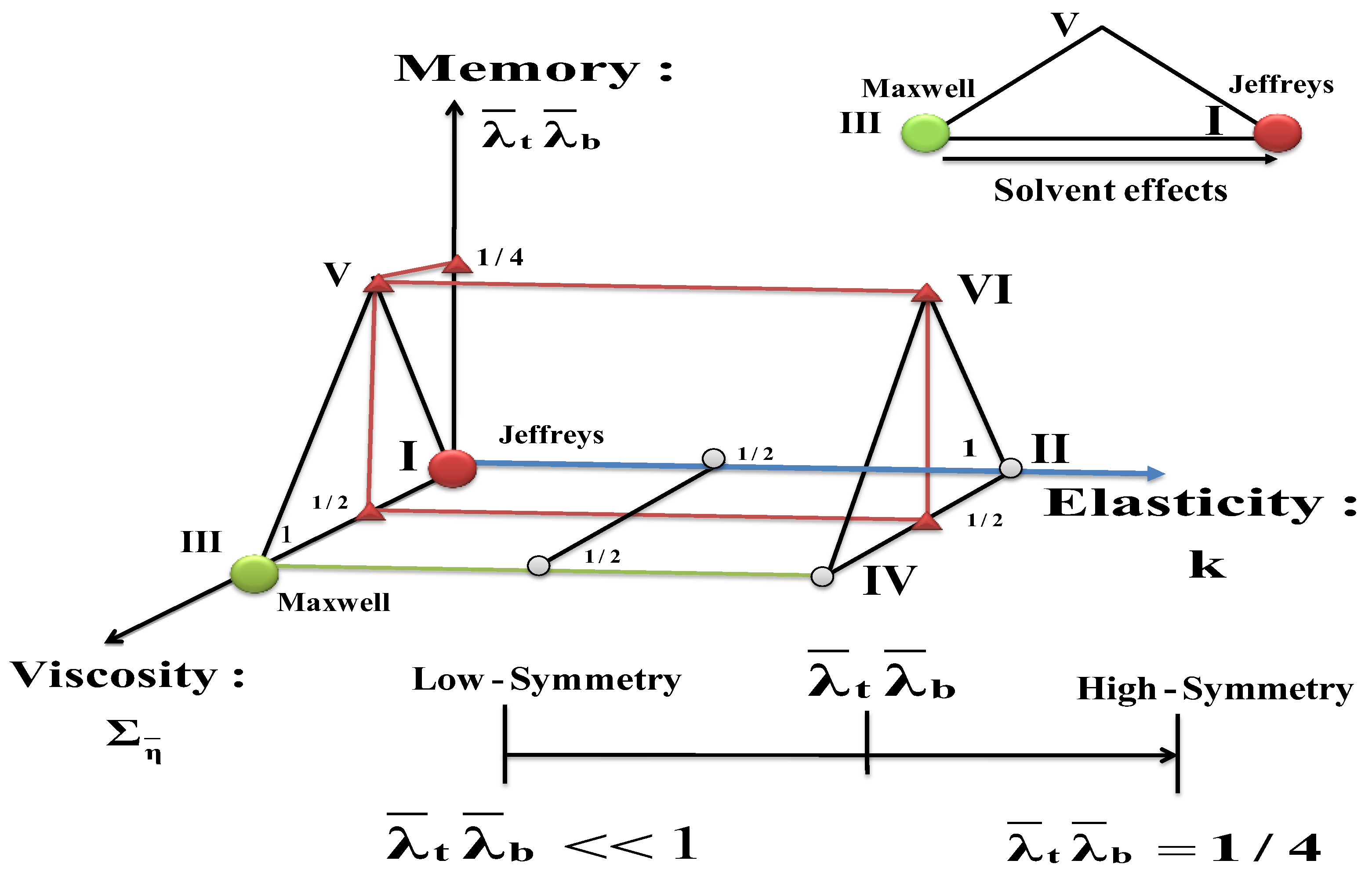
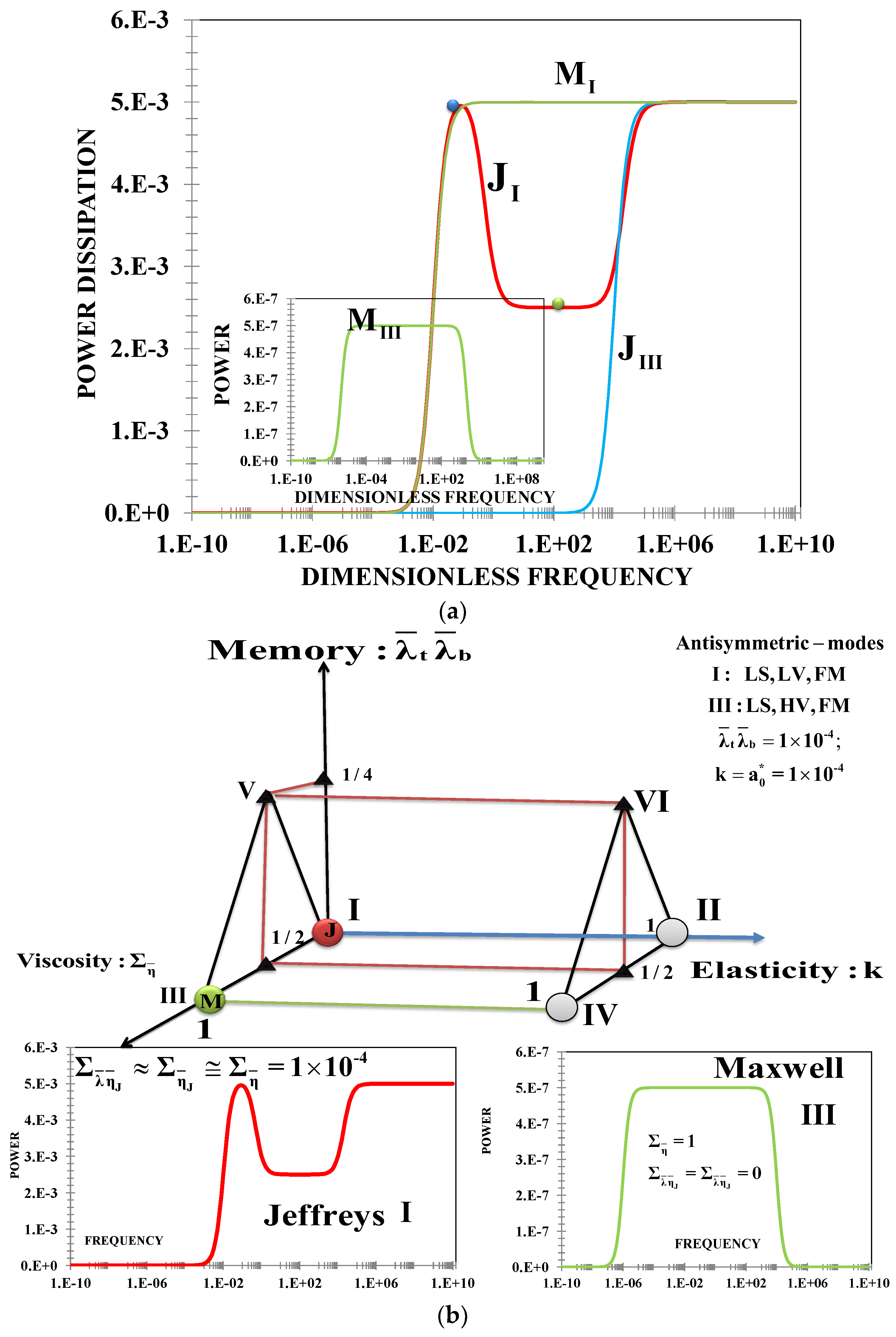
The six modes can be represented by the vertices of a prismatic 3D material space figure shown in Figure 3, spanned by fluid memory, membrane elasticity, and total fluid viscosity $\left\{{\overline{\mathsf{\lambda }}}_{\mathrm{t}}{\overline{\mathsf{\lambda }}}_{\mathrm{b}},{\mathsf{\Sigma }}_{\overline{\mathsf{\eta }}},\mathrm{k};\mathrm{k}={\mathrm{a}}_0^{*}\right\}$ respectively.

These dimensionless numbers are completely determined by the numerical value of the memory number ${\overline{\mathsf{\lambda }}}_{\mathrm{t}}{\overline{\mathsf{\lambda }}}_{\mathrm{b}}$ and solvent and viscosities ratio through r_i = 0. For example, in the case of the asymmetric case, given a small value of the memory number, i.e., ${\overline{\mathsf{\lambda }}}_{\mathrm{t}}{\overline{\mathsf{\lambda }}}_{\mathrm{b}}=\mathsf{\epsilon }<<1$, the respective minimum and maximum values of the Maxwell relaxation times are $\left({\overline{\mathsf{\lambda }}}_{\mathrm{t}}=\mathsf{\epsilon }<<1,{\overline{\mathsf{\lambda }}}_{\mathrm{b}}=1-\mathsf{\epsilon }\cong 1\right)$, the corresponding minimum and maximum values for the total bulk viscosity, bulk retardation viscosity, and weighted retardation viscosity are given by: ${\mathsf{\Sigma }}_{\overline{\mathsf{\eta }}}\in \left(\mathsf{\epsilon },1-\mathsf{\epsilon }\right)$; ${{\mathsf{\Sigma }}_{\overline{\mathsf{\eta }}}}_{\mathrm{J}}\in \left(\mathsf{\epsilon }{\mathrm{r}}_{\mathrm{t}},{\mathrm{r}}_{\mathrm{b}}\left(1-\mathsf{\epsilon }\right)\right)$ and the last one is ${\mathsf{\Sigma }}_{\overline{\mathsf{\lambda }}}{{}_{\overline{\mathsf{\eta }}}}_{{}_{\mathrm{J}}}\in \left({\mathsf{\epsilon }}^2{\mathrm{r}}_{\mathrm{t}},{\mathrm{r}}_{\mathrm{b}}\left(1-{\mathsf{\epsilon }}^2\right)\right)$. For the symmetric case, the value of the memory number is ${\overline{\mathsf{\lambda }}}_{\mathrm{t}}{\overline{\mathsf{\lambda }}}_{\mathrm{b}}=1/4$. Here, the Maxwell relaxation times are equal, i.e., ${\overline{\mathsf{\lambda }}}_{\mathrm{t}}={\overline{\mathsf{\lambda }}}_{\mathrm{b}}=1/2$, the bulk viscosity is fixed at ${\mathsf{\Sigma }}_{\overline{\mathsf{\eta }}}=1/2$ [10,12], and the values of the retardation bulk and average bulk viscosities can be chosen from the following ranges, ${\mathsf{\Sigma }}_{\overline{\mathsf{\eta }}}{}_{{}_{\mathrm{J}}}\in \left(\mathsf{\epsilon }{\mathrm{r}}_{\mathrm{t}},{\mathrm{r}}_{\mathrm{b}}\right)/2$ and ${\mathsf{\Sigma }}_{\overline{\mathsf{\lambda }}}{{}_{\overline{\mathsf{\eta }}}}_{{}_{\mathrm{J}}}\in \left(\mathsf{\epsilon }{\mathrm{r}}_{\mathrm{t}},{\mathrm{r}}_{\mathrm{b}}\right)/4$. The corresponding minimum and maximum values of the total bulk-viscosity (triangle) turn out to be a crucial material parameter in the energy conversion device. Finally, in this work we focus on the zone where the maximum and minimum of the Jeffrey’s model is found, and it is localized between modes I and III in the parametric 3D space, shown in Figure 3. The other modes, do not display resonance and antiresonance behavior [10,12].

3. Power Dissipation

The average power delivered to the viscoelastic fluids $\overline{\mathrm{P}}\left(\overline{\mathsf{\omega }}\right)$ by the oscillating membrane is the period average of the product of the input force $\mathrm{Re}\left[\overline{\mathrm{I}}\left(\overline{\mathrm{t}},\overline{\mathsf{\omega }}\right)\right]$ and the real part of the output $\mathrm{Re}\left[{\overline{\mathrm{O}}}_{\mathsf{\alpha }}\left(\overline{\mathrm{t}},\overline{\mathsf{\omega }}\right)\right]$ associated to the average membrane curvature or volumetric flow [9,10,12]:

$${\overline{\mathrm{P}}}_{\mathsf{\alpha }}\left(\overline{\mathsf{\omega }}\right)=\langle \mathrm{Re}\left[\overline{\mathrm{I}}\left(\overline{\mathrm{t}},\overline{\mathsf{\omega }}\right)\right]\cdot \mathrm{Re}\left[{\overline{\mathrm{O}}}_{\mathsf{\alpha }}\left(\overline{\mathrm{t}},\overline{\mathsf{\omega }}\right)\right]\rangle ;\mathsf{\alpha }=\{0,1\}$$

(14)

The power dissipation of the system can be calculated trough the transfer function of the average membrane curvature ${\mathrm{R}}_0\left(\overline{\mathsf{\omega }}\right)$, or in terms of volumetric transfer function, ${\mathrm{R}}_1\left(\overline{\mathsf{\omega }}\right)$:

$$\langle \overline{\mathrm{p}}\left(\overline{\mathsf{\omega }}\right)\rangle =\frac{1}{2}\left(\mathrm{Re}[{\overline{\mathrm{R}}}_1\left(\overline{\mathsf{\omega }}\right)]\right)=\frac{1}{2}\left|\overline{\mathsf{\omega }}\mathrm{Im}[{\overline{\mathrm{R}}}_0\left(\overline{\mathsf{\omega }}\right)]/2\right|$$

(15)

In order to compute Equation (15), the complex inertia-viscous function must be choosen from Table 1. Herrera-Valencia and Rey (2015) [12] use the Maxwell model and the properties of the power series up to the first sixth terms considereing the real and imaginary parts [12]. In this research, we consider all the terms of the dimesnionless parametric Bessel functions.

Inertialess Mechanisms: Ma << 1

In the case of small Mach number (Ma→0), the viscoelastic inertial mechanisms can be neglected and the power dissipation ${\overline{\mathrm{P}}}_{\mathsf{\alpha }}\left(\overline{\mathsf{\omega }}\right)$, α = 0, 1 is given by the following analytical expression:

$${\overline{\mathrm{P}}}_{\mathsf{\alpha }}\left(\overline{\mathsf{\omega }}\right)=\frac{1}{2}{\mathrm{a}}_0^{*}\frac{1-\mathrm{k}}{\mathrm{k}}\frac{\left({\mathrm{b}}_1^{*}-1\right){\overline{\mathsf{\omega }}}^2+\left(\left({1-\mathrm{kb}}_1^{*}\right){\mathrm{b}}_2^{*}+\left(1-\mathrm{k}\right){\mathsf{\Sigma }}_{\overline{\mathsf{\lambda }}{\overline{\mathsf{\eta }}}_{\mathrm{J}}}{\mathrm{b}}_1^{*}{-\mathrm{b}}_3^{*}\right){\overline{\mathsf{\omega }}}^4+\left({\mathrm{kb}}_2^{*}-\left(1-\mathrm{k}\right){\mathsf{\Sigma }}_{\overline{\mathsf{\lambda }}{\overline{\mathsf{\eta }}}_{\mathrm{J}}}\right){\mathrm{b}}_3^{*}{\overline{\mathsf{\omega }}}^6}{{\left({1-\mathrm{b}}_2^{*}{\overline{\mathsf{\omega }}}^2\right)}^2+{\overline{\mathsf{\omega }}}^2{\left({\mathrm{b}}_1^{*}{-\mathrm{b}}_3^{*}{\overline{\mathsf{\omega }}}^2\right)}^2}$$

(16)

The third terms of the numerator of Equation (16), can be rewritten in the following form:

$$\left({\mathrm{kb}}_2^{*}-\left(1-\mathrm{k}\right){\mathsf{\Sigma }}_{\overline{\mathsf{\lambda }}{\overline{\mathsf{\eta }}}_{\mathrm{J}}}\right){\mathrm{b}}_3^{*}={\mathrm{a}}_2^{*}{\mathrm{b}}_3^{*}={\left({\overline{\mathsf{\lambda }}}_{\mathrm{t}}{\overline{\mathsf{\lambda }}}_{\mathrm{b}}\right)}^2\left({\mathrm{k}}^{-1}-1\right){\mathsf{\Sigma }}_{{\overline{\mathsf{\eta }}}_{\mathrm{J}}}={\left({\overline{\mathsf{\lambda }}}_{\mathrm{t}}{\overline{\mathsf{\lambda }}}_{\mathrm{b}}\right)}^2\left({\mathrm{k}}^{-1}-1\right)\left({\mathrm{r}}_{\mathrm{t}}{\overline{\mathsf{\eta }}}_{\mathrm{t}}+{\mathrm{r}}_{\mathrm{b}}{\overline{\mathsf{\eta }}}_{\mathrm{b}}\right)$$

(17)

Equation (17) can be expressed in the following form:

$${\left({\overline{\mathsf{\lambda }}}_{\mathrm{t}}{\overline{\mathsf{\lambda }}}_{\mathrm{b}}\right)}^2\left({\mathrm{k}}^{-1}-1\right)\left({\mathrm{r}}_{\mathrm{t}}{\overline{\mathrm{G}}}_{\mathrm{t}}{\overline{\mathsf{\lambda }}}_{\mathrm{t}}+{\mathrm{r}}_{\mathrm{b}}\left(1-{\overline{\mathrm{G}}}_{\mathrm{t}}\right){\overline{\mathsf{\lambda }}}_{\mathrm{b}}\right)$$

(18)

If ${\overline{\mathsf{\lambda }}}_{\mathrm{t}}{\overline{\mathsf{\lambda }}}_{\mathrm{b}}={\mathsf{\epsilon }=10}^{-4}$, the value of the dimensionless Maxwell times are: $\left\{{\overline{\mathsf{\lambda }}}_{\mathrm{t}}=\mathsf{\epsilon },{\overline{\mathsf{\lambda }}}_{\mathrm{b}}=1-\mathsf{\epsilon }\right\}$ and the value of the elastic ratio is k = ε, ${\overline{\mathrm{G}}}_{\mathrm{t}}=1$, and Equation (18) takes the form:

$${\left({\overline{\mathsf{\lambda }}}_{\mathrm{t}}{\overline{\mathsf{\lambda }}}_{\mathrm{b}}\right)}^2\left({\mathrm{k}}^{-1}\right)\min {\mathsf{\Sigma }}_{{\overline{\mathsf{\eta }}}_{\mathrm{J}}}\cong {\left({\overline{\mathsf{\lambda }}}_{\mathrm{t}}{\overline{\mathsf{\lambda }}}_{\mathrm{b}}\right)}^2\left({\mathrm{k}}^{-1}\mathsf{\epsilon }\right){\mathrm{r}}_{\mathrm{t}}={\mathsf{\epsilon }}^2\left({\mathsf{\eta }}_{\mathrm{st}}/{\mathsf{\eta }}_{\mathrm{st}}+{\mathsf{\eta }}_{\mathrm{pt}}\right)\cong {\mathsf{\epsilon }}^2\left({\mathrm{k}}^{-1}\mathsf{\epsilon }\right)\frac{{\mathsf{\eta }}_{\mathrm{st}}}{{\mathsf{\eta }}_{\mathrm{pt}}}<<1$$

(19)

In Equation (19), the viscosities of the solvent and the polymer must be controlled, and the simplest power equation is:

$${\overline{\mathrm{P}}}_{\mathsf{\alpha }}\left(\overline{\mathsf{\omega }}\right)\simeq \frac{1}{2}{\mathrm{a}}_0^{*}\frac{1-\mathrm{k}}{\mathrm{k}}\frac{\left({\mathrm{b}}_1^{*}-1\right){\overline{\mathsf{\omega }}}^2+\left(\left(1-{\mathrm{kb}}_1^{*}\right){\mathrm{b}}_2^{*}+\left(1-\mathrm{k}\right){\mathsf{\Sigma }}_{\overline{\mathsf{\lambda }}{\overline{\mathsf{\eta }}}_{\mathrm{J}}}{\mathrm{b}}_1^{*}-{\mathrm{b}}_3^{*}\right){\overline{\mathsf{\omega }}}^4}{{\left(1-{\mathrm{b}}_2^{*}{\overline{\mathsf{\omega }}}^2\right)}^2+{\overline{\mathsf{\omega }}}^2{\left({\mathrm{b}}_1^{*}-{\mathrm{b}}_3^{*}{\overline{\mathsf{\omega }}}^2\right)}^2}$$

(20)

When ${\mathrm{b}}_3^{*}\to 0$ we find a well-defined maximum resonance power dissipation peak in contrast with the Maxwell power dissipation found in a previous model [10,12].

$${\mathrm{Lim}}_{\begin{array}{l}{\mathrm{b}}_3^{*}\to 0\\ {\mathrm{b}}_1^{*}\to 1/\mathrm{k}\end{array}}{\overline{\mathrm{P}}}_{\mathsf{\alpha }}\left(\overline{\mathsf{\omega }}\right)\to \frac{1}{2}{\mathrm{a}}_0^{*}\frac{1-\mathrm{k}}{\mathrm{k}}\frac{\left({\mathrm{b}}_1^{*}-1\right){\overline{\mathsf{\omega }}}^2}{{\left(1-{\mathrm{b}}_2^{*}{\overline{\mathsf{\omega }}}^2\right)}^2+{\left(\overline{\mathsf{\omega }}{\mathrm{b}}_1^{*}\right)}^2}$$

(21)

It is important to note that Equation (20) contains two resonance frequencies. This is a consequence of the solvent mechanisms. When the retardation mechanism goes to zero (${\mathrm{b}}_3^{*}$ = 0), the system reduces to the Maxwell model previously reported [10,12] and the system is governed by Equation (21) with a single resonance frequency. The Maxwell model displays a single resonance peak [10,12] and does not display a monotonic behavior as the Jeffrey’s model does.

4. Results

4.1. Numerical Results

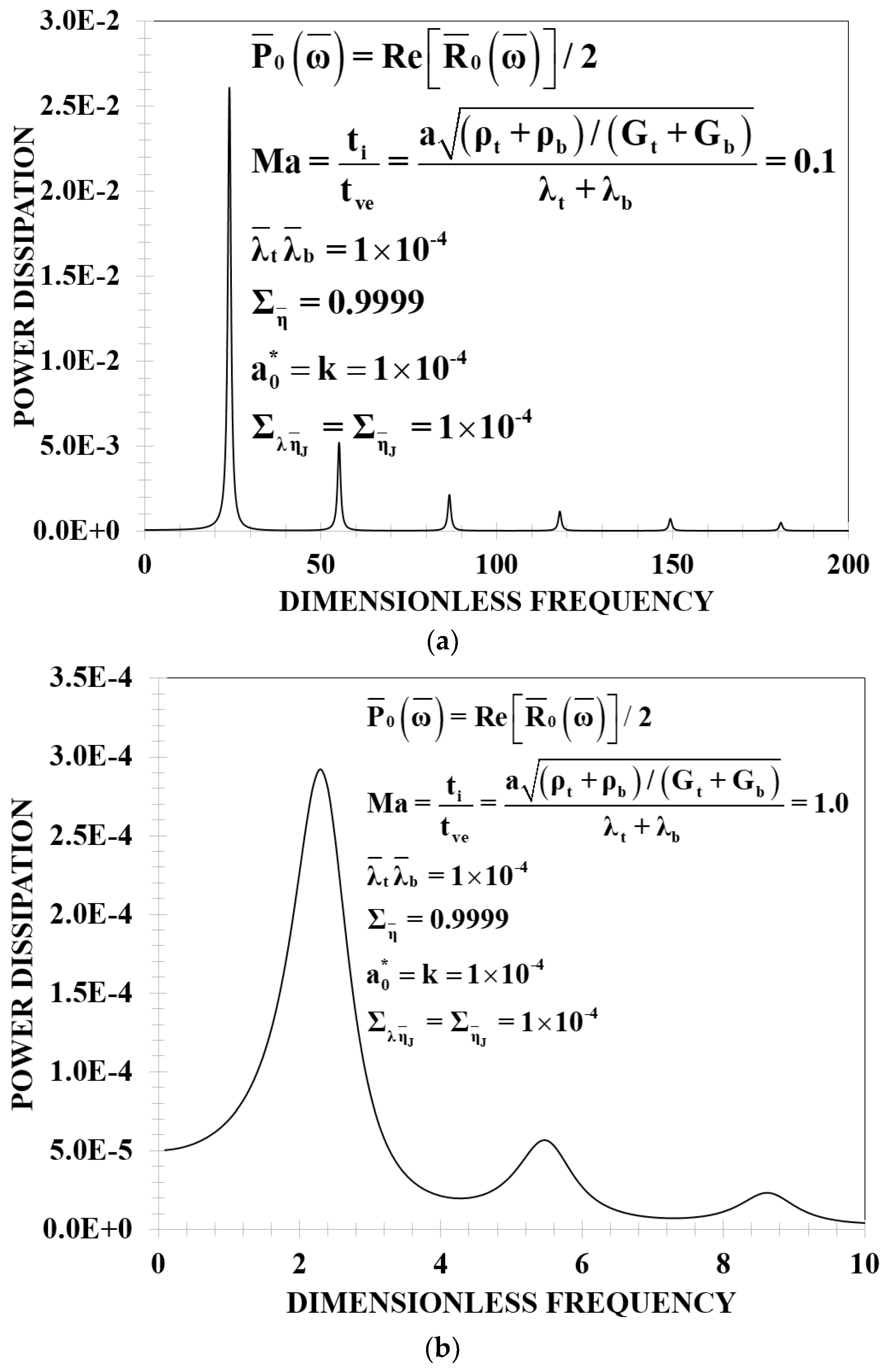
In this section, we characterize the power dissipation, and the inertia and viscoelastic mechanism are evaluated from Equations (15), (16), (20) and (21). In Figure 4a,b different resonance plots using two Ma numbers are displayed. All the numerical values of the dimensionless number correspond to the first and third modes (see Table 2).

4.2. Inertia-Viscoelastic Mechanisms: Ma ≠ 0

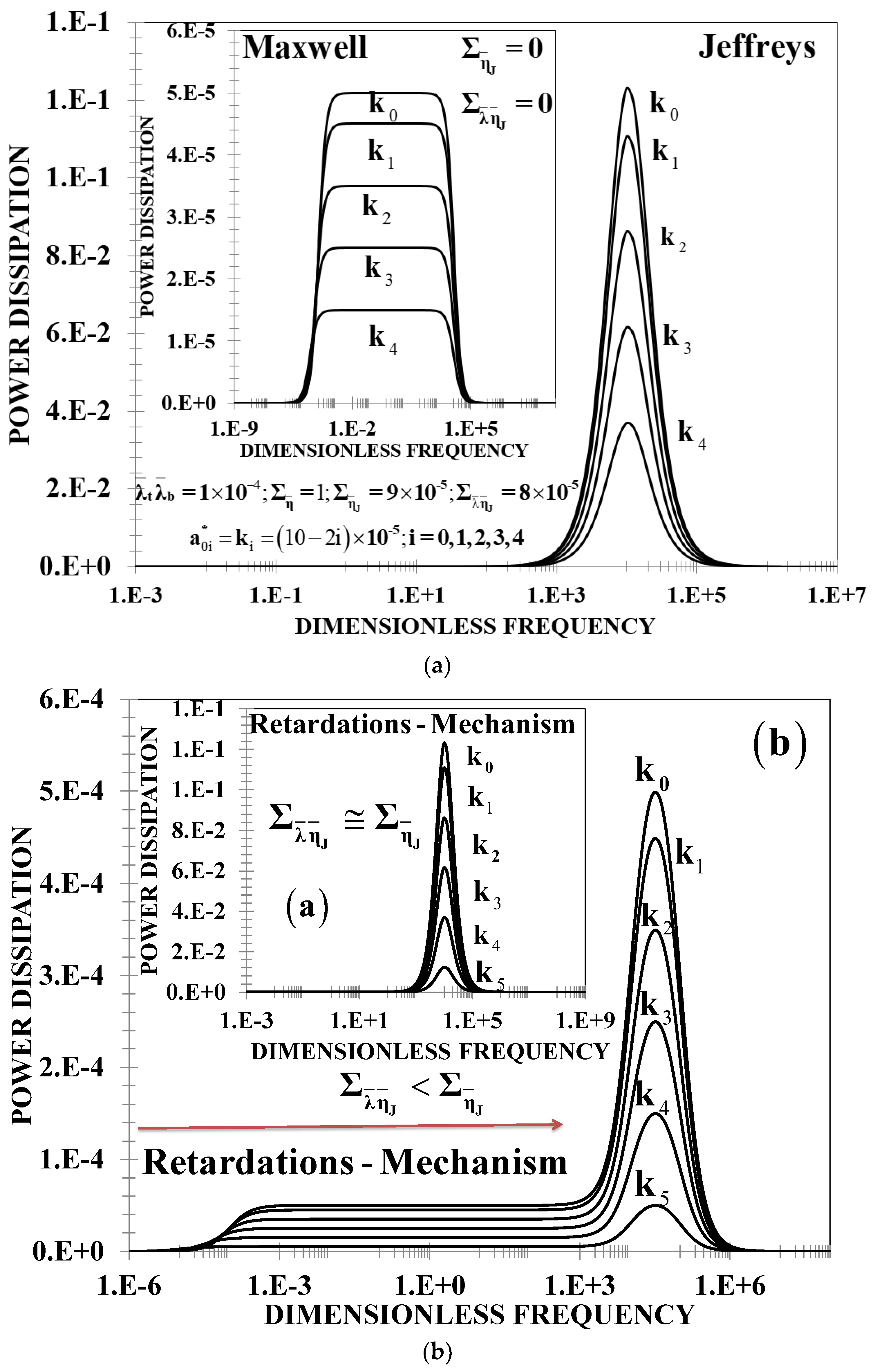
Figure 5 shows the classical resonance plots of a mechanical system similar to previous reports [12]. The effect of the resonance behavior is clearly seen through the different resonance peaks shown in Figure 5a. Here Ma = 0.1, whose value represents the viscoelastic mechanisms dominating over the inertia processes. In a previous work using up to six terms of the Bessel function expansions, the system displays only two resonance peaks [12], whereas when all the terms are considered in the transfer function, the system displays several resonance peaks, as shown in Figure 4a. With the inertial processes, the power peaks decrease, as is shown in Figure 4b. The resonance behavior is a consequence of a ratio between two Bessel functions, one of first-order and the other of zero-order, and the material properties trough the characteristic dimensionless numbers [12]. Physically, the membrane transports momentum to the viscoelastic phases associated to the viscous dissipation. The resonance peaks appear at constant intervals, but the maximum of the peak attenuates rapidly as the dimensionless frequency increases. Figure 5b shows the average membrane curvature power dissipation as a function of the dimensionless frequency. The net effect of the increase in the inertial processes is to shift the resonance curves to lower values of the dimensionless frequency, with a drastic decrease of the value of the resonance peaks in the power dissipation associated to the membrane. There is also an attenuation mechanism similar to that observed in Figure 5a. The last case, corresponding to Ma = 10, is not presented here since there is no resonance behavior in the equivalent system.

4.3. Small Mach Number: Ma << 1

In this section, the power spectrum in the case of a small Mach number, i.e., when the inertia mechanisms are smaller in comparison with viscoelastic forces is shown. In this case, the starting point of the numerical results come from Equations (16), (20), and (21). The numerical values correspond to the first and third modes of Table 2. In Figure 5, the effect of the power dissipation vs. the dimensionless frequency as a function of the retardation mechanism through the dimensionless numbers $\left\{{\mathsf{\Sigma }}_{{\overline{\mathsf{\eta }}}_{\mathrm{J}}},{\mathsf{\Sigma }}_{\overline{\mathsf{\lambda }}{\overline{\mathsf{\eta }}}_{\mathrm{J}}}\right\}$ for four particular cases corresponding to the modes {I, III} of Table 2, is shown. The mathematical and physical power predictions of the Maxwell and Jeffrey’s constitutive equations are summarized in

Table 3. Summary of the Maxwell and Jeffrey’s models’ power dissipation.

Model and Mode	Fixed Dimensionless Numbers	Viscosities Material Conditions	Material Conditions	Mathematical Description
Maxwell First Mode MI	$\begin{array}{l}{\overline{\mathsf{\lambda }}}_{\mathrm{t}}{\overline{\mathsf{\lambda }}}_{\mathrm{b}}=\mathsf{\epsilon }\\ \mathrm{k}=\mathsf{\epsilon }<<1\\ {\mathrm{a}}_0^{*}=\mathrm{k}\\ \mathsf{\epsilon }={10}^{-4}\end{array}$	$\begin{array}{l}{\mathsf{\Sigma }}_{\overline{\mathsf{\eta }}}={\left({\mathsf{\Sigma }}_{\overline{\mathsf{\eta }}}\right)}_{\min }=\mathsf{\epsilon }\\ {\mathsf{\Sigma }}_{\overline{\mathsf{\lambda }}{\overline{\mathsf{\eta }}}_{\mathrm{J}}}={\mathsf{\Sigma }}_{{\overline{\mathsf{\eta }}}_{\mathrm{J}}}=0\\ \mathsf{\epsilon }=1\times {10}^{-4}\end{array}$	1. Low symmetry 2. Small bulk viscosity 3. Floppy membrane 4. Flexoelectric mechanism of the order of LS. 5. Jeffrey’s bulk viscosities are zero	1. Constant behavior 2. Monotonically increasing behavior 3. Plateau at high frequencies Non Resonance Peak
Maxwell Third Mode MIII	$\begin{array}{l}{\overline{\mathsf{\lambda }}}_{\mathrm{t}}{\overline{\mathsf{\lambda }}}_{\mathrm{b}}=\mathsf{\epsilon }\\ \mathrm{k}=\mathsf{\epsilon }<<1\\ {\mathrm{a}}_0^{*}=\mathrm{k}\\ \mathsf{\epsilon }={10}^{-4}\end{array}$	$\begin{array}{l}{\mathsf{\Sigma }}_{\overline{\mathsf{\eta }}}={\left({\mathsf{\Sigma }}_{\overline{\mathsf{\eta }}}\right)}_{\max }=1-\mathsf{\epsilon }\\ {\mathsf{\Sigma }}_{\overline{\mathsf{\lambda }}{\overline{\mathsf{\eta }}}_{\mathrm{J}}}={\mathsf{\Sigma }}_{{\overline{\mathsf{\eta }}}_{\mathrm{J}}}=0\\ \mathsf{\epsilon }=1\times {10}^{-4}\end{array}$	1. Low symmetry 2. Large bulk viscosity 3. Floppy membrane 4. Flexoelectric mechanism of the order of LS. 5. Jeffrey’s bulk viscosities are zero	Resonance Peak
Jeffreys First Mode JI	$\begin{array}{l}{\overline{\mathsf{\lambda }}}_{\mathrm{t}}{\overline{\mathsf{\lambda }}}_{\mathrm{b}}=\mathsf{\epsilon }=1\times {10}^{-4}\\ \mathrm{k}=\mathsf{\epsilon }<<1\\ {\mathrm{a}}_0^{*}=\mathrm{k}\end{array}$	$\begin{array}{l}{\mathsf{\Sigma }}_{\overline{\mathsf{\eta }}}={\left({\mathsf{\Sigma }}_{\overline{\mathsf{\eta }}}\right)}_{\min }=\mathsf{\epsilon }\\ {\mathsf{\Sigma }}_{\overline{\mathsf{\lambda }}{\overline{\mathsf{\eta }}}_{\mathrm{J}}}\approx {\mathsf{\Sigma }}_{{\overline{\mathsf{\eta }}}_{\mathrm{J}}}\simeq \mathsf{\epsilon }\\ \mathsf{\epsilon }=1\times {10}^{-4}\end{array}$	1. Low symmetry 2. Small bulk viscosity 3. Floppy membrane 4. Jeffrey’s viscosities of the same order of the minimum bulk viscosity.	Non-monotonically behavior Maximum and Minimum
Jeffreys Third Mode JIII	$\begin{array}{l}{\overline{\mathsf{\lambda }}}_{\mathrm{t}}{\overline{\mathsf{\lambda }}}_{\mathrm{b}}=\mathsf{\epsilon }=1\times {10}^{-4}\\ \mathrm{k}=\mathsf{\epsilon }<<1\\ {\mathrm{a}}_0^{*}=\mathrm{k}\end{array}$	$\begin{array}{l}{\mathsf{\Sigma }}_{\overline{\mathsf{\eta }}}={\left({\mathsf{\Sigma }}_{\overline{\mathsf{\eta }}}\right)}_{\max }=1-\mathsf{\epsilon }\\ {\mathsf{\Sigma }}_{\overline{\mathsf{\lambda }}{\overline{\mathsf{\eta }}}_{\mathrm{J}}}\cong {\mathsf{\Sigma }}_{{\overline{\mathsf{\eta }}}_{\mathrm{J}}}=\mathsf{\epsilon }\end{array}$	1. Low symmetry 2. Small bulk viscosity 3. Floppy membrane 4. Flexoelectric mechanism of the order of LS. 5. Jeffrey’s bulk viscosities are different from zero.	1. Constant behavior 2. Monotonically increasing behavior 3. Plateau at high frequencies Non Resonance Peak

.

In all cases contained in Table 3, at lower values of the dimensionless frequency, the value of the power dissipation is close to zero. However, for a critical value of the dimensionless frequencies the system shows a monotonically-increasing behavior followed b: (i) a plateau; (ii) a resonance peak; or (iii) a non-monotonic behavior. The non-monotonic behavior of the power dissipation (maximum and minimum) can be obtained by moving the system from point J_I through the following parametric material’s conditions: (i) large asymmetry between the viscoelastic phases (one of them is weakly elastic and the other one completely viscoelastic); (ii) minimum total bulk viscosity, i.e., $\min \left\{{\mathsf{\Sigma }}_{\overline{\mathsf{\eta }}}\right\}=\mathsf{\epsilon }={10}^{-4}$; (iii) small elasticity k << 1, i.e., the elasticity of the membrane is small in comparison with the total bulk elasticity in the system ${\mathsf{\Sigma }}_{\overline{\mathrm{G}}}$; (iv) and the flexoelectric mechanisms are of the same order as the elastic ratio, i.e., ${\mathrm{a}}_0^{*}=\mathrm{k}<<1$. The mathematical condition to reach the maximum and minimum is given when the maximum values of the retardation mechanisms are equal to the minimum value of the total bulk viscosity, i.e., $\max \left\{{\mathsf{\Sigma }}_{\overline{\mathsf{\lambda }}}{}_{{\overline{\mathsf{\eta }}}_{\mathrm{J}}}\right\}=\max \left\{{\mathsf{\Sigma }}_{{\overline{\mathsf{\eta }}}_{\mathrm{J}}}\right\}\cong \min \left\{{\mathsf{\Sigma }}_{\overline{\mathsf{\eta }}}\right\}$. Physically, the bulk viscosities must satisfy the following inequality: ${\mathsf{\Sigma }}_{\mathsf{\lambda }}{}_{{\overline{\mathsf{\eta }}}_{\mathrm{J}}}\le {\mathsf{\Sigma }}_{{\overline{\mathsf{\eta }}}_{\mathrm{J}}}\le {\mathsf{\Sigma }}_{\overline{\mathsf{\eta }}}$. The bulk viscosity can be larger (close to unit) and smaller or equal to the minimum value of the relaxation times product, i.e., ${\mathsf{\Sigma }}_{\overline{\mathsf{\eta }}\min }=\min \left\{{\overline{\mathsf{\lambda }}}_{\mathrm{t}},{\overline{\mathsf{\lambda }}}_{\mathrm{b}}\right\}\simeq \mathsf{\epsilon }$. The largest asymmetry of the viscoelastic phases implies that the value of the Maxwell times ${\overline{\mathsf{\lambda }}}_{\mathrm{t}}{\overline{\mathsf{\lambda }}}_{\mathrm{b}}$ is equal to a small parameter (epsilon), i.e., ${\overline{\mathsf{\lambda }}}_{\mathrm{t}}{\overline{\mathsf{\lambda }}}_{\mathrm{b}}=\mathsf{\epsilon }$, so the minimum and maximum values of the product of the viscoelastic Maxwell times are given by: ${\overline{\mathsf{\lambda }}}_{\mathrm{t}}{\overline{\mathsf{\lambda }}}_{\mathrm{b}}=\mathsf{\epsilon }\Rightarrow \min \left\{{\overline{\mathsf{\lambda }}}_{\mathrm{t}}{\overline{\mathsf{\lambda }}}_{\mathrm{b}}\right\}=\mathsf{\epsilon },\max \left\{{\overline{\mathsf{\lambda }}}_{\mathrm{t}}{\overline{\mathsf{\lambda }}}_{\mathrm{b}}\right\}=1-\mathsf{\epsilon }$, so the new Jeffrey’s viscosities $\left\{{\mathsf{\Sigma }}_{\overline{\mathsf{\lambda }}}{}_{{\overline{\mathsf{\eta }}}_{\mathrm{J}}},{\mathsf{\Sigma }}_{{\overline{\mathsf{\eta }}}_{\mathrm{J}}}\right\}$ satisfy the next inequality:

$${\mathsf{\epsilon }\mathrm{r}}_{\mathrm{t}}{\overline{\mathsf{\eta }}}_{\mathrm{t}}+\left(1-\mathsf{\epsilon }\right){\mathrm{r}}_{\mathrm{b}}{\overline{\mathsf{\eta }}}_{\mathrm{b}}{=\mathsf{\Sigma }}_{\mathsf{\lambda }{\overline{\mathsf{\eta }}}_{\mathrm{J}}}\le {\mathsf{\Sigma }}_{{\overline{\mathsf{\eta }}}_{\mathrm{J}}}{=\mathrm{r}}_{\mathrm{t}}{\overline{\mathsf{\eta }}}_{\mathrm{t}}{+\mathrm{r}}_{\mathrm{b}}{\overline{\mathsf{\eta }}}_{\mathrm{b}}$$

(22)

In order to have the monotonic behavior of the power dissipation, both Jeffrey’s solvent and polymer viscosities must be essentially the same. The only possibility to have this mathematical condition is that one of the solvent viscosities of the Jeffrey’s model must be negligible in comparison with the other solvent viscosity associated to the other phase, so the inequality is given by:

$${\mathrm{r}}_{\mathrm{b}}{\overline{\mathsf{\eta }}}_{\mathrm{b}}\cong {\mathsf{\epsilon }\mathrm{r}}_{\mathrm{t}}{\overline{\mathsf{\eta }}}_{\mathrm{t}}+\left(1-\mathsf{\epsilon }\right){\mathrm{r}}_{\mathrm{b}}{\overline{\mathsf{\eta }}}_{\mathrm{b}}={\mathsf{\Sigma }}_{\mathsf{\lambda }{\overline{\mathsf{\eta }}}_{\mathrm{J}}}\le {\mathsf{\Sigma }}_{{\overline{\mathsf{\eta }}}_{\mathrm{J}}}{=\mathrm{r}}_{\mathrm{t}}{\overline{\mathsf{\eta }}}_{\mathrm{t}}{+\mathrm{r}}_{\mathrm{b}}{\overline{\mathsf{\eta }}}_{\mathrm{b}}\cong {\mathrm{r}}_{\mathrm{b}}{\overline{\mathsf{\eta }}}_{\mathrm{b}}$$

(23)

The only possibility to fulfill the equality (Equation (23)) is when the product between the viscosity ratio r_t value becomes very small. Physically, the above condition implies that the solvent and polymer viscosities play an important role in the dynamical behavior of the Jeffrey’s model. As a first partial conclusion, in the Maxwell model (2ODE) the resonance behavior is reached in the third mode [10,12], whereas in the Jeffress model (3ODE), the resonance behavior with the maximum and minimum is reached in mode I.

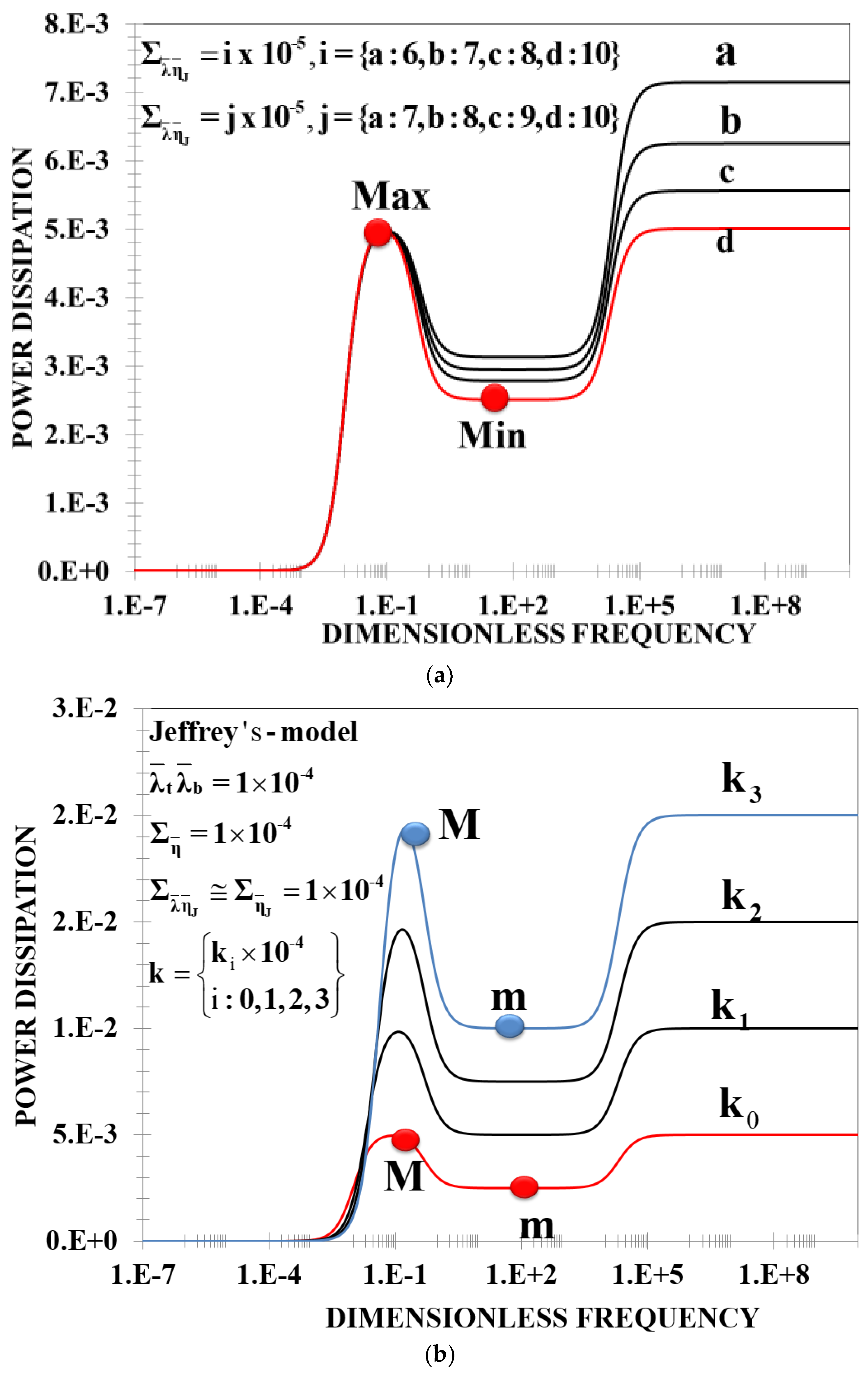
For the fourth curves showed in Figure 5, the power dissipation is negligible at low frequencies up to a critical dimensionless frequency where the power dissipation shows a monotonically-increasing behavior until a maximum, followed by a decreasing behavior, followed by a plateau zone at intermediate frequencies. For a second critical value of the dimensionless frequency, the system experinces a monotonically-increasing behavior followed by a second plateau at high frequencies, whose value depends on the elastic properties of the membrane. It is important to note that, when the retardation viscosities satisfy the following inequality ${\mathsf{\Sigma }}_{\mathsf{\lambda }{\overline{\mathsf{\eta }}}_{\mathrm{J}}}<{\mathsf{\Sigma }}_{{\overline{\mathsf{\eta }}}_{\mathrm{J}}}\ne 0$, the value of the power dissipation plateau at high dimensionless frequency is greater than the local maximum and its value depends on the elastic dimensionless ratio and the retardation viscosity. Notice that when the values of the retardation viscosities are of the same order, i.e., ${\mathsf{\Sigma }}_{\mathsf{\lambda }{\overline{\mathsf{\eta }}}_{\mathrm{J}}}\cong {\mathsf{\Sigma }}_{{\overline{\mathsf{\eta }}}_{\mathrm{J}}}$ the numerical value of the local maximum power dissipation and the plateau at high dimensionless frequency are of the same order. The retardation mechanisms play an important role in the description of the non-monotonically behavior described by other authors with different electro-mechanical approaches [15].

In Figure 6, the power dissipation as a function of the dimensionless frequency is displayed for the Jeffreys model using Equations (20) and (21) as a function of the elastic mechanism. In the inset, the results for the Maxwell model are shown [10,12]. For a critical value of the resonance frequency the Jeffrey’s model displays a well-localized resonance behavior, which is a decreasing function of the elastic dimensionless number k. The maximum amplitude of the power is related to the high fluid asymmetry ${\overline{\mathsf{\lambda }}}_{\mathrm{t}}{\overline{\mathsf{\lambda }}}_{\mathrm{b}}<<1$ (essentially a viscous liquid and a viscoelastic liquid), large viscosity ${\mathsf{\Sigma }}_{\overline{\mathsf{\eta }}}\to 1$ (maximum dissipation), small elastic ratio k << 1 and high retardation fluids asymmetry, ${\mathsf{\Sigma }}_{\overline{\mathsf{\lambda }}}{}_{{\overline{\mathsf{\eta }}}_{\mathrm{J}}}\cong {\mathsf{\Sigma }}_{{\overline{\mathsf{\eta }}}_{\mathrm{J}}}$, which basically means that one of the retardation times is smaller in comparison to the other one. This fact arises because the retardation mechanisms are not independent of the Maxwell relaxation times and are linked by a ratio between the solvent and polymer viscosity of the Jeffrey’s model. For the Maxwell model, a resonance behavior was found, where the value of the peak amplitude is determined by the elastic ratio [10,12]: ${\overline{\mathrm{p}}}_{\mathrm{peak}}=\mathrm{k}\left(1-\mathrm{k}\right)/2$. This equation shows a quadratic dependence with the elastic ratio and its maximum value of the power peak dissipation is obtained for $\mathrm{k}=1/2$ and it is given by ${\overline{\mathrm{p}}}_{\mathrm{peak}-\max }\left(\mathrm{k}=1/2\right)=1/8$ [25,32]. However, there is a difference in the frequency “width” of the power pulse, with wider pulses for lower k values.

Figure 7 shows the power dissipation vs. the dimensionless frequency as a function of the elastic ratio k, for two different cases of the retardation numbers: (a) ${\mathsf{\Sigma }}_{\overline{\mathsf{\lambda }}{\overline{\mathsf{\eta }}}_{\mathrm{J}}}={\mathsf{\Sigma }}_{{\overline{\mathsf{\eta }}}_{\mathrm{J}}}$ and (b) ${\mathsf{\Sigma }}_{\overline{\mathsf{\lambda }}{\overline{\mathsf{\eta }}}_{\mathrm{J}}}<{\mathsf{\Sigma }}_{{\overline{\mathsf{\eta }}}_{\mathrm{J}}}$. The main effect of the retardation mechanism is to shift the resonance peak to higher values of the dimensionless frequencies and increase the power peak maximum.

5. Discussion

5.1. Biological Applications

As demonstrated elsewhere [1,2,3,6,7,8,9,10,18,19,20,21], a key biological feature is the shape and location of the power amplification pulse [18,19,20,21]. In our flexoelectric model, the non-monotonic behavior of the power associated with its maximum (resonance) and minimum (anti-resonance) emerges under the following material conditions: (i) asymmetric of the phases ${\overline{\mathsf{\lambda }}}_{\mathrm{t}}{\overline{\mathsf{\lambda }}}_{\mathrm{b}}=\mathsf{\epsilon }<<1$, (ii) small bulk-viscous mechanism $\min \left\{{\mathsf{\Sigma }}_{\overline{\mathsf{\eta }}}\right\}=\mathsf{\epsilon }$, (iii) small elastic ratio $\mathrm{k}<<1$ and, (iv) the retardation mechanism are almost equal and their values are close to the minimum value of the bulk viscosity, i.e., $\max \left\{{\mathsf{\Sigma }}_{\overline{\mathsf{\lambda }}{\overline{\mathsf{\eta }}}_{\mathrm{J}}}\right\}\cong \min \left\{{\mathsf{\Sigma }}_{{\overline{\mathsf{\eta }}}_{\mathrm{J}}}\right\}=\mathsf{\epsilon }<<1$. The above material conditions imply that the ratio between the solvent and polymer viscosities in one of the viscoelastic phases must be of the order of the main value of the bulk viscosity i.e., ${\mathrm{r}}_{\mathrm{b}}={\mathsf{\eta }}_{\mathrm{s}\mathrm{b}}/{\mathsf{\eta }}_{\mathrm{s}\mathrm{b}}+{\mathsf{\eta }}_{\mathrm{p}\mathrm{b}}=\mathsf{\epsilon }$. Physically, the system decreases the dissipation mechanism until its minimum value is reached and the retardation mechanics maximizes it. Rabbits et al. [15] employed an electromechanical system in which the non-monotonically behavior depends on the material properties in the system and the length of the Outer Hair Cells (see [15], Figure 7). In our 3ODE membratodynamic model the geometry and flexoelectric properties are contained in the dimensionless number ${\mathrm{a}}_0^{*}$ which is of the order of the elastic ratio k, i.e., ${\mathrm{a}}_0^{*}=\mathrm{k}<<1$ [10,12].

5.2. Material Properties and Resonance Conditions

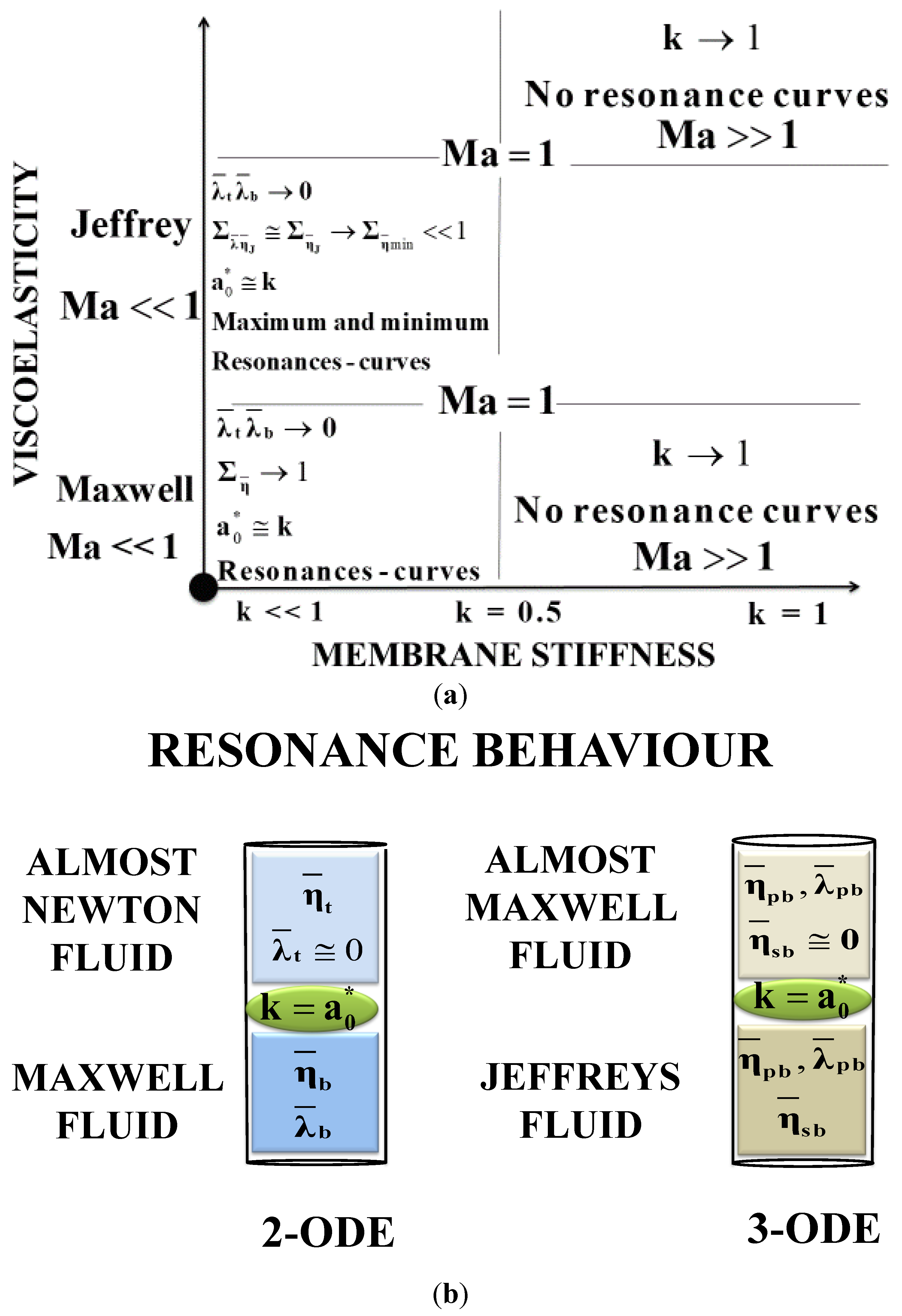
The resonant and anti-resonant behaviors of the power dissipation are characterizing aspects of the OHC cells [15]. The material parameters of importance are: (i) Maxwell relaxation times; (ii) bulk elasticity of the viscoelastic phases; (iii) polymer viscosities; (iv) elastic membrane energy; and (v) solvent viscosities. The specific ways to adapt these parameters are by changing the concentration and the molecular weight distribution of dissolved polymer chains [10,12]. To have the non-monotonic behavior (maximum and minimum) and the power amplitude, one of the liquid phases must be weakly elastic and the other one completely viscoelastic (phase asymmetry) [10,12]. To shift the position of the localized power plateau and width of the power plateau, the elasticity of the membrane with respect to the bulk (viscoelastic phases) must be tuned (see Figure 7a,b). To widen the power plateau, the Maxwell relaxation times, elasticity of the membrane, and viscoelastic phases must be modified [10,12]. Combining the results from Figure 5, Figure 6 and Figure 7 we can arrive at a complementary qualitative picture of power delivery for the Jeffreys and Maxwell model as a function of the membrane stiffness through the elastic ratio k (Figure 8a,b).

6. Conclusions

In this paper we explored the dynamics of the actuation flexoelectric mode [1,2,6,7,8]. Using the flexoelectric shape equation in conjunction with a viscoelastic capillary flow model for the contacting phases, a new average curvature dynamic was obtained (Equations (12) and (13)). The third-order model for the electric field (input) and curvature or volumetric flow (output) is given by a balance of retardation, inertial, viscous, and elastic effects, originating from the flexoelectric membrane and the viscoelastic Jeffreys fluids (solvent and polymer mechanisms). Moreover, this new model (3ODE) can be interpreted as the sum of a second-order ordinary differential equation plus a small perturbation, which it is associated with retardation mechanisms. These third-order models are well known and they are associated to the jerk-force mechanism (timed derivative of acceleration) in ODEs, chaotic systems, and classic Newtonian mechanics [34]. When the retardation mechanisms are zero, i.e., ${\overline{\mathsf{\lambda }}}_{\mathrm{J}\mathrm{i}}=0;\mathrm{i}=\left\{\mathrm{t},\mathrm{b}\right\}$, the previous Maxwell model is recovered with inertial and inertialess mechanisms [10,12]. Using dimensionless variables, and taking into account the inertia mechanisms in the system, the physics can be described with seven dimensionless numbers (Equations (11) and (21)). These dimensionless numbers are associated with the inertia, retardation, memory, viscous, elastic membrane, and flexoelectric mechanisms. A thorough parametric study was performed to identify the conditions that lead to the appearance of a maximum (resonance behavior) or a minimum (anti-resonance behavior) in the power spectrum (Table 3). The maximum and minimum are found in mode I (Figure 5), when the system presents a: (i) large asymmetry between the viscoelastic phases (one on phases is weakly elastic and the other one completely viscoelastic); (ii) minimum total bulk viscosity; (iii) small elasticity; and (iv) the flexoelectric mechanisms are of the order of the elasticity of the membrane [10,12]. The mathematical condition to reach the maximum and minimum are given when the maximum values of the retardation mechanisms are equal to the minimum value of the dissipation energy, i.e., $\max \left\{{\mathsf{\Sigma }}_{\overline{\mathsf{\lambda }}}{}_{{\overline{\mathsf{\eta }}}_{\mathrm{J}}}\right\}\cong \max \left\{{\mathsf{\Sigma }}_{{\overline{\mathsf{\eta }}}_{\mathrm{J}}}\right\}\simeq \min \left\{{\mathsf{\Sigma }}_{\overline{\mathsf{\eta }}}\right\}=\mathsf{\epsilon }={10}^{-4}$. The above mathematical condition implies that the solvent and polymer viscosities play an important role in the resonance and anti-resonance behaviour (Figure 6a,b). Physically, this means that in order to get a non-monotonically increasing behavior, a contrast in the liquid phases is necessary with one of them being weakly elastic and the other one being highly viscoelastic (Equations (22) and (23)). For example, if one of the viscoelastic phases is characterized by the Jeffrey’s or Maxwell model, the other one must be represented by the Maxwell or the Newtonian constitutive equation, respectively. It is important to note that the Maxwell and Jeffrey’s times are not independent and they satisfy a linear relation, whose slope is given by a ratio between the solvent viscosity and the polymer contribution to the bulk viscosity (Section 2). The non-monotonically behaviour has been reported using a mechano-electrical model as a consequence of the outer hair cell length [15] (see [15], Figure 7b). In constrast, the lector-rheological model used here, showed that the solvent and the polymer mechanisms induced a similar non-monotonic behaviour in the power dissipation as a function of the applied electrical field. Here, the maximum and minimum is controlled by coupling effects between the solvent and the polymer contributions of the liquid viscoelastic phases (Figure 6a). The numerical values of maximum and minimum is controlled by the elastic ratio k and the flexoelectric mechanisms trough the flexoelectric number ${\mathrm{a}}_0^{*}$. Notice that in order to have the maximum and minimum in the system, the flexoelectric number ${\mathrm{a}}_0^{*}$ must be of the same order as k, i.e., ${\mathrm{a}}_0^{*}=\mathrm{k}$ (Figure 6b). When the asymmetry of the viscoelastic phases increases, the power peak and the resonance width decrease and increase, respectively. These effects are shown in Figure 6 and Figure 7 and summarized in Table 3. Furthermore, optimization of the power device can be obtained by minimizing the stored elastic membrane energy and maximizing the power dissipation. This was discussed in previous works [9,10,12]. In addition, when one of the solvent contributions is small in comparison with the other solvent phase, a close expression for the power dissipation is found (small Mach number, Ma << 1, Equations (16), (20) and (21)).

Physically, the dissipation dominates over the elastic storage membrane mechanisms in the resonance behavior [9,10,12,15]. The effect of the resonance behavior through the Mach number is to display more resonant peaks which can be associated to biological processes (see the Deborah number in [10,12]). The inclusion of new rheological parameters through higher models can be done by changing the Jeffrey’s viscosity operator given in Table 1.

The merits of this research is to extend the previous theory [1,2,6,7,8,9,10,12], for any particular linear or fractional viscoelastic constitutive equation, through the generalized viscosity differential operator given in Table 1.

In particular, the Jeffreys viscosity function was chosen to include the solvent and polymer mechanisms. When the inertia is included in the system through the Mach number several resonance peaks are found, which, from a biological point of view, could be relevant (Figure 4). In the inertialess regime (Ma = 0), a third-order differential equation (3ODE) was found (Equations (10)–(12)). This electro-rheological model led to a non-monotonically decreasing behavior, which is directly related to the new viscosities associated with the retardation mechanisms, which are linked by the solvent and polymer contributions. Lastly, a qualitative evaluation of the present model predictions based on a non-monotonically power profile, indicates that the Helfrich-Flexoelectric-Jeffrey’s fluid model possesses the necessary physics to qualitatively capture the electro-mechanical power conversion phenomena. Future extensions include higher-order and fractional viscoelastic models, non-linear viscoelasticity, and mass transfer induced by shear forces [35,36]. Heat dissipation and non-linear effects due to high frequencies, compressible systems (density as a function of the pressure drop), and others diseases which can affect the hearing system (hypercholesterolemia, hyperglycemia, genetic problems, etc.) lie outside of the scope of the present research [37,38,39,40,41]. A posible path to continue this research is to exted it to new models in the regime of nonlinear viscoelasticity (large deformations). The nonlinearity induced by large deformations can be explored with two approaches. The nonlinearity comes from the flexoelectric membrane or can be induced through the viscoelastic liquid phases. These new approaches must be explored through analytical and numerical algoritms and can be a starting point of new reaserch. The present theory, model, and computations contribute to the evolving fundamental understanding of biological shape actuation through electromechanical couplings [1,2,3,4,9,10,11,12,35,36,37] involving liquid crystallinity.

References

- Rey, A.D. Liquid crystals models of biological materials and processes. Soft Matter 2010, 6, 3402–3429. [Google Scholar] [CrossRef]
- Rey, A.D. Capillary models for liquid crystal fibers, membranes, films, and drops. Soft Matter 2007, 2, 1349–1368. [Google Scholar] [CrossRef]
- Rey, A.D.; Herrera-Valencia, E.E.; Murugesan, Y.K. Structure and Dynamics of Biological Liquid Crystals. Liq. Cryst. 2013, 41, 430–451. [Google Scholar] [CrossRef]
- Rey, A.D.; Herrera-Valencia, E.E. Liquid crystal models of biological materials and silk spinning. Biopolymers 2012, 97, 374–396. [Google Scholar] [CrossRef] [PubMed]
- Rey, A.D.; Herrera-Valencia, E.E. Rheological theory and simulations of surfactant nematic liquid crystals. In Self-Assembled Supramolecular Architectures: Lyotropic Liquid Crystals; Garti, N., Somasundaran, P., Mezzenga, R., Eds.; John Wiley & Sons Inc.: Hoboken, NJ, USA, 2012. [Google Scholar]
- Petrov, A.G. The Lyotropic State of Matter: Molecular Physics and Living Matter Physics; Gordon and Breach Science Publisher: Amsterdan, The Netherlands, 1999. [Google Scholar]
- Petrov, A.G. Electricity and mechanics of biomembrane systems: Flexoelectricity in living membranes. Anal. Chim. Acta 2006, 568, 70–83. [Google Scholar] [CrossRef] [PubMed]
- Petrov, A.G. Flexoelectricity of model and living membranes. BBA-Biomembranes 2001, 1561, 1–25. [Google Scholar] [CrossRef]
- Rey, A.D. Linear Viscoelastic Model for Bending and Torsional Modes in Fluid Membranes. Rheol. Acta 2008, 47, 861–871. [Google Scholar] [CrossRef]
- Abou-Dakka, M.; Herrera-Valencia, E.E.; Rey, A.D. Linear oscillatory dynamics of flexoelectric membranes embedded in viscoelastic media with applications to outer hair cells. J. Non-Newton Fluid Mech. 2012, 185–186, 1–17. [Google Scholar] [CrossRef]
- Rey, A.D.; Servio, P.; Herrera-Valencia, E.E. Bioinspired model of mechanical energy harvesting based on flexoelectric membranes. Phys. Rev. E 2013, 87, 022505. [Google Scholar] [CrossRef] [PubMed]
- Herrera-Valencia, E.E.; Rey, A.D. Mechano-electric transduction Performance of Actuation Device based on liquid crystal Membrane Flexoelectricity. Philos. Trans. R. Soc. A 2014, 372, 20130369. [Google Scholar] [CrossRef] [PubMed]
- Rey, A.D.; Servio, P.; Herrera-Valencia, E.E. Stress-Sensor Device Based on Flexoelectric Liquid Crystalline Membranes. ChemPhysChem 2014, 15, 1405–1412. [Google Scholar] [CrossRef] [PubMed]
- Aguilar-Gutierrez, O.F.; Herrera-Valencia, A.D.; Rey, A.D. Generalized Boussinesq-Scriven surface fluid model with curvature dissipation for liquid surfaces and membranes. J. Colloid Interface Sci. 2017, 503, 103–114. [Google Scholar] [CrossRef] [PubMed]
- Rabbits, R.D.; Clifford, S.; Breneman, K.D.; Farrell, B.; Brownell, W.E. Power efficiency of outer hair cell somatic electromotility. PLoS Comput. Biol. 2009, 5, e1000444. [Google Scholar] [CrossRef]
- Sachs, F.; Brownell, W.E.; Petrov, A.G. Membrane electromechanics in biology, with a focus on hearing. MRS Bull. 2009, 34, 665–670. [Google Scholar] [CrossRef] [PubMed]
- Spector, A.A.; Deo, N.; Ratnanather, J.T.; Raphael, R.M. Electromechanical models of the outer hair cell composite membrane. J. Membr. Biol. 2006, 209, 135–152. [Google Scholar] [CrossRef] [PubMed]
- Brownell, W.E. Evoked mechanical responses of isolated cochlear outer hair cells. Science 1985, 227, 194–196. [Google Scholar] [CrossRef] [PubMed]
- Oghalai, J.S.; Zhao, H.B.; Kutz, J.W.; Brownell, W.E. Voltage-and tension-dependent lipid mobility in the outer hair cell plasma membranes. Science 2000, 287, 658–661. [Google Scholar] [CrossRef] [PubMed]
- Raphael, R.M.; Popel, A.S.; Brownell, W.E. A membrane bending model of outer hair cell electromotility. Biophys. J. 2000, 78, 2844–2862. [Google Scholar] [CrossRef]
- Hawkins, R.D.; Lovett, M. The developmental genetics of auditory hair cells. Hum. Mol. Genet. 2004, 13, R289–R296. [Google Scholar] [CrossRef] [PubMed]
- Panagopoulos, D.J.; Karabarbounis, A.; Margaritis, L.H. Mechanism for action of electromagnetic field on cells. Biochem. Biophys. Res. Commun. 2002, 298, 95–102. [Google Scholar] [CrossRef]
- Fikus, M.; Pawlowski, P. Bioelectrorheolgical model of the cell. 2. Analysis of creep and its experimental verification. J. Theor. Biol. 1989, 37, 365–373. [Google Scholar] [CrossRef]
- Ehrenstein, D.; Iwasa, K.H. Viscoelastic relaxation in the membrane of the auditory outer hair cell. J. Biophys 1996, 71, 1087–1094. [Google Scholar] [CrossRef]
- Ren, T.; He, W.; Barr-Gillespie, P.G. Reverse transduction measured in the living cochlea by low-coherence heterodyne interferometry. Nat. Commun. 2016, 7, 10282. [Google Scholar] [CrossRef] [PubMed]
- Iwasa, K.H. Negative membrane capacitance of outer hair cells: Electromechanical coupling near resonance. Sci. Rep. 2017, 7, 12118. [Google Scholar] [CrossRef] [PubMed]
- Ren, T.; He, W.; Li, Y.; Grosh, K.; Fridberger, A. Light-induced vibration in the hearing organ. Sci. Rep. 2014, 4, 5941. [Google Scholar] [CrossRef] [PubMed]
- Ospeck, M.; Iwasa, K.H. How to close should the outer hair cell RC roll-off frequency be to characteristic frequency? Biophys. J. 2012, 102, 1767–1774. [Google Scholar] [CrossRef] [PubMed]
- Wang, Y.; Steele, C.R.; Puria, S. Cochlear outer-hair-cell power generation and viscous fluid loss. Sci. Rep. 2016, 6, 19475. [Google Scholar] [CrossRef] [PubMed]
- Nam, J.H.; Peng, A.W.; Ricci, A.J. Underestimated sensitivity of mammalian cochlear hair cells due to splay between stereociliary columns. Biophys. J. 2015, 108, 2633–2647. [Google Scholar] [CrossRef] [PubMed]
- Maoiléidigh, D.O.; Jülicher, F. The interplay between active hair bundle motility and electromotility in the cochlea. J. Acoust. Soc. Am. 2010, 128, 1175–1190. [Google Scholar] [CrossRef] [PubMed]
- Iwasa, K.H.; Sul, B. Effect of the cochlear microphonic on the limiting frequency of the mammalian ear. J. Acoust. Soc. Am. 2008, 124, 1607–1612. [Google Scholar] [CrossRef] [PubMed]
- Iwasa, K.H. Effect of stress on the membrane capacitance of the auditory outer hair cell. Biophys. J. 1993, 65, 492–498. [Google Scholar] [CrossRef]
- Sprott, J.C. Some simple chaotic jerk functions. Am. J. Phys. 1997, 65, 537–543. [Google Scholar] [CrossRef]
- Forest, M.G.; Wang, Q.; Zhou, R. Kinetic theory and simulations of active polar liquid crystalline polymers. Soft Matter 2013, 9, 5207–5222. [Google Scholar] [CrossRef]
- Grecov, D.; Rey, A.D. Theoretical and computational rheology for discotic nematic liquid crystals. Mol. Cryst. Liq. Cryst. 2003, 39, 57–94. [Google Scholar] [CrossRef]
- Herrera-Valencia, E.E.; Calderas, F.; Medina-Torres, L.; Pérez Camacho, M.; Moreno, L.; Manero, O. On the pulsating flow behavior of a biological fluid: Human blood. Rheol. Acta 2017, 56, 387–407. [Google Scholar] [CrossRef]
- Herrera-Valencia, E.E.; Sánchez-Villavicencio, M.L.; Calderas, F.; Pérez Camacho, M.; Medina-Torres, L. Simultaneous pulsatile flow and oscillating wall of a non-Newtonian liquid. Korea-Aust. Rheol. Acta 2016, 28, 281–300. [Google Scholar] [CrossRef]
- Herrera-Valencia, E.E.; Calderas, F.; Chávez, A.E.; Manero, O. Study on the pulsating flow of a worm-like micellar solution. J. Non-Newtonian Fluid Mech. 2010, 165, 174–183. [Google Scholar] [CrossRef]
- Herrera-Valencia, E.E.; Calderas, F.; Chávez, A.E.; Manero, O.; Mena, B. Effect of random longitudinal vibrations pipe on the Poiseuille flow of pulsating flow of a complex liquid. Rheol. Acta 2009, 48, 779–800. [Google Scholar] [CrossRef]
- Sánchez-Villavicencio, M.L.; Vinqvist-Tychuk, M.; Kalt, W.; Matar, C.; Alarcón Aguilar, F.J.; Escobar Villanueva, M.C.; Haddad, P.S. Fermented blueberry juice extract and its specific fractions have an anti-adipogenic effect in 3 T3-L1 cells. BMC Complement. Altern. Med. 2017, 17, 24. [Google Scholar] [CrossRef] [PubMed]
Figure 1.
Flow chart of the paper’s organization. Ma denotes the Mach number.
Figure 2.
Schematic of the geometry and operation of flexoelectric mechanics, defined in a capillary geometry of radius r = a, and axial length L. The input E field distorts the initially flat circular membrane into a spherical cap of radius R and height h. The flexoelectric actuation creates a capillary viscoelastic flow in the contacting top (t) and bottom (b) fluids of viscosities {ηt,ηb}, relaxation times {λt, λb}, retardation times {λJt, λJb} and fluid densities {ρt, ρb}. Adapted from references [10,12], where M was defined as: .
Figure 3.
Prismatic material space for the six possible modes of Equation (16), shown in Table 1. The vertical axis is the memory, the horizontal is the elasticity ratio k, and the axis out of the page plane is the total viscosity. The six vertices correspond to the six modes in Table 2. Below the prism, the horizontal arrow shows the range of the dimensional numbers: (i) memory , (ii) Maxwell relaxation numbers , (iii) total bulk viscosity , (iv) Bulk retardation viscosity , and (v) bulk weighted retardation viscosity . The triangle in the upper right corner describes the material line that contains the modes corresponding to a small elasticity ratio where the power dissipation is different form zero. The line I–III shows the material conditions where the model displays a monotonical behavior (mode III) and non-monotonical solvent behavior (mode I).
Figure 4.
Power dissipation of the membrane curvature vs dimensionless frequency for different inertial conditions. Figure 4 (a,b) show the effect of two Mach number conditions: (a) Ma = 0.1, (b) Ma = 1. The other parameters employed in the simulation correspond to the third mode and the numerical Jeffrey’s viscosities are approximately of the same order of magnitude.
Figure 5.
(a) Power as a function of the dimensionless frequency for the four cases depicted in Table 2. The maximum and minimum are clearly seen in simulation J1 (first mode). The cases M1 and J2 show a similar monotonically-increasing behavior followed by a plateau. The last case, M2, shows a typical resonance curve in mode III. (b) Power resonances for the Maxwell and Jeffrey’s models corresponding to the first and third modes of Table 3.
Figure 6.
(a) Power dissipation as a function of the dimensionless frequency for different values of the elastic ratio k and the dimensionless Jeffreys viscosities. Here the Mach number is zero. Figure 7a instead of Figure 6a (Maxwell model). In (b) the Jeffreys model for two different Jeffrey´s viscosities material conditions. The other material parameters used in the simulaion are the same as in Figure 7a.
Figure 7.
(a) Power dissipation as a function of the dimensionless frequency for different values of the dimensionless Jeffreys viscosities. (b) Power dissipation as a function of the dimensionless frequency for different values of the elastic membrane ratio. The material properties used in the simulation correspond to mode III. Softer membranes generate greater power dissipation.
Figure 8.
(a) Schematic viscoelastic mechanisms as a function of the elastic ratio k, for the Jeffrey’s (top) and Maxwell (bottom) models, respectively. The four quadrants in each case represent performance conditions most likely to be relevant to biological flexoelectric membranes. In (b) a qualitative schematic of the material conditions for resonance is shown. For the Maxwell system one of the viscoelastic phases must be almost inelastic, whereas in the Jeffreys system one of the viscoelastic phases must be almost a Maxwell-like fluid.