Leaky Flow through Simplified Physical Models of Bristled Wings of Tiny Insects during Clap and Fling


School of Mechanical and Aerospace Engineering, Oklahoma State University, 218 Engineering North, Stillwater, OK 74078-5016, USA
*
Author to whom correspondence should be addressed.
Fluids 2018, 3(2), 44; https://doi.org/10.3390/fluids3020044
Submission received: 30 March 2018
/
Revised: 31 May 2018
/
Accepted: 13 June 2018
/
Published: 19 June 2018
(This article belongs to the Special Issue Bio-inspired Flow)
Abstract
:In contrast to larger flight-capable insects such as hawk moths and fruit flies, miniature flying insects such as thrips show the obligatory use of wing–wing interaction via “clap and fling” during the end of upstroke and start of downstroke. Although fling can augment lift generated during flapping flight at chord-based Reynolds number () of 10 or lower, large drag forces are necessary to clap and fling the wings. In this context, bristles observed in the wings of most tiny insects have been shown to lower drag force generated in clap and fling. However, the fluid dynamic mechanism underlying drag reduction by bristled wings and the impact of bristles on lift generated via clap and fling remain unclear. We used a dynamically scaled robotic model to examine the forces and flow structures generated during clap and fling of: three bristled wing pairs with varying inter-bristle spacing, and a geometrically equivalent solid wing pair. In contrast to the solid wing pair, reverse flow through the gaps between the bristles was observed throughout clap and fling, resulting in: (a) drag reduction; and (b) weaker and diffuse leading edge vortices that lowered lift. Shear layers were formed around the bristles when interacting bristled wing pairs underwent clap and fling motion. These shear layers lowered leakiness of flow through the bristles and minimized loss of lift in bristled wings. Compared to the solid wing, peak drag coefficients were reduced by 50–90% in bristled wings. In contrast, peak lift coefficients of bristled wings were only reduced by 35–60% from those of the solid wing. Our results suggest that the bristled wings can provide unique aerodynamic benefits via increasing lift to drag ratio during clap and fling for between 5 and 15.
1. Introduction
Miniature flying insects with body lengths less than 1 mm, such as thrips, fairyflies, and some parasitoid wasps, have to contend with generating lift in the face of large viscous resistance at chord-based Reynolds number () on the order of 10 or lower [1]. In contrast to our understanding of the aerodynamics of insect flight at the scale of fruit flies and above [2,3,4,5,6,7], the fluid dynamic mechanisms that enable the smallest flying insects to generate lift remain unclear. At low ∼(10), drag forces substantially peak and hinder aerodynamic performance [8,9]. Tiny insects show two distinct physical adaptations when compared to larger insects such as fruit flies and hawk moths, including: (1) obligatory use of “clap and fling” wing–wing interaction as a part of free-flight wingbeat kinematics [10,11,12]; and (2) wings consisting of a thin solid membrane with long bristles on the fringes. Recent studies by Santhanakrishnan et al. [13] and Jones et al. [14] have proposed that bristled wings can reduce drag forces needed to fling wings apart at low . However, the physical mechanisms underlying drag reduction by bristled wings and the impact of bristles on lift generation via clap and fling have not been previously examined. It is unclear whether unique aerodynamic advantages are associated with the marked preference in bristled wings among the smallest flying insects.
For insects that fly at ranging (100) to (1000), such as fruit flies, honeybees, and hawk moths, dynamic stall has been shown to be an important unsteady mechanism of lift generation [15,16]. Flapping at large angles of attack results in separation of flow at the sharp leading edge, culminating in the formation of an attached leading edge vortex (LEV) and a trailing edge vortex (TEV) that is shed into the wake. Throughout the duration of a stroke, the LEV is stably attached to the top surface of the wing and is shed in the wake at the end of the stroke [16]. The presence of an attached LEV increases the lift force produced by flapping, by effecting a beneficial alteration of the streamwise pressure gradient and increasing both the steady-state as well as instantaneous circulation over the wing. Hovering insects tune their wing kinematics to delay or suppress LEV shedding and circumvent the possibility of stall [16,17,18]. However, lift generation using dynamic stall is challenged for ∼(10) due to formation of an attached LEV and an attached TEV [9]. This “vortical symmetry” was shown to lower lift forces during single wing translation [9]. It is thus unlikely that lift generated during flapping translation [2] can sustain long-distance migration reported in thrips [19]. Although passive dispersal and intermittent parachuting [13] can lower the energetic demands of migrating thrips, active flight activity of thrips has been reported in blueberry fields as large as 3000 square metres [20].
Previous hypotheses proposed for lift generation by the smallest flying insects have focused on: (i) asymmetry in upstroke and downstroke; and (ii) wing–wing interaction via clap and fling between end of upstroke and start of downstroke. Horridge et al. [21] suggested that tiny insects could modulate the instantaneous angle of attack, so that most of the lift is generated during the downstroke and negative lift is minimized during the upstroke. However, the LEV-TEV symmetry observed during single wing translation at ∼10 [9] would inevitably limit the maximum lift generated in the downstroke. In the context of stroke reversal, Weis-Fogh [10] first observed the “clap and fling” motion in the tiny wasp Encarsia formosa, where the two wings came in close contact during the end of upstroke (clap) and were rotated and translated apart at the start of downstroke (fling). During fling, a large attached LEV is formed that augments the bound circulation over the wings at the start of downstroke and thus enhances lift [2]. Since Weis-Fogh’s seminal study, many researchers have observed clap and fling in the free-flight of other tiny insects, including: thrips Thrips physapus [22], greenhouse whitefly Trialeurodes vaporariorum [23], parasitoid wasp Muscidifurax raptor [1], and jewel wasp Nasonia vitripennis [1]. The obligate use of clap and fling in free-flight has only been reported in small insects [12], suggesting that this mechanism may be uniquely advantageous for lift generation at ∼(10). However, the majority of studies examining the fluid dynamics of clap and fling [12,24,25,26] have focused on larger scale insects at on the order of 100 or larger.
Although low Reynolds number is ultimately not necessary for lift enhancement via the clap and fling mechanism, as shown by the analytical work of Lighthill [27] in inviscid flow, numerical studies by Miller and Peskin [1,28], Kolomenskiy et al. [29], and Arora et al. [30] have shown that this mechanism provides more lift enhancement for relevant to tiny insects than for larger insects. Rotation about the trailing edge of the interacting wings during fling, and rotation about the leading edge during clap, generates a geometry conducive asymmetric LEV and TEV on either wing [28]. This “vortical asymmetry” was proposed to help in regaining lift that can be lost during translation of a single wing at ∼(10) [9,28]. However, Miller and Peskin [28] also observed that drag needed to clap and fling the wings increased drastically faster than lift at ∼10. This presents an intriguing fluid dynamic paradox: why do most tiny insects employ wing–wing interaction when large forces would be needed to clap and fling the wings apart?
In addition to use of clap and fling, the wings of many tiny insects such as thrips [22], parasitoid wasps [1,10], and fairyflies [31] show a unique structure consisting of a thin solid membrane with long bristles on the fringes. The functional importance of bristles remains unclear, especially in combination with wing–wing interaction. Sunada et al. [32] conducted force measurements on dynamically scaled physical models of single bristled wings undergoing linear translation and rotation at ∼10. No clear benefit in aerodynamic performance was observed with bristled wings when compared to geometrically equivalent solid (non-bristlesd) wings. Another recent study by Lee et al. [33] experimentally investigated the aerodynamics and flow structure of comb-like wings with varying gap sizes and angle of attack at ∼10. Their results showed that comb-like wings generate larger aerodynamic force per unit area in comparison to solid wings. However, both of the above studies [32,33] did not address wing–wing interaction commonly seen in free-flight kinematics of these insects. Santhanakrishnan et al. [13] approximated the wing bristles as a homogeneous porous layer and conducted 2D numerical simulations of clap and fling. Drag and lift forces were lowered by porous wing pairs in both clap and fling, when compared to solid wing pairs. Jones et al. [14] modeled wing bristles in two dimensions as a cylinder array and examined forces generated during single wing in translation and in two-wing fling. Bristles were found to reduce drag forces required to fling the wings apart. In both these studies [13,14], flow through the bristles was not examined.
In this study, we used a dynamically scaled robotic model to comparatively examine aerodynamic force coefficients and flow structures generated by idealized solid and bristled wing physical models during clap and fling. Scaled-up physical models of solid and bristled wing pairs were programmed to move following the kinematics described in a previous study of low clap and fling by Miller and Peskin [28]. Chordwise and inter-bristle flows were visualized using 2D particle image velocimetry (PIV). Spanwise PIV measurements were used to examine the proportion of reverse flow through the bristles via quantifying leakiness [34]. Leakiness was used to provide a non-dimensional estimate of volumetric flow that was leaked through the bristle array along the wing span, in the direction opposite to the wing motion (due to flow leaking through the gaps between bristles), as compared to the theoretical maximum volumetric flow that can pass through the inter-bristle gaps with no viscous resistance. Leakiness of zero represents a solid/non-bristled wing, as there is no effective wing surface porosity for fluid to pass through the wing span. Leakiness of one represents the inviscid case wherein reverse flow through the bristles located along the wing span can be obtained as the product of wing tip velocity and the total area occupied by inter-bristle gaps. Time-varying lift and drag forces were measured using strain gauges. Aerodynamic forces were non-dimensionalized to obtain coefficients of lift () and drag (). Force coefficients for the solid and bristled wing models were compared to the vorticity at the leading edge (LE) and trailing edge (TE) to examine how lift generation was impacted by the presence of bristles. Leakiness obtained from spanwise PIV was used to develop a physical explanation for larger drag reduction by bristled wings (relative to lift reduction) during clap and fling, as compared to solid wings.
2. Methods
2.1. Physical Models
In this first experimental study of flow through bristled wing pairs performing clap and fling, we did not examine the diversity in bristled wing structure that is seen among tiny insects. We fabricated and comparatively tested three bristled wing models of varying inter-bristle spacing (herein referred to as gap width between bristles, W) and a solid wing that had no bristles (Figure 1). Our choice of gap widths were based on a recently published study by Jones et al. [14], in which the authors performed a computational study of 2D bristled wings in fling (bristles modeled as a cylinder array with spacing W). Jones et al. [14] performed morphological analysis of a range of tiny insect wings and determined ratios of gap width between bristles (W) to the bristle diameter. We used the same range of ratios as the models that were examined in Jones et al. [14], but report the values of gap width between bristles divided by wing span (W/S) instead, as our wings were three-dimensional. The gap width (W) between two bristles was given by the relation:
where S represents the wing span (90 mm in all models), n represents number of bristles on both sides of the membrane (see Figure 1 for values), and diameter of bristle (D) ≈ 1.3 mm. Four wing models were fabricated for this study (see Figure 1) with: W = 0 (solid wing), W = 4.7 mm (W/S∼0.05), 13.7 mm (W/S∼0.15), and 21.2 mm (W/S∼0.23). For the solid wing model, gap width between pair of bristles was zero, such that W/S = 0.
Idealized physical models of solid and bristled wings were fabricated using a 3.17 mm thick polycarbonate sheet, such that the model wings had a rectangular cross-section with 90 mm span and 45 mm chord length (Figure 1). Our model wings were thus nearly two orders of magnitude larger than the typical length scales of tiny insect wings (wing length∼0.5 mm). Bristled wings were fabricated using a 3.17 mm thick polycarbonate membrane (width, = 8.5 mm) that was surrounded on either side by cylindrical glass rods of 1.30 mm diameter to represent bristles (Figure 1). Glass rods were chosen for fabricating bristles so as to provide optical access needed for PIV measurements of inter-bristle flow. The chord length for bristled wings were measured from one bristle tip to the opposing bristle tip on the other side of the solid acrylic membrane (Figure 1).
The wing models (Figure 1) were tested using the dynamically scaled clap and fling robotic platform (Figure 2, described below) to obtain measurements of aerodynamic forces and visualization of flow structures. The overall chord and span lengths of the solid and bristled wings were unchanged, and were selected to minimize confinement effects from the walls of the tank. The bristled wings tested in this study were simplified as compared to those seen in tiny insects, and we did not match the following to biologically relevant values: number of bristles (n), percentage of solid membrane area, and relative bristle length (/S).
2.2. Dynamically Scaled Robotic Model
The model used for replicating wing–wing interaction (Figure 2) consisted of two wings that were programmed to move symmetrically in opposite directions along a straight line (no change in elevation and stroke plane angles). Translation and rotation of each wing was achieved using two programmable 2-phase hybrid stepper motors with integrated encoders (model ST234E, National Instruments Corporation, Austin, TX, USA). Each pair of rotational and translational stepper motors were rigidly mounted onto an aluminum base plate, which in turn was allowed to slide with minimal friction within two T-slotted extrusions (80/20 Inc., Columbia City, IN, USA) using bearing pads (80/20 Inc., Columbia City, IN, USA). Each wing was mounted onto a stainless steel D-profile shaft of diameter 6.35 mm via a custom-made aluminum L-bracket. Each D-profile shaft was coupled to one rotational stepper motor using a pair of nylon miter gears for transmitting motion from the rotational stepper motor shaft at a 90-degree angle. Each translational stepper motor was coupled to a nylon pinion gear that was in turn coupled to a 0.30 m long nylon rack. The rack for each translational stepper motor was rigidly mounted onto an aluminum bar that was coupled to the T-slotted extrusion. Each of the two D-profile shafts passed through the aluminum base plate and was supported by a steel ball bearing that was press-fitted onto the aluminum base plate. All these motors were controlled using a multi-axis motion controller (PCI-7350, National Instruments Corporation, Austin, TX, USA) via a custom program in LabVIEW software (National Instruments Corporation, Austin, TX, USA). One revolution of each stepper motor was divided into 20,000 steps using a stepper motor drive (SMD-7611, National Instruments Corporation, Austin, TX, USA). The entire assembly was mounted on the top of a 10.6 × 10 m acrylic tank measuring 0.51 m × 0.51 m in cross-section and 0.41 m in height. The tank was filled with 99% glycerin such that the wings were completely immersed in the fluid medium.
2.3. Kinematics
The focus of this study was to quantify forces and flow structures generated during clap and fling of bristled wings. At present, there are no published data on clap and fling wingbeat kinematics in tiny insects that describes chordwise rotation and translation in time. This is primarily due to the incredibly small sizes of these insects (body lengths < 1 mm, chord∼0.5 mm). Even with modern high-speed cameras, resolving chordwise rotation and translation at the end of upstroke and downstroke is challenged by lack of control of animal position and orientation during free-flight. As a result, we relied on using prescribed kinematics based on a computational study by Miller and Peskin [28]. These kinematics have been used in other published studies of clap and fling aerodynamics [13,14,30]. The original kinematics developed by Miller and Peskin [28] was intended to provide smooth wing motion throughout the cycle.
The motion profiles (velocity in terms of steps/second) for the stepper motors used in the robotic platform (Figure 2) were developed based on the wing kinematics used in computational study of clap and fling by Miller and Peskin [28]. The motion profile for the stepper motors (velocity in terms of steps/second) was obtained from the variation of non-dimensional velocity with non-dimensional time () during a clap and fling cycle. Figure 3 shows variation of non-dimensional velocity with non-dimensional time during rotation and translational motion of a wing for two continuous cycles. Non-dimensional time was defined as:
where t represents instantaneous time and T represents time taken to complete one cycle (see Table 1 for values of T) that includes one fling half-stroke, stroke reversal, and one clap half-stroke (Figure 4). Non-dimensional velocity was represented as the ratio of instantaneous wingtip velocity (U) to steady translational velocity () of the wing (Figure 3). was used as the velocity scale for non-dimensionalization of the instantaneous wingtip velocity identical to previous studies of low clap and fling aerodynamics [13,14,28,30]. Each wing underwent both rotation and translation, as shown by the two curves in Figure 3. U during wing rotation () was calculated as the product of chord (c) and angular velocity of the wing (), represented by the thick-lined curve in Figure 3. U during wing translation () is shown in the trapezoidal (thin-lined) curve in Figure 3. The motion profiles for the second wing of the wing pair were made identical to the first wing, but driven in opposite directional sense with respect to the first wing. Both wings moved along a straight line without changes to the elevation and stroke angles.
Figure 3 shows overlap in translational and rotational motion during both clap and fling half-stroke. While the computational study of clap and fling by Miller and Peskin [28] used symmetric clap and fling strokes, Arora et al. [30] varied the amount of overlap between rotation and translation. In this study, the wings were made to translate along with rotational motion (100% overlap) during clap half-stroke, while the wings started to translate after 50% of wing rotation was completed (50% overlap) during fling half-stroke. We were limited to these asymmetric kinematics between clap and fling due to the design constraints in our robotic platform. Both wings were tethered at their trailing edges to vertical shafts coupled to driving motors (Figure 2). This did not permit change in physical point of rotation during clap from trailing edge to leading edge. Note that this did not preclude us from realizing effective leading edge rotation of the wing pair during clap—this was achieved via modification of the control program driving the wings.
The motion was started with both wings being parallel to each other and separated by a spacing of roughly 10% chord length, prior to performing fling half-stroke ( 0–0.2 in Figure 3 and Figure 4). During fling half-stroke, wings were purely rotated with respect to their trailing edges for 50% of this half-stroke and then translational motion was started with the remaining 50% of rotation (in fling) occurring simultaneously. Once the wings individually rotated to 45 degrees, they were purely translated at 45 degrees angle for about 1 chord length ( 0.2–0.4). The wings subsequently underwent stroke reversal (90 degrees rotation in the direction opposite to individual rotation in fling) to position the wings for start of clap motion ( 0.4–0.7 in Figure 3 and Figure 4). During clap half-stroke, the wings were made to rotate and translate simultaneously ( 0.8–1 in Figure 3 and Figure 4). The maximum angle of rotation for each wing in both clap and fling was 45 degrees, such that the inter-wing angle in between a wing pair in clap and fling never exceeded 90 degrees (Figure 5). Force and flow measurements reported in this paper were acquired only during rotational portions of clap and fling continuously, starting with clap at the end of 1st cycle to the end of fling of 2nd cycle ( 0.8–1.2 in Figure 3 and Figure 4).
As noted above, the degree of separation between the wings used in our study was ∼10% of chord length. There is variability in the spacing between the wings during clap and fling of tiny insects. For example, free-flight recordings of thrips published by Santhanakrishnan et al. [13] show that the wings do not come in full contact but rather have roughly the same separation as considered in this manuscript. Other studies such as that of Kolomenskiy et al. [29] have computationally modeled full contact between the wing pairs in clap and fling. The latter was not attempted in our study.
In addition to the above simplifications with respect to prescribed wing kinematics, we did not consider complete 3D wing beat kinematics seen in flapping flight of most insects, including: flapping translation, wing supination, and wing pronation [2]. Finally, our prescribed motion does not account for changes to the stroke plane and elevation angle. A horizontal stroke plane is commonly used in hovering studies, and the first paper documenting clap and fling in the tiny wasp E. formosa [10] was based on hovering observations as well.
2.4. Test Conditions
The solid and bristled wing models were comparatively tested under varying chord-based Reynolds number () from 5 to 15, defined as:
where is the kinematic viscosity of the fluid medium, c is the chord length of the wing, and is the steady translational velocity of the wing. was used as the velocity scale in calculating , identical to previous studies of low clap and fling aerodynamics [13,14,28,30]. was calculated using Equation (3) for a desired and motion profiles were created for clap and fling, as shown in Figure 3. A 99% glycerin solution was used as the fluid medium in all the experiments. The kinematic viscosity of 99% glycerin solution used in this study was measured using Cannon-Fenske routine viscometer (size 400, Cannon Instrument Company, State College, PA, USA) to be 790 × 10 m·s. The density of 99% glycerin solution () used in this study was determined to be 1261 kg·m, via the measurement of mass of known volume of the fluid using a standard mass balance (Scout Pro SP401, Ohaus Corporation, Parsippany, NJ, USA). For constant and a fixed value of , did not change between bristled to solid wing models as the chord length c was maintained constant between them (c = 45 mm, see Figure 1). was varied between 5 and 15 in this study by only altering the steady translational velocity (values of are in Table 1). Starting from the non-dimensional velocity versus time profile (Figure 3), different rescaling values were used to vary dimensional to obtain in the range of 5–15 (Table 1).
2.5. Particle Image Velocimetry (PIV)
PIV was used to visualize the flow structures formed along the chordwise (horizontal plane) and spanwise (vertical plane) directions during the wing motion. Inter-bristle flow visualization data were used to quantify the volume of fluid leaked in between the bristles of the bristled wing models.
2.5.1. PIV Along Chordwise Direction
Two-dimensional time-resolved PIV (2D TR-PIV) was used to visualize chordwise flow field generated during clap and fling of a wing pair at a particular (Figure 6). Hollow glass spheres of 10-micron diameter (110P8, LaVision GmbH, Göttingen, Germany) were used as seeding particles in the fluid medium. Seeding particles were mixed in the fluid medium contained in the aquarium tank at least a day before PIV data acquisition to provide adequate time for settling and homogenous initial distribution. One horizontal PIV plane (HP located at mid-span of the wing, Figure 6) was illuminated using a single cavity Nd:YLF laser (Photonics Industries International, Inc., Bohemia, NY, USA) that provides a 0.5 mm diameter beam of 527 nm in wavelength. A cylindrical lens of 10 mm focal length was used to make a planar laser sheet from the laser beam. A high-speed complementary metal-oxide-semiconductor (CMOS) camera with a spatial resolution of 1280 × 800 pixels, maximum frame rate of 1630 frames/s, and pixel size of 20 microns × 20 microns (Phantom Miro 110, Vision Research Inc., Wayne, NJ, USA) was positioned at the bottom of the tank and focused onto the seeding particles in the plane HP using a 60 mm constant focal length lens (Nikon Micro Nikkor, Nikon Corporation, Tokyo, Japan). The aperture of the camera lens was set to 2.8 for all TR-PIV measurements. Two trigger signals were generated using a custom LabVIEW program (National Instruments Corporation, Austin, TX, USA) each at the beginning of clap and fling half strokes. These trigger signals were provided as an input to the high speed controller unit of the TR-PIV hardware. These triggers enabled the acquisition of TR-PIV data from the starting point for 10 clap and 10 fling cycles. The PIV particle size was in the range of 1.5–3 pixels. Average particle displacements in the measurement plane ranged 4–8 pixels, depending on . PIV data were acquired for clap and fling half-stroke across all the conditions tested (varying and wing models). For each test condition, 100 raw TR-PIV images were recorder during both clap and fling by varying CMOS camera frame rate based on (see Table 1 for values). 2D TR-PIV data from 10 continuous clap and fling cycles were recorded for each experimental condition ( and wing design).
2.5.2. PIV along Spanwise Direction
Two-dimensional phase-locked particle image velocimetry (2D PL-PIV) was used to visualize flow through the bristles of the physical models during clap and fling. Hollow glass spheres of 10 microns in diameter (110P8, LaVision GmbH, Göttingen, Germany) were used as seeding particles in the fluid medium. A vertical PL-PIV plane located at approximately 10% of chord length away from the leading edge (VP1 in Figure 7) was illuminated using a double-pulsed, single-cavity Nd:YAG laser (Gemini 200-15, New Wave Research, Fremont, CA) with wavelength of 532 nm, maximum repetition rate of 15 Hz and pulse width in the range of 3–5 ns. The laser beam was converted to a 2D planar sheet of thickness 5–6 mm using a 10 mm focal length cylindrical lens. A scientific CMOS (sCMOS) camera with spatial resolution of 2600 × 2200 pixels at a frame rate of 50 frames/s, and a maximum pixel size of 6.5 microns × 6.5 microns (LaVision Inc., Ypsilanti, MI, USA) was used for recording raw PL-PIV image pairs in frame-straddling mode [35] during fling half-stroke.
Similarly, another vertical PL-PIV plane located at approximately 10% of chord length away from the trailing edge (VP2 in Figure 7) was used to record raw PL-PIV image pairs during clap half-stroke. Seeding particles in the laser sheet plane were focused using a 60 mm constant focal length lens (Nikon Micro Nikkor, Nikon Corporation, Tokyo, Japan). The aperture of camera lens was set to 2.8 for all PL-PIV measurements. A trigger signal was generated for PL-PIV using a custom LabVIEW program (National Instruments Corporation, Austin, TX, USA) at the beginning of both clap and fling and was provided as an input to the programmable timing unit (PTU) of the PL-PIV hardware. The trigger signal was used as a reference to offset PL-PIV image acquisition to occur at selected phase-locked time points for 10 fling and 10 clap cycles. The PIV particle size was in the range of 1.5–3 pixels. Laser pulse separation intervals between the two images in an image pair () was in the range of 2–9 ms, depending on . Average particle displacements ranged 4–8 pixels, depending on .
2D PL-PIV data for every and wing design test condition were collected at eight different time points of fling half-stroke defined in terms of percentage of fling duration ( ≈ 1.06, 1.07, 1.09, 1.1, 1.11, 1.13, 1.14, and 1.2 in Figure 3). These time points were selected based on distributing the maximum fling angle into eight equally spaced angular points (12.5%, 25%, 37.5%, 50%, 62.5%, 75%, 87.5%, and 100%). Similarly, 2D PL-PIV data were collected for eight different time points of clap half-stroke defined in terms of percentage of clap duration ( ≈ 0.8, 0.86, 0.87, 0.89, 0.9, 0.91, 0.93, and 0.94 in Figure 3). These time points were selected based on distributing the maximum clap angle into eight equally spaced angular points (0%, 12.5%, 25%, 37.5%, 50%, 62.5%, 75%, and 87.5%) for every and wing design test condition. The angular points were obtained using the clap and fling kinematics during rotational motion (Figure 5A,B). The tank containing the fluid was placed on top of a rotating turn table with eight equally spaced angular points, in order to collect PL-PIV data along spanwise direction of the wing at the above clap and fling angles without moving camera and laser. For every test condition ( and wing design), 10 image pairs were acquired (one image pair per clap and one image pair per fling cycle) from 10 continuous clap and fling cycles. Each image pair was phase-locked at one time point in clap or fling cycle. The recording rate of the camera was varied based on (Table 1).
2.5.3. Post Processing
Raw data obtained from chordwise and spanwise PIV recordings were processed using DaVis 8.3.0 software (LaVision GmbH, Göttingen, Germany). The glass rods used in making bristled wings were masked in raw PL-PIV images prior to processing. Multi-pass cross-correlation was performed on the PIV image pairs with an initial window size of 64 × 64 pixels (two passes) and a final window size of 32 × 32 pixels (two passes), each with 50% overlap. Post-processing was performed by rejecting velocity vectors with peak ratio Q less than 1.2, and interpolation was used to replace empty vectors. The processed velocity vector fields were cycle-averaged across 10 fling cycles and 10 clap cycles. 2D velocity components, including () from chordwise TR-PIV measurements along the x-y plane and from spanwise PL-PIV measurements along x-z plane, were obtained following cycle-averaging. Figure 2A shows the coordinate axes used for spanwise PL-PIV and Figure 2E shows the coordinate axes used for chordwise TR-PIV.
2.6. Force Measurements
Time-varying forces on solid and bristled wings were measured using uni-axial linear strain gauges of grid size 3.2 mm × 2.5 mm and nominal resistance of 350 ohms (SGD-3/350-LY13, Omega Engineering, Inc., Stamford, CT, USA). Lift () was defined as the force in the vertical direction while the drag () was defined as the force along the horizontal direction (Figure 2E). Two different custom aluminum L-brackets were fabricated for individual/non-simultaneous lift and drag measurements (Figure 2C,D). Wing models were attached to these L-brackets, which were in turn connected to D-shafts of the robotic model (Figure 2). The thickness of the L-brackets used for drag and lift measurements were 2 mm and 1 mm, respectively. The variation in thicknesses was necessary to resolve the lower values of lift (in comparison to drag) expected for low in the range of 5–15. The thicker drag bracket that was used showed similar response (signal to noise ratio) across all bristled wing models. The response of the drag bracket was evaluated based on maintaining a minimum signal to noise ratio of 5. In addition, we wanted to be consistent by using the same drag bracket for all the wing models. Similar threshold was maintained for lift bracket also across all bristled wing models tested. Strain gauges were mounted on both sides of the L-brackets (Figure 2). The surfaces of the L-brackets were smoothened and cleaned thoroughly so that the strain gauges could be bonded to surfaces with minimal air gap. Although a wing pair model was driven to mimic wing–wing interaction (Figure 2), lift and drag forces were measured only on one wing of the pair. This was based on the assumption that lift and drag forces would be identical in magnitude in each wing of the wing pair, as the motion profile used for prescribing motion of both wings was symmetric.
2.6.1. Data Acquisition
Raw strain gauge data in the form of analog voltage signals were acquired using a data acquisition board (NI USB-6210, National Instruments Corporation, Austin, TX, USA) via a custom program written in LabVIEW (National Instruments Corporation, Austin, TX, USA). The strain gauge data were acquired at a sampling frequency () of 100 kHz at all (5–15) for solid and bristled wing models. The number of samples collected during clap and fling for a particular can be determined as the product of and corresponding clap and fling duration (Table 1). Strain gauge data were acquired for 30 continuous cycles. Prior to acquisition, the setup was driven for 10 complete cycles to establish a periodic steady state condition in the tank. Starting from 11th cycle, data were acquired from the start of clap of that cycle ( ≈ 0.8–1 in Figure 3 and Figure 4) to end of fling of the next cycle ( ≈ 1–1.2 in Figure 3 and Figure 4). This enabled us to capture the raw force data only during wing–wing interaction (clap and fling). For every set of strain gauge data, we also recorded the: (a) angular position of the wing using the integrated encoders housed within the stepper motors; and (b) voltage signal before the start of wing motion (when both wings are at rest) for baseline shift/offset correction. The latter raw voltage signal is referred to herein as “zero offset”.
2.6.2. Processing
Raw force signals in terms of voltage were processed using a custom script written in MATLAB (The Mathworks, Inc., Natick, MA, USA). The first step in processing was filtering the raw voltage data using a zero-phase delay, third order, low-pass digital Butterworth filter with cutoff frequency varying from 12 to 35 Hz. The cutoff frequency for a particular was approximately 10 times of the sampling frequency () for that specific , the rationale for which was based on a previous study [3]. Table 1 presents the cutoff frequency for filtering at every tested. The second step in processing was removing the zero offset from filtered voltage data obtained at the end of first step. The zero offset data was filtered similar to the first step, and then subtracted from the filtered voltage data obtained at end of first step (across 30 cycles of clap and fling). To isolate the aerodynamic forces, we subtracted the inertial forces generated by the wings using the motion profile from recorded data. The inertial forces were obtained from the prescribed motion profile (Figure 3) as the product of wing mass times wing acceleration, and amounted to less than 5% of the measured forces ((1 mN)). The third step in processing was to use the slope obtained from strain gauge calibration to convert the filtered force signal from Volts to Newtons (N). The fourth step was to calculate non-dimensional coefficients of lift () and drag () using equations presented in the next section. The last step in processing was cycle-averaging the calculated non-dimensional lift () and drag () coefficients across 30 cycles of clap and fling. We used the Shapiro–Wilk normality test to verify that both force coefficients were normally distributed about the mean (across 30 cycles of clap and fling). The standard deviations of and were evaluated for each test condition ( and W/S) about cycle-averaged coefficient values from 30 cycles of clap and fling. For the entire range of and W/S tested, the standard deviations () of cycle-averaged and were less than or equal to 0.16 and 0.9, respectively. This corresponded to the following range of standard errors of the cycle-averaged force coefficients () across all conditions: ±0.03 for and ±0.16 for .
2.7. Definitions for Calculated Quantities
2.7.1. Vorticity
2.7.2. Lift and Drag Coefficients
From the third step of force data processing, the filtered force signal (after subtraction of filtered zero offset data and inertial force) was converted from Volts to Newtons (N). As shown in Figure 2E, the lift L-bracket (Figure 2D) measured tangential force () and drag L-bracket (Figure 2C) measured normal force () acting on the wing. Note that each specific L-bracket had different orientation of strain gauge elements so as to effectively sense the normal force acting on the gauges.
Lift () was defined as the vertical component of tangential force ( in Figure 2E) and determined using the following relation:
Drag () was defined as the horizontal component of normal force ( in Figure 2E) and determined using the following relation:
where represents the instantaneous angle of a single wing with the vertical (Figure 2E). Non-dimensional coefficients of lift () and drag () below were used to quantify the forces generated during clap and fling:
where represents the steady translational velocity of the wing (values in Table 1). was used as the velocity scale in calculating both lift and drag coefficients, identical to previous studies of low clap and fling aerodynamics [28,30]. Using instantaneous wingtip velocity for calculating lift and drag coefficients would render force coefficients to be unrealistically large during periods of wing deceleration (or unrealistically small during periods of wing acceleration). To take into account the effects of the flow through the bristles, an identical “characteristic surface area” (A) was used in calculating and for both solid and bristled wings. The characteristic surface area (A) was defined as chord c times span S (see Figure 1 for values of c and S).
The following peak ratio was calculated based on maximum values of force coefficients for the various test conditions examined in this study (, W/S):
where refers to a particular coefficient (i.e., for drag coefficient, for lift coefficient), and the denominator refers to the solid wing (W/S = 0). While peak lift over peak drag ratios were used to examine aerodynamic benefits of bristled wing pairs as compared to solid wings, was used to characterize the extent of lift and drag reduction by bristled wings as compared to the solid wing.
In addition to the characteristic surface area described above, we also examined calculation of force coefficients using a scaled surface area for the bristled wing () following [32]. This definition removed the areas of gaps between bristles from solid wing characteristic surface area A, and was given by:
where is the solid membrane width of the bristled wing, S is the wing span, n denotes the number of bristles () on both sides of the membrane, D is the diameter of an individual bristle (D = 1.3 mm), and is the length of bristle on either side of the solid membrane (see Figure 1). Force coefficients for the bristled wing model that were calculated using (in place of A) in Equations (8) and (9) are denoted as (lift) and (drag), respectively.
2.7.3. Leakiness
Depending on , inter-bristle spacing, and angle of attack, an array of bristles immersed in an incompressible, highly viscous flow can act as a leaky rake or a solid paddle. Cheer and Koehl [34] defined a non-dimensional term known as leakiness () to characterize the amount of fluid leakage occurring in viscous flow through a cylinder array. Leakiness is the ratio of the volumetric flow rate of fluid that is displaced in the gaps between bristles in the direction opposite to the large-scale viscous flow, to the maximum volumetric flow rate that can be leaked through the inter-bristle spacing under no viscous resistance. was calculated for the bristled wing models from spanwise PL-PIV data in vertical planes VP1 and VP2 (Figure 7B) during fling and clap, respectively, as:
where Qviscous is the volumetric flow rate per unit width calculated from the experiments (Figure 8). Qideal denotes the volumetric flow rate per unit width of leaky, inviscid flow through the same geometry, calculated as:
where S denotes the wing span, n denotes the total number of bristles on both sides of the membrane of a bristled wing model, and denotes the tip velocity of the wing in the direction normal to the instantaneous wing position (obtained from rescaling the motion profile in Figure 3). was used because we rotated our setup during 2D PL-PIV measurements using a turn table, so as to quantify the flow through the bristles at different angular positions during clap and fling (Figure 7) without moving the laser sheet and camera. Therefore, the horizontal component of the 2D PL-PIV velocity vector field (used for volumetric flow rate calculations) is in the direction normal to the wing, i.e., velocity component in the direction of wing motion. was defined as the sum of the rotational () velocity and component of translational () velocity in the direction normal to the instantaneous wing position. U = for rotation given by product of chord length (c) and angular velocity of the wing () and U = for translation. was calculated from instantaneous rotational () and translational () velocities as:
where is the instantaneous angle of a single wing with respect to vertical (Figure 6C).
The viscous volumetric flow rate per unit width (Qviscous) for a bristled wing model was defined based on the amount of fluid passing through the bristles along the wing span, in the direction opposite to the wing motion. Qviscous was calculated using the equation:
where Qsolid is the volumetric flow rate per unit width of fluid displaced by a solid wing in the direction of wing motion, and Qbristled is the volumetric flow rate per unit width of fluid displaced by a bristled wing model (with the same span as solid wing) in the direction of wing motion.
Both Qsolid and Qbristled were calculated along spanwise line L located at a distance of 10% chord length from the right side face of the solid membrane (Figure 8A), when viewing the wing along the x-z plane (Figure 2). The length of line L used is equal to the vertical extent of field of view used in PL-PIV which is about 1.5 times wing span. The volumetric flow rate per unit width displaced by solid wing was calculated from experimental data, as opposed to theoretical estimation, to: (a) account for change in volumetric flow rate per unit width along span due to reverse flow structures at the LE and TE (LEV and TEV); and (b) use the same field of view as bristled wing models.
Volumetric flow rate per unit width (Qwing) was calculated using the equation below in a custom script in MATLAB (The Mathworks, Inc., Natick, MA, USA).
where u denotes the horizontal component of velocity at line “L” (Figure 8A), in the direction normal to the instantaneous wing position.
2.7.4. Average Shear Stress
Average shear stress was used to quantify the strength of the shear layers formed around the bristles along the span of the wing. was calculated along spanwise line “L” located at a distance of 10% chord length (identical location to where leakiness was calculated; Figure 7A) as follows:
where represents the x-z component (see Figure 7A for coordinate system) of shear stress at point (x,z) along line “L”, and represents the dynamic viscosity of the fluid medium. u and w are velocities along x and z directions, respectively. x, y, z are fixed coordinate definitions shown in Figure 2A,B,E.
3. Results
3.1. Chordwise Flow in Clap and Fling: LEV and TEV
Figure 9 and Figure 10 show 2D velocity vector fields () overlaid on out-of-plane vorticity () contours at = 10 for solid and bristled wing models at 4 time points in clap and fling. During clap half-stroke, as both the wings rotated about the leading edge and translated to come together, we observed the formation of both LEV and TEV. For all bristled wing models, we observed that the LEV and TEV were diffused throughout the wing chord (Figure 9B–D; row V of Figure 9). This was in direct contrast to the solid wing, where the LEV and TEV were observed to be concentrated near the leading and trailing edges. With increasing clap angle from 12.5% to 62.5%, both the LEV and TEV were observed to grow in both the solid and bristled wing models. With further increase in clap angle (from 62.5% to 87.5%), the strengths of both the LEV and TEV were observed to decrease. A downward jet was observed from the cavity between the trailing edges.
The flow generated by wing rotation during fling using the robotic model developed in this study was qualitatively similar to the observations reported by Lighthill [27] and Maxworthy [24]. During fling, as the wings rotated about their trailing edges, two large LEVs formed over each wing at 25% fling angle (Figure 10). Weak circulating flow with diffuse vorticity was seen at the trailing edges. With increasing fling angle from 50% to 75%, the LEV grew stronger as compared to the TEV in both the solid and bristled wing models. Suction of fluid into the cavity formed between the wings in fling was observed. The onset of wing translation at 50% fling time ( = 1.1 in Figure 3), equivalent to roughly ∼45% fling angle (Figure 5B), did not noticeably enhance vorticity near the TE of solid wing until at 100% angle (Figure 10A). However, the translation motion was found to make the flow through the chord more diffuse for bristled wing models (Figure 10B–D).
The velocities generated by the bristled wing pair were markedly smaller when compared to the solid wing pair, showing generation of weaker chordwise flow by bristled wings. Throughout clap and fling, both the LEV and TEV were weaker and highly diffuse for the bristled wing when compared to those of the solid wing (row V in Figure 9 and Figure 10). Within the bristled wing models, both the LEV and TEV strengths (proportional to ) were found to decrease with increasing spacing (W/S) between the bristles. Unlike solid wings, vorticity near the TE of the bristled wing model with largest inter-bristle spacing (W/S = 0.23) was close in magnitude to LE vorticity (see row V of Figure 9 and Figure 10). Symmetric LEV-TEV has been previously noted to not be conducive for lift generation at low [9].
3.2. Force Generation during Clap and Fling
For a solid wing model at = 10, the drag coefficient reached maximum value during fling half-stroke (Figure 11A) at around ≈ 1.08 (40% angle in fling half-stroke, see Figure 5B). This is prior to the start of overlapping translational motion of the wings at = 1.1 (50% angle in fling half-stroke; Figure 5B), as seen in the motion profile prescribed to drive wing motion (Figure 3). This increase in the drag force could potentially be due to added mass effects at the start of fling half-stroke [36]. In contrast to the solid wing, lower fluctuations were observed in the time-variation of drag coefficients of all bristled wing models (Figure 11A). This could be due to flow passing through the bristles instead of over the wing. However, for the bristled wing with least spacing (W/S = 0.05), we found the drag force to peak at similar angular position (40% angle in fling half-stroke) to solid wing model, but was smaller in magnitude.
Comparing the drag coefficients between solid and bristled wing models (Figure 11A) in fling at = 10, roughly 2–3 times reduction in was observed across all the bristled wing models. This suggests that bristles can reduce the forces needed to fling the wings, which is supported by findings of previous computational studies [13,14]. Another point of interest in Figure 11A is a small amount of negative drag for solid wing at ≈ 1.14. At this time point, rotational deceleration of the wings occurred simultaneous with the onset of translational acceleration (Figure 3). Rotational deceleration started prior to this time point ( = 1.1) and decreased drag force as well as TEV strength (proportional to TEV vorticity) across all wing models (Figure 10). However, the sudden onset of translational acceleration at = 1.1 was nearly coincident with negative drag force production in the solid wing. This suggests that added mass effects expected with this sudden onset of translational motion could be responsible for the negative drag. Interestingly, no negative drag force was observed at this time point for any of the bristled wing models. With further progress in fling half-stroke ( = 1.14–1.2), translational acceleration increased the drag coefficients of all models. This is supported by TR-PIV visualization of chordwise flow (Figure 10), where TEV increased in vorticity at the end of fling due to translational acceleration.
Negative drag force during clap indicates that the force was acting opposite in direction to that of fling. During clap, drag force peaked at about = 0.94 (Figure 11A). This was prior to the wings coming close together, where the fluid between the wings is expected to resist the wings from coming in close proximity. During both clap and fling, peak drag coefficients were found to decrease with increasing inter-bristle spacing (W/S).
In contrast to the drag reduction seen in the bristled wings, lift generated by solid and bristled wings during clap and fling at = 10 was roughly in the same order of magnitude (Figure 11B). The lift force generated was found to reach peak value during clap at around = 0.88 (40% angle in clap half-stroke; Figure 5A) for all the wing models. This could be potentially due to wing–wake interaction during stroke reversal (90 degrees rotation before start of clap half-stroke ; ≈ 0.4–0.7 in Figure 3 and Figure 4). This is also prior to start of decelerating portion of translational motion at = 0.9 (50% angle in clap half-stroke in Figure 5A). During clap, the lift coefficient was observed to decrease from solid to bristled wing model of least spacing (W/S = 0.05) by a small amount. A sudden drop in lift was observed at the end of the clap (Figure 11B) due to decreased vorticity at the leading edge (Figure 9). In addition, a small amount of negative lift was observed at the end of clap. This could be due to deceleration of wings and flow induced by the other wing, as both wings come close together. During most of the fling half-stroke, lift coefficient was found to only change slightly from solid to any bristled wing model. A small amount of negative lift was observed during fling for the solid wing at = 10 (Figure 11B). Little to no negative lift was observed in all bristled wing models during fling at = 10, showing a modest improvement from the solid wing purely via the inclusion of bristles. Peak value of lift coefficient at = 10 was slightly lower for the bristled wing as compared to the solid wing (Figure 11B). Increasing spacing between the bristles (W/S) did not noticeably affect the lift coefficients, as compared to the impact of changing W/S on the drag coefficients (Figure 11A).
Peak drag () and lift coefficients () were calculated from the absolute values of drag () and lift coefficients () throughout the clap and fling cycle. Peak drag and lift coefficients during clap and fling of the solid wing model were nearly doubled when decreasing from 10 to 5 (Figure 12A,B). This shows the inherent challenge with generating sufficient lift relative to drag at ∼(1), corresponding to the lowermost limit of flapping flight by insects [13,14,28]. Within range of 5–10, all bristled wing models (W/S = 0.05, 0.15, 0.23) showed an order of magnitude reduction in peak drag coefficient when compared to the solid wing. Looking at only bristled wing models in the range of 5–10, large reduction in drag was found with increasing W/S from 0.05 to 0.15. With further increase in spacing between the bristles (W/S = 0.15 to W/S = 0.23), the peak drag coefficients did not noticeably change. A similar trend was observed for peak lift coefficient of bristled wings in range of 5–10. Increasing from 10 to 15 did not show a marked impact in peak force coefficients of solid and bristled wings. However, the reduction in peak lift was smaller compared to reduction in peak drag (Figure 12A,B) when comparing solid and bristled wings. Both peak force coefficients decreased with increasing from 5 to 15 irrespective of W/S (Figure 12A,B). Decrease in peak force coefficients with increasing was most pronounced for the solid wing (Figure 12A,B). Overall, the inclusion of bristles rendered the peak force coefficients to only slightly vary with in the range of 5–15. The most pronounced impact of the bristles in terms of large drag reduction (over solid wings) was observed in range of 5–10, corresponding to the biological range of flapping flight in tiny insects that posess bristled wings [14].
To quantify the reduction in peak drag and lift coefficients between a bristled wing pair (non-zero W/S) to the solid wing pair (W/S = 0), we calculated and using Equation (10). Across the range of tested, bristled wings reduced peak drag coefficient by 50%–90% and peak lift coefficient by 35%–60% when compared to the corresponding peak coefficients of the solid wing model (Figure 13A,B). Thus, the inclusion of bristles can disproportionally affect lift and drag generated during clap and fling—even for the smallest W/S model examined here (W/S = 0.05). Across ranging from 5 to 15, peak lift to peak drag ratios (Figure 13C) were larger in all the bristled wing models when compared to the solid wing model. While peak lift to peak drag ratio increased with increasing non-dimensional inter-bristle spacing (W/S) from 0.05 to 0.15, the ratio was nearly unaffected when W/S was further increased to 0.23. These results demonstrate that bristled wings can provide aerodynamic benefits over solid wings for ranging between 5 and 15 via: (a) augmentation in peak lift to peak drag ratio; and (b) disproportionally larger drag reduction than lift reduction.
From the above results, we observe that ∼55% increase in gap width (W) relative to span (S) from 0.15 to 0.23 produces small changes in the peak force coefficients. To examine the relative importance of even a sparse number of bristles (n = 8 in W/S = 0.23 model) on aerodynamic force generation, we acquired force measurements on a membrane-only model with no bristles at = 10. The membrane-only model can be viewed as the limiting case of W/S > 1. The time-variation of lift and drag forces of the membrane-only model ( = 8.5 mm and span S = 90 mm as in Figure 1) was observed to follow a similar trend as the other wing models in this study (Figure A3). For the membrane-only model, peak drag was observed at ≈ 1.08 (40% angle in fling half-stroke; Figure 5B) and peak lift occurred at ≈ 0.88 (40% angle in clap half-stroke; Figure 5A)—both similar to the other wing models (Figure A3). However, the magnitudes of both lift and drag forces were lower for the membrane-only model when compared to the sparsest bristled wing model (W/S = 0.23). In addition, the peak lift to peak drag ratio was roughly 53% lower in the membrane-only model ( = 0.16) when compared to the sparsest bristled wing of W/S = 0.23 ( = 0.3). This suggests that having even a small number of bristles for a given span (as in W/S = 0.23), such that W/S < 1, does indeed impact force generation during clap and fling at ∼(10). More experiments are needed on bristled wing models with 0.23 < W/S < 1 to identify the precise ratio of gap width to span (W/S) and number of bristles (n) where peak force coefficients are essentially unchanged.
When force coefficients for the bristled wing were calculated using the scaled (or reduced) surface area given by Equation (11), a reduction in bristled wing drag coefficient () was observed as compared to the solid wing (Figure A4A) during pure wing rotation in fling ( ≈ 1–1.1, Figure 5B). This was similar to what was observed when using identical (or characteristic) surface areas between both wing models (Figure 11A). The scaled drag coefficient of the bristled wing ( in Figure A4A) increased when translation and rotation started to overlap ( ≈ 1.1) until ≈ 1.12, after which no difference was observed between the bristled and solid wings. However, the scaled lift coefficients of the bristled wing ( in Figure A4B) were larger than the solid model for most of the fling half-stroke ( 1.05 in Figure A4). This is in exact contrast to the minor reduction in lift coefficient of the bristled wing when using identical surface areas (Figure 11B). Examining dimensional lift forces for this particular test condition (Figure A3B) shows that calculation of lift coefficient using reduced surface area can incorrectly suggest that lift augmentation occurred in bristled wings during fling as compared to the solid wing.
3.3. Inter-Bristle Flow during Clap and Fling: Leakiness
To examine the physical mechanism underlying drag reduction by inclusion of bristles, we examined flow fields in spanwise planes VP1 and VP2 (Figure 7B) via PL-PIV. Horizontal velocity profiles were extracted at line “L”, located at a distance of about 10% chord in the same direction as wing motion (Figure 8A), for = 37.5% and = 10 (Figure 14A,B). Velocities decreased for the bristled wing models with smallest and largest gap widths (W/S = 0.05 and 0.23) when compared to the solid wing, suggesting that flow leaked through the gaps in these bristled wing models. The spanwise distribution of horizontal velocity in the bristled wing model with least spacing (W/S = 0.05) followed the same trend as that of the solid wing (Figure 14A). In contrast, recirculating flow with both negative and positive velocities were observed in the bristled wing model with the largest spacing (W/S = 0.23; Figure 14B). Fluid leakage through the gaps between bristles was quantified using leakiness () calculated from Equations (12)–(16). Irrespective of W/S, showed similar variation across the clap and fling cycle for = 10 (Figure 14C). varied between 0.1 and 0.5 in clap and between 0.1 and 0.9 in fling. The time point where peak was observed for = 10 ( = 37.5% in Figure 5B; ≈ 1.08) remained invariant with changing spacing between the bristles (W/S).
Despite the ∼55% increase in W/S, of W/S = 0.15 and W/S = 0.23 models were quite similar at = 10 (Figure 14C). It is intuitive to expect that the W/S = 0.23 model should permit a larger volume of fluid to leak through the bristles when compared to the W/S = 0.15 model with a smaller gap width (W). However, this expectation does not necessitate that of W/S = 0.23 model also be greater than of W/S = 0.15 model. As per Equation (12), is the ratio of flow rate leaked by a bristled wing model under viscous conditions () to the theoretical/ideal flow rate that would be leaked by the same wing model in an inviscid flow (). A small change in , such as between W/S = 0.15 and 0.23 models at = 10 (Figure 14C), can therefore be interpreted as both models leaking fluid by roughly the same fraction relative to their individual ideal volumetric flow rate.
While was calculated from PL-PIV data, depends on the bristled wing design and prescribed wing kinematics as per Equation (13). To maintain the same wing span and bristle diameter across all bristled wing models, W was increased in our models by lowering the number of bristles (n) based on Equation (1). The ideal volumetric flow rate, given by Equation (13), would increase with decreasing n. As is identical across all wings for a specific value of , it will cancel out when considering ratio of between two bristled wing models of different W/S. Thus, Equation (13) can be used to give the following ratios for a specific value of Re: = 84.8/82.2 = 1.03 (3% increase in ). In contrast, = 82.2/70.5 = 1.17 (17% increase in ); and = 84.8/70.5 = 1.20 (20% increase in ). As is inversely related to as per Equation (12), of W/S = 0.15 and 0.23 bristled wing models need not show as much of a difference as compared to the differences in of: W/S = 0.05 and 0.15 models, or W/S = 0.05 and 0.23 models. When W/S was increased from 0.15 to 0.23, the expected increase in (due to larger inter-bristle spacing) in W/S = 0.23 was most likely countered by a small increase in in W/S = 0.23—resulting in only a minimal increase in as per Equation (12). In this context, it is important to note that the definition of used in this study was originally proposed by Cheer and Koehl [34] to quantify leakage flow through an array of two cylinders. Despite use of the same definition to quantify through arrays of multiple cylinders (as in this study), the close similarity in between W/S = 0.15 and W/S = 0.23 wing models was also mirrored by the similarity of peak force coefficients of the same two wing models (Figure 12).
An examination of the inter-bristle vorticity and velocity fields during clap and fling (Figure 15, Figure 16 and Figure 17) shows that high-shear regions are formed around the bristles at = 10. For all bristled wing models, shear layers around bristles was observed and was of significant value throughout the clap half-stroke. During fling, the shear layers around bristles were found to be minimum for < 37.5%. The vorticity of these shear layers increased until = 62.5% and decreased for > 62.5% of fling half-stroke. This was coincident with the time points where peak leakiness ( = 37.5% fling angle, ≈ 1.08) and minimum leakiness ( = 62.5% fling angle; ≈ 1.12) were observed. This suggests that rotation and translation can impact leakiness in opposite manner, such that pure rotation in fling increases leakiness while onset of translation decreases leakiness and aids in increasing vorticity of shear flow around the bristles. With increase in spacing between the bristles (W/S) from 0.05 to 0.23, the vorticity of shear layers formed around the bristles was found to decrease during both clap and fling for all and (Figure 15, Figure 16 and Figure 17).
For bristled wing model of W/S = 0.23, we observed the flow to recirculate around the bristles for < 62.5% fling angle (Figure 17 and Figure A5C), while this phenomenon was absent during clap. In addition, the magnified inter-bristle flow field for W/S = 0.15 at = 37.5% (Figure A5B) showed the onset of small amount of recirculation around each bristle. However, the regions of recirculating flow were found to be quite small for W/S = 0.15 due to large shear layers (Figure A5B) formed around neighboring bristles. These shear layers could further reduce the effective gaps between bristles and thereby limit the extent of recirculation and reverse flow through the bristles. For W/S = 0.05, larger shear layers without any recirculation were observed around the bristles when compared to W/S = 0.15 and 0.23 (Figure A5A). These factors could potentially contribute to lower leakiness in W/S = 0.05 as compared to other two bristled wing models of larger W/S.A larger gap between adjacent bristles (as in W/S = 0.23) would favor the development of recirculation regions around bristles. However, increasing the gap to such an extent that there is no interaction between shear layers of adjacent bristles may not favor the development of recirculation. Comparing the W/S = 0.23 model with the limiting case of membrane-only wing model with no bristles (Figure A3), we can observe that interactions between the shear layers formed around adjacent bristles can have a non-negligible impact on forces generated during clap and fling. In the case of W/S = 0.23 model, it appears that the gap width was large enough for more volume of flow to leak through than W/S = 0.05, but not so large so that shear layers of adjacent bristles in W/S = 0.23 did not interact. If the latter were true, we would not expect: (a) recirculation of flow around bristles in W/S = 0.23 model; and (b) there to be any appreciable variation in forces generated by W/S = 0.23 and membrane-only models (contradicted by Figure A3). Although W/S = 0.05 favors the formation of high-shear regions around the bristles on account of the small gap width, there is not adequate gap in between interacting shear layers to permit flow to recirculate.
To quantify the strength of the shear layers formed around the bristles, we calculated average shear stress using Equation (17) at the same location “L” where was determined (Figure 8A). Irrespective of W/S, average shear stress was larger in clap half-stroke as compared to fling at = 10 (Figure 14D). The average shear stress decreased with increasing W/S. The average shear stress for W/S = 0.15 and 0.23 models showed only a small amount of change, similar to for these two wing models (Figure 14C).
Comparing Figure 14C,D for a particular bristled wing model, it is clear that leakiness is inversely related to the average shear stress. This reinforces our previous suggestion that interacting high-shear regions formed around the bristles (e.g., W/S = 0.05 in Figure 15 and Figure A5A) can generate “inter-bristle blockage”, lowering the effective gap through which fluid can leak through, which consequently lowers . The recirculating flow around the bristles for W/S = 0.15 and 0.23 wing models (Figure 16 and Figure 17) started to dissipate after 37.5% fling angle ( ≈ 1.08). This time point was just prior to start of translation motion during fling ( ≈ 1.1; Figure 5B). The shear layers around the bristles were found to increase in strength with the onset of translation motion, as evidenced by an increase in for 1.1 in Figure 14D. This was particularly evident during clap (100% overlap of translation and rotation), where the shear layers around the bristles were stronger than during fling (Figure 14D). The high-shear flow around the bristles thus directly contribute d to decrease in . While pure rotation in fling increased due to lower shear stress near the wing bristles (= 1–1.1 in Figure 14C,D), combining translational motion with rotation in clap increased shear stress and lowered ( = 0.8–1.0 in Figure 14C,D).
4. Discussion
In this study of clap and fling wing–wing interaction at low ranging from 5 to 15, we observed that: (a) lift and drag coefficients were both lowered in the case of bristled wings when compared to those of solid wings (for most of the cycle); (b) with increase in W/S of bristled wings beyond 0.12, very little change was observed in lift and drag coefficients; and (c) peak drag reduction in a bristled wing as compared to a solid wing was disproportionally larger than peak lift reduction between bristled and solid wings. LEV and TEV were both smaller and diffuse in all the bristled wings tested as compared to the solid wing, during both clap and fling half-strokes. This lowered the lift generated by bristled wing models. Leaky inter-bristle flow in the direction opposite to wing motion was observed in all bristled wing models throughout clap and fling. This inter-bristle flow through the bristles primarily reduced drag forces needed to perform clap and fling. From the above findings, we propose that bristled wings can provide unique aerodynamic benefits via improved lift to drag ratios during clap and fling at ∼(10) as compared to solid wings.
Drag reduction is more significant when going from a solid wing to a bristled wing due to leaky, reverse flow through the bristles throughout clap and fling (see Figure 15, Figure 16 and Figure 17). This is expected to lower the resistance offered by the fluid to the wing motion. Leaky flow through the bristled wing models in fling was accompanied by a reduction in the average shear stress near the wing span (Figure 14D), which in turn lowered the viscous drag experienced by bristled wing pairs during fling. Lift generated during rotation in fling is associated with the bound circulation of the leading edge vortices and asymmetric reduction of trailing edge vorticity (see Ellington [15] and Sane [2] for detailed explanation). From Figure 9 and Figure 10, we see a reduction in leading edge vorticity in all the bristled wing models as compared to the solid wing model. This lowered the lift generated by bristled wings in clap and fling relative to the solid wing (Figure 13B). From inter-bristle flow visualization (Figure 15, Figure 16 and Figure 17), we observed the formation of shear layers around the bristles throughout clap and fling. The shear layers around adjacent bristles reduce the effective gap through which fluid leakage occurs, which aids in reducing the loss of lift in bristled wings. We also expect that the shear layers around the bristles would interact with leading edge vortices during fling, causing the vorticity to diffuse across a larger portion of the wing (as seen in Figure 9 and Figure 10) and potentially also help in minimizing loss of lift.
4.1. Implications for Aerodynamic Performance
Jones et al. [14] conducted image analysis of a large variety of tiny insect wings and found that the non-dimensional inter-bristle spacing (based on bristle diameter) was in the range of 4–12. Our bristled wing physical models with W/S = 0.05 and 0.15 fall in the above biological range (W/D ≈ 4 and 11, respectively). We also included W/S = 0.23 (W/D ≈ 16) to examine how increasing inter-bristle spacing beyond the biologically observed range would impact lift and drag. Across the range 5–15 that was examined, all the bristled wing models showed larger ratio of peak lift to peak drag relative to the solid wing model (Figure 13C). Interestingly, the ratio of peak lift to peak drag increased noticeably when increasing W/S from 0.05 to 0.15, but this ratio was not nearly not impacted with further increase in W/S from 0.15 to 0.23 (Figure 13C). Moreover, the lowest lift coefficients were also generated by the same bristled wing (W/S = 0.23; Figure 12B). This shows that the increasing inter-bristle spacing beyond W/S = 0.15 model only minimally improves aerodynamic benefit in terms of peak lift relative to peak drag, but at the cost of further reduction in lift. The latter should be particularly viewed as a compromise to aerodynamic performance, as a minimum amount of lift is necessary for takeoff and supporting body weight. This could be one of the reasons why spacing between the bristles in tiny insect wings (W/D) is in the range of 4–11, as bristled wings with larger inter-bristle spacing (such as the W/S = 0.23 model in this study) may not generate sufficient lift force to support their body weight. The extent of variation in the number of bristles per unit span of wings in tiny flying insects warrants further investigation, especially to understand if the inter-bristle spacing is closely tailored with a particular number of bristles (or a narrow range of numbers) to obtain the most drag reduction for the least amount of loss in lift.
An accurate assessment of the lift requirements of tiny insects is difficult due to a scarcity of body mass and free-flight data. Similar to inter-bristle spacing, it is possible that there is a large variation in the weight of tiny insects and thus in the minimum lift force required by these insects. To understand if the loss of lift observed in our bristled wing models is indeed a compromise to achieve larger drag reduction and a subsequent increase in lift to drag ratio, it is instructive to look at an estimate of minimum lift coefficient needed for supporting the body weight of a tiny insect during hovering. We considered the following variables from published measurements on thrips for calculating : body mass ≈ 10 g [37]; chord (c) = 0.3 mm [32]; span (S) = 0.81 mm [32]; wing tip velocity, ≈ 0.5 m·s [13]. Using Equation (8) with weight in the numerator, in place of , = 1.225 kg·m, and a characteristic surface area (A = c·S) of 0.24 mm, we obtain ∼(1). The peak lift coefficient of our solid wing model was in this order of magnitude for between 5 and 15 (Figure 12B). However, peak of the bristled wing model with W/S = 0.05 was reduced by 45% from the peak of the solid wing ( at = 10, Figure 13B). This suggests there may indeed be a compromise to lift generated by bristled wings versus the lift required to support body weight. Further increase in inter-bristle spacing to W/S = 0.15 and 0.23 resulted in about 60% reduction of peak from the peak of the solid wing (, Figure 13B). However, this compromise in lift generated by bristled wings should not be viewed in isolation, as the drag reduction realized by bristled wings during fling is quite large (50–90% reduction in compared to solid wing; Figure 13A). This is particularly noteworthy when considering that the peak drag coefficient of the solid wing model at = 10 was more than twice of the bristled wing with W/S = 0.05 (Figure 12A). Given the obligatory use of clap and fling among miniature flying insects, drag reduction benefits of bristled wings can thus be quite substantial.
4.2. Comparison with Previous Studies
An experimental study by Sunada et al. [32] found that forces acting on single bristled wings undergoing translation and rotation were lower when compared to single solid wing models. This was also supported by our finding in wing pairs. We validated the force measurement methodology used in our study through comparison of published data in Sunada et al. [32] for the case of a single wing in constant velocity translation (see Appendix A for details). A recent 2D computational study by Jones et al. [14] on bristled wings noted that there was substantial decrease in force required to fling the wings apart at low . From our results, we observed that drag decreased significantly for bristled wings for from 5 to 15. When compared to single wing translation, Santhanakrishnan et al. [13] showed via 2D numerical simulations that larger drag reduction was seen during fling of a bristled wing pair as opposed to lift reduction during fling of a wing pair at low . This is also supported by our finding that bristled wings can substantially reduce drag in fling without a proportional decrease in lift at ∼(10). Arora et al. [30] found via numerical simulations that for symmetrical clap and fling motion of a solid wing pair, increasing the overlap between the translational and rotational phases resulted in significant increase in lift and drag forces. For any particular overlap, peak lift was observed during clap half-stroke and peak drag was observed during fling. In our study, we had asymmetry in overlap between clap and fling motion profile (100% overlap of translation with rotation during clap; 50% overlap during fling). From our results, we also observed peak lift during clap half-stroke and peak drag during fling half-stroke.
4.3. Inter-Bristle Flow and Leakiness
To examine the fluid dynamic mechanism underlying the large drag reduction by bristled wings, we determined leakiness () of flow through the bristles from phase-locked PIV data along the wing span. was found to vary throughout the entire clap and fling cycle and reach the peak value for > 8 at ≈ 1.08 and found to increase with increasing spacing between the bristles (W/S).
An observation of the inter-bristle vorticity fields (Figure 15, Figure 16 and Figure 17) showed the formation of small-scale regions of high-shear flow around the bristles at all time points during clap and fling. A recent study by Lee et al. [33] comparing single solid and bristled wings in translation, observed these shear layers around the bristles during pure translation at different angles of attack. They suggested that these shear layers would in fact block the gaps between the bristles, making bristled wing models to behave similar to a solid wing model and producing nearly same amount of lift force as that generated by a solid wing model. Irrespective of bristled wing W/S ratio, we observed that the reduction of peak drag coefficient () by bristled wings (when compared to the solid wing) was larger than reduction of peak lift coefficient () relative to the solid wing (Figure 12). Across the range of examined here, of bristled wings were reduced by 60–90% of the solid wing (Figure 13A). In contrast, of bristled wings were reduced by only 35–60% (Figure 13B). Thus, bristled wing pairs interacting via clap and fling can provide smaller reduction in lift forces as compared to a larger reduction in drag forces.The disproportionally larger drag reduction relative to lift reduction resulted in increasing peak lift to peak drag ratios for bristled wings (all W/S) beyond those of the solid wing for ranging from 5 to 15 (Figure 13C).
In general, leakiness was observed to peak at ≈ 1.08 across and W/S conditions examined in this study ( = 37.5% fling angle; see Figure 5D). Peak leakiness () for a particular W/S increased with increase in from 5 to 10, but did not appreciably change with further increase in from 10 to = 15 (Figure 18). The bristled wing model with least inter-bristle spacing (W/S = 0.05) had the lowest value of across the entire range of examined. While increasing W/S from 0.05 to 0.15 resulted in increasing across all , further increase of W/S from 0.15 to 0.23 did not appreciably alter (Figure 18). The latter trend mirrored the relative insensitivity of peak force coefficients when increasing W/S from 0.15 to 0.23 (Figure 12).
To understand how aerodynamic force coefficients were related to leakiness, we examined and at the time point where was observed (Figure 18). Compared to , drag coefficient at peak leakiness () showed an opposite trend with respect to its variation with . Irrespective of , decreased with increase in inter-bristle spacing (W/S) from 0.05 to 0.15, and to a lesser extent with further increase in W/S from 0.15 to 0.23. Thus, drag coefficient appears to be inversely related to leakiness (similar to how average shear stress was related to in Figure 14D). This observation supports our finding in this study, as well as those of previous studies [13,14], that bristled wings can reduce the drag force needed to fling wings apart. In direct contrast to , lift coefficient at peak leakiness () showed relatively less variation for the range of W/S and examined here. Further, was roughly an order of magnitude smaller than , suggesting that had a smaller impact on lift forces as compared to drag forces. From these results, we suggest that plays a larger role in the reduction of drag forces by bristled wings as compared to lift reduction.
An observation of the inter-bristle flow field at peak (corresponding to ≈ 1.08, = 37.5%; Figure A5) showed the formation of recirculating flow from velocity vectors around the bristles. The recirculation of flow around the bristles reduces the overall volumetric flow rate of fluid swept by the wing, by maximizing the leakiness between the bristles. The additive volume of fluid that is fluxed into the cavity between two bristled wings in clap and fling (whenever leakiness is non-zero) is expected to change the pressure inside the cavity, reducing the drag force required to clap and fling the wings (Figure 19A). While previous computational studies [13,14] have shown lower drag to be a primary result of clap and fling motion using a bristled wing pair, they did not observe the high-shear flow around the bristles and were unable to clarify the physical mechanism underlying the observed drag reduction (other than conjecturing that flow must be leaked through the bristles).
One interesting observation is the time point at which we see larger reduction in drag force (which is ≈ 1.08; see Figure 11A). This is the same time point ( ≈ 1.08) where we observed peak value for all the bristled wing models in range of 5–15. Wing rotation during fling reaches peak velocity value at 37.5% fling angle (Figure 5D), and thus it is likely that pure rotational acceleration contributes to realizing maximum possible leakiness. For bristled wing models of W/S = 0.15 and 0.23, we observed the flow to recirculate around the bristles for < 62.5% fling angle, while this phenomenon was absent during clap. These recirculating flow started to dissipate after > 37.5% fling angle ( ≈ 1.08) for both wing models (W/S = 0.15, 0.23). This time point is just prior to start of translation motion ( ≈ 1.1; Figure 5B). The shear layers around the bristles were found to increase in strength with the onset of translation motion. This is particularly evident during clap (100% overlap of translation and rotation), where the shear layers around the bristles were stronger than during fling. The high-shear flow around the bristles with the onset of translational motion thus directly contributes to decrease in . The importance of the small-scale, high-shear regions in decreasing is also supported by the weaker vorticity seen in the case of wing models with larger inter-bristle spacing (W/S = 0.15, 0.23; Figure 16 and Figure 17).
Leaky flow through bristles was lowest at = 5 for any bristled wing model (Figure 18). This suggests that bristles may not be efficacious in drag reduction at ∼(1). Bristled appendages have been previously observed to typically act as solid paddles at low velocities, but transition to acting as leaky rakes during moments of higher velocity or interactions with surfaces [34]. The lower tip velocity of the wing can thus limit the peak leakiness achieved for = 5.
4.4. Considerations for Physical Model Studies of Bristled Wings
The central difficulty with conducting in vivo experimental measurements on tiny insects is needing to resolve wing length scales of (0.1 mm) when flapping at frequencies of (100 Hz). Computational and experimental modeling studies can thus be highly useful in examining the underlying flow physics. However, computational fluid dynamics (CFD) studies examining clap and fling aerodynamics with bristled wings have been challenged by the large computational costs associated with modeling bristled wings while simultaneously resolving the large-scale flow field generated around the surface areas of an interacting wing pair. This is because tiny insects can have fifty to hundred or more bristles per wing. To date, bristled wings have been modeled as either: (a) a homogenous porous layer [13]; or (b) 2D array of cylinders [14]. While assumption (a) does not capture the spatial complexity and resolve inter-bristle flows,assumption (b) can only resolve inter-bristle flow per unit span (bristles at wing tip that are laterally distributed about the chord).
To model a conservative number of bristles (say 30–50), 300–500 spatial grid points would be required along one direction and along the length of any one wing. This is based on an assumption that at least 10 spatial grid points would be needed between each bristle to resolve inter-bristle flows. For the case of two wings in a domain large enough to avoid boundary effects, accurate simulations would require spatial grids that are at least on the order of 3000–5000. The time step requirements for most immersed boundary type methods (typically used to simulate these types of problems) are on the order of – of a wingbeat. The situation is improved with adaptive mesh refinement and adaptive time stepping. Even with the latter capabilities, only simulations over short times are possible at the time of this study. Physical model based approaches, such as in this paper, can help to address the challenges with in vivo measurements and computational modeling. Further, experimental studies can provide data on more realistic bristled wing models for verification and validation of simplified porous or poroelastic models of bristled wings such as in Santhanakrishnan et al. [13].
We observed added mass effects during fling via abrupt decrease in the drag coefficient of the solid wing to negative values (see Figure 11A). Added mass effects such as these depend on fluid properties, including the density and dynamic viscosity [38]. We matched the to biologically relevant range of (1)–(10) for scaled-up physical models of bristled and solid wings by using glycerin as the fluid medium. As glycerin has substantially higher density and viscosity than air, added mass effects are expected to be far more prominent in this study as compared to what one would expect in air. This was one of the reasons underlying our choice of presenting non-dimensional force coefficients in the paper (as opposed to dimensional forces). However, we expect that the observed trends in peak force coefficients (Figure 12 and Figure 13) and leakiness (Figure 14C and Figure 18) with respect to changing and W/S would not be impacted by change in fluid medium to air. Thus, the findings of this study are expected to be applicable to clap and fling flight at low ∼(10) observed in miniature flying insects such as thrips.
Although this study shows that leakiness can be impacted by changing spacing between the bristles as well as chord-based Reynolds number, it is important to note that alternative definitions of will need to be considered for a more complete understanding of flapping flight using bristled wings. Specifically, chord-based could be less relevant to use in bristled wing designs with large inter-bristle spacing (large W/S) as opposed to based on bristle diameter (). Jones et al. [14] matched to those observed in tiny insects and reported lower leakiness values than what we observed. Despite not matching , both our results and those of Jones et al. [14] showed decrease in with increasing inter-bristle spacing. However, their computational model examined flow through 2D arrays of cylinders in fling and not finite span bristled wings that were considered in this study. Further studies are needed to examine the differences in forces and flow patterns from matching bristle-based and chord-based to biologically-relevant values seen in flight of tiny insects.
4.5. Use of Reduced Surface Area for Evaluation of Bristled Wing Force Coefficients
When identical wing area was used in calculation of lift and drag coefficients of solid and bristled wings (“characteristic area” A defined as product of chord c and span S), peak coefficients of all the bristled wing models were lower than the corresponding values in solid wing model across the entire range of that was examined (Figure 12 and Figure 13). However, this observation was contradicted when scaled (reduced) wing area (defined as per Equation (11)) was used in the calculation of lift and drag coefficients of bristled wings (Figure A4). Specifically, Figure A4 shows that peak calculated using (denoted in Figure A4 as ) actually exceeded peak of the solid wing, while peak was slightly lower than peak of the solid wing. Comparing the scaled lift coefficients of the bristled wing model () with the corresponding dimensional lift forces (Figure A3), it appears that exclusion of the gaps in between the bristles in the scaled surface area Equation (11) can potentially lead to an incorrect observation that lift augmentation in fling was observed in bristled wings as compared to solid wings.
Indeed, the simplest reason for the above discrepancy is purely mathematical, i.e., lowering the surface area in computing force coefficients of bristled wings would numerically increase their values. A more fundamental argument that could explain the above discrepancy is that use of the reduced surface area Equation (11) implicitly assumes that flow through the bristles is mostly identical to the ideal/inviscid case illustrated in Figure 8B, without allowing the possibility that flow can incompletely leak through the gaps between the bristles on account of viscous interactions. Although previous studies of single bristled wings in translation and/or rotation [32,33] have used reduced areas in calculation of force coefficients, we suggest that comparative studies of bristled and solid wings during clap and fling at low opt for using a characteristic surface area that is identical across bristled and solid wings. This is especially advisable when the bristled wing designs being compared have lower inter-bristle spacing, where viscous interactions in between adjacent bristles would be non-negligible (as seen in Figure 15, Figure 16 and Figure 17 and Figure A5).
4.6. Interaction of Inter-Bristle Flow with LEV and TEV
We sought to address a limitation of previous computational studies of wing–wing interaction with bristled wings [13,14], where the chordwise flow structures (LEV and TEV) were not examined in conjunction with inter-bristle flow during clap and fling. At = 10, we observed the following in fling: (1) LE and TE vorticity were larger for solid wings as compared to bristled wings (see Figure 10A,D); and (2) with increasing W/S, both LE and TE vorticity decreased (Figure 10A–D) while increased (Figure 14C). We observed similar results during clap (see Figure 9), with bristled wings showing lower vorticity at the LE and TE as compared to those of the solid wing.
The magnitude of vorticity around the individual bristles (), obtained from PL-PIV measurements (Figure 15, Figure 16 and Figure 17), was larger than the magnitude of vorticity around the LE and TE of the bristled wing (; Figure 9 and Figure 10). From chordwise PIV measurements (Figure 9 and Figure 10), we observed both the LEV and TEV to be diffuse in all the bristled wing models as compared to more coherent LEV and TEV in the solid wing model. Interaction of the inter-bristle flow with the LEV and TEV could thus: (a) remove some of the momentum from the LEV and TEV (Figure 19); and (b) promote diffusion of vorticity at LE and TE of bristled wings during both clap and fling. The lower vorticity of the LEV is expected to reduce the lift force generated in bristled wings, as lift generated in fling is associated with the bound circulation of the leading edge vortices during wing rotation [15]. However, shear layers were observed to form around the bristles for all of the bristled wing models tested in this study (Figure 15, Figure 16 and Figure 17). These shear layers lower the effective gap between the bristles through which reverse flow can occur, resulting in the bristled wing behaving like a solid wing, as proposed by Lee et al. [33]. Therefore, the generation of shear layers around the bristles (particularly augmented in translation) can aid in minimizing the loss of lift generated by bristled wing models during clap and fling.
4.7. Limitations of the Study
We acknowledge the following simplifications used in our study with respect to the wing design: (1) use of rectangular cross section for wing design with bristles attached laterally; and (2) approximation of wings as rigid structures. In terms of wing planform, tiny insect wings are teardrop-shaped with bristles attached laterally along the span and also longitudinally at the tip. Free flight videos of thrips [13] indicate the wings are flexible, leading to “peel” of the wings as opposed to the fling considered in this study. Forewing images of thrips [31,39] show variation in membrane area and a large number of bristles (≈50–100), neither of which was considered in this study. The structural deformation of a wing, membrane area and number of bristles can be expected to alter the leakiness, strength of LEV and TEV differently than those observed in this paper. These aspects of bristled wing design need to be investigated in future studies.
In addition to aerodynamic performance, bristles may have other benefits that were not considered in this study. Reduction of forces needed to fling a pair of wings at low can reduce the muscular energetic workload necessary for a wingbeat, and this factor needs to be investigated further. Wing bristles have been shown to assist in folding and unfolding the wing [22]. Finally, previous studies have suggested that bristles may enhance electrostatic charges to help in dispersal [14,40], or act as airflow and vibration sensors [41,42]. These alternative applications will need to be examined in future studies.
5. Conclusions
This study shows that bristled wings, such as those seen in the smallest flying insects, can provide a disproportionally large drag reduction with a comparatively smaller loss of lift during clap and fling at chord-based Reynolds numbers on the order of 1–10. Leaky flow in the direction opposite to wing motion was observed in the gaps between bristles, which played a central role in drag reduction by lowering the shear stress along the wing span. Shear layers formed around closely-spaced bristles limited the maximum leaky flow rate by lowering the effective gap through which the fluid can leak through, thereby minimizing the loss of lift.
Supplementary Materials
The following are available online at https://www.mdpi.com/2311-5521/3/2/44/s1, Video S1: Prescribed wing pair motion based on kinematics shown in Figure 3, viewed from the front of the tank (as in Figure 2A). Three continuous cycles are shown for a representative bristled wing pair (W/S = 0.05). Video S2: Example of raw 2D TR-PIV data acquired on a representative bristled wing pair (W/S = 0.05) during clap ( = 0.8–1.0 in Figure 3) at = 10, as viewed from the bottom of the tank (chordwise view as in Figure 9). Video slowed by 23 times of recorded frame rate for display purpose. Video S3: Example of raw 2D TR-PIV data acquired on a representative bristled wing pair (W/S = 0.05) during fling ( = 1.0–1.2 in Figure 3) at = 10, as viewed from the bottom of the tank (chordwise view as in Figure 10). Video slowed by 23 times of recorded frame rate for display purpose.
Author Contributions
A.S. and V.T.K. developed the study design. V.T.K., C.L.T. and A.S. designed the robotic model and developed the experimental protocols used in this study. V.T.K. and C.L.T. fabricated the physical models and strain gauge brackets. V.T.K. and M.P.F. conducted the experiments. V.T.K., M.P.F. and A.S. analyzed the data. V.T.K. and A.S. wrote and edited the manuscript.
Funding
This research was funded by the National Science Foundation (NSF) Division of Chemical, Bioengineering, Environmental, and Transport Systems (CBET) grant number 1512071 awarded to Arvind Santhanakrishnan.
Acknowledgments
The authors would like to thank: Jamey D. Jacob for loaning equipment used for aerodynamic force measurements, Adrian Macias for his assistance in processing PIV data, and three anonymous reviewers for their constructive comments.
Conflicts of Interest
The authors declare no conflict of interest.
Appendix A. Validation of Force Measurement Methodology
To validate the method used to determine force coefficients presented in this study, we replicated one of the experiments described by Sunada et al. [32] that examined constant velocity linear translation of a single, rectangular solid wing at a fixed angle of attack (). We compared the drag coefficients from our measurements, using the methodology described in this paper, to those published in Figure 5B of Sunada et al. [32].
Appendix A.1. Experimental Setup
We modified our clap and fling robotic model (Figure 2) to drive a single rectangular solid wing in constant velocity linear translation, as shown in Figure A1. Translation and rotation of the wing were achieved using two hybrid stepper motors with integrated encoders (same as those shown in Figure 2). In general, the validation setup was similar to the robotic model used for clap and fling motion (Figure 2). The main modification in Figure 2 was that a single wing was attached to a D-profile shaft using an L-bracket that was identical in design as shown in Figure 2D.
Appendix A.2. Physical Model
We fabricated a single solid wing model using 3.17 mm thick polycarbonate sheet such that the wing had a rectangular cross-section with 90 mm span (S) and 30 mm chord (c). We selected this aspect ratio of 3, as opposed to 2 used in wing models shown in Figure 1 to match the aspect ratio of the wing models tested by Sunada et al. [32]. However, we were unable to match the thickness of our wing model to 0.6 mm as in Sunada et al. [32].
Appendix A.3. Prescribed Kinematics
A trapezoidal motion profile (similar to translation motion profile in Figure 3) was used as an input to one stepper motor for performing translation motion using rack and pinion mechanism. The steady translational velocity of the wing () was set to 25 cm·s. The wing was linearly accelerated for about 1.5 chord lengths travel, followed by constant velocity linear translation for about 5 chord lengths, and finally linearly decelerated for about 1.5 chord lengths before coming to rest. Another stepper motor was used to vary the angle attack () of the wing.
Appendix A.4. Test Conditions
The solid wing model was tested at Reynolds number () of 12, defined using Equation (3). The tank was filled with water-glycerin mixture with kinematic viscosity () of 6.33 × m·s, measured using the same viscometer as described in Section 2.4 of the paper. The angle of attack (Figure A2A) was varied from −20 to 50 degrees, identical to the constant velocity translation experiments in Figure 5B of Sunada et al. [32]. The drag forces on the solid wing were measured during constant velocity stage of linear translation, using uni-axial linear strain gauges mounted on a custom aluminum L-bracket (Figure A1B). The thickness of the L-bracket used was 0.65 mm. This was thinner than, but similar in geometric design to, the lift L-bracket that was used for clap and fling study (Figure 2D). The force data that were collected represent the tangential force () acting on the wing (Figure A2A).
Figure A1.
Experimental setup used for validation of aerodynamic force measurement methodology. A single rectangular solid wing (aspect ratio = 3) was prescribed to move in constant translation at a fixed angle of attack ( = 12), to replicate one of the experiments reported in Sunada et al. [32]: (A) the top view; and (B) the front view of the setup, with coordinate definitions. Drag force acting on the wing was measured for angle of attack ranging from −20 degrees to 50 degrees, using strain gauges bonded to an L-bracket attached to the wing. The L-bracket design and assembly with the wing was identical to Figure 2D. x, y, z are fixed coordinates with respect to the tank; X’, Y’, Z’ are relative coordinates that move with respect to the wing. = angle of attack; LE = leading edge; TE = trailing edge.

Figure A2.
Drag force calculation and coefficient of drag () versus angle of attack (): (A) Drag force () was defined as force acting in the direction opposite to wing motion, and calculated using measured forces in tangential direction (). (B) Coefficient of drag () versus angle of attack (), where filled squares represent obtained from this study, empty squares represent data points extracted from Figure 5B of Sunada et al. [32] using ImageJ software [43]. Axes limits in B are retained the same as in Figure 5B of Sunada et al. [32] to not alter uncertainty associated with data point extraction in ImageJ. LE = leading edge; TE = trailing edge.

Appendix A.5. Data Acquisition and Processing
For a solid wing at each angle of attack (), strain gauge data were acquired for 30 cycles at a sampling frequency () of 100 kHz during constant velocity translation only. These raw voltage signals were processed similar to clap and fling data described in Section 2.6.1 and Section 2.6.2. Drag force () was defined as the force acting in the direction opposite to wing motion (Figure A2A). was obtained from the measured tangential force () using the equation shown in Figure A2A. Subsequently, average drag coefficient () was calculated using the Equation (9).
Figure A3.
Time-varying forces in clap and fling at = 10: (A,B) dimensional drag () and dimensional lift (), respectively, for all wing models. Shading around each curve is used to indicate range of ±1 standard deviation for that particular data (across 30 cycles). W/S = 0 (—); W/S = 0.05 (....); W/S = 0.15 (- -), W/S = 0.23 (– - –), membrane only (thin green line).

Figure A4.
Time-varying force coefficients in clap and fling at = 10: (A,B) scaled coefficients of drag () and lift (), respectively. Scaled force coefficients for the bristled wing model of W/S = 0.23 in (A,B) were evaluated using scaled (or reduced) bristled wing surface area given by Equation (11). Scaled lift and drag coefficients for the solid wing model (W/S = 0) are the same as and given by Equations (8) and (9), respectively. W/S = 0 (—); W/S = 0.23(– - –).

Appendix A.6. Results
For a solid wing in constant translation at = 12, our study shows that drag coefficient increases with increasing (Figure A2B). Our results are in fairly good quantitative agreement as the previous results published in Figure 5B of Sunada et al. [32]. Note that the axes limits in Figure A2B are identical to those in Figure 5B of Sunada et al. [32]. This was because the data points in Figure 5B of Sunada et al. [32] were extracted using ImageJ software [43], and there is visual uncertainty associated with this process. Plotting our data with identical axes limits as in Figure 5B of Sunada et al. [32] would not artificially alter the uncertainty inherent to the image analysis. A slight increase in drag coefficients is seen in our data (Figure A2B) as compared to those of Sunada et al. [32]. This could potentially be due to the larger thickness of the wings used in this study (3.17 mm) as compared to the 0.6 mm wing thickness in Sunada et al. [32], as an increase in wing thickness can increase the drag force.
Figure A5.
Magnified views of inter-bristle flow during fling ( = 37.5%), visualized from 2D PL-PIV for = 10: (A) W/S = 0.05; (B) W/S = 0.15; and (C) W/S = 0.23. Out-of-plane vorticity fields are overlaid with velocity vector fields. Approximate positions of the bristles are shown as filled black circles. Inset shows the relative wing positions in chordwise view along with approximate position of laser plane VP1 used for 2D PL-PIV measurements (see Figure 7 for PL-PIV setup). Recirculating flow around the bristles can be observed for W/S = 0.23.

References
- Miller, L.A.; Peskin, C.S. Flexible clap and fling in tiny insect flight. J. Exp. Biol. 2009, 212, 3076–3090. [Google Scholar] [CrossRef] [PubMed] [Green Version]
- Sane, S.P. The aerodynamics of insect flight. J. Exp. Biol. 2003, 206, 4191–4208. [Google Scholar] [CrossRef] [PubMed] [Green Version]
- Birch, J.M.; Dickson, W.B.; Dickinson, M.H. Force production and flow structure of the leading edge vortex on flapping wings at high and low Reynolds numbers. J. Exp. Biol. 2004, 207, 1063–1072. [Google Scholar] [CrossRef] [PubMed] [Green Version]
- Thomas, A.L.R.; Taylor, G.K.; Srygley, R.B.; Nudds, R.L.; Bomphrey, R.J. Dragonfly flight: Free-flight and tethered flow visualizations reveal a diverse array of unsteady lift-generating mechanisms, controlled primarily via angle of attack. J. Exp. Biol. 2004, 207, 4299–4323. [Google Scholar] [CrossRef] [PubMed]
- Wang, Z.J. Dissecting insect flight. Annu. Rev. Fluid Mech. 2005, 37, 183–210. [Google Scholar] [CrossRef]
- Lentink, D.; Dickinson, M.H. Rotational accelerations stabilize leading edge vortices on revolving fly wings. J. Exp. Biol. 2009, 212, 2705–2719. [Google Scholar] [CrossRef] [PubMed] [Green Version]
- Liu, G.; Dong, H.; Li, C. Vortex dynamics and new lift enhancement mechanism of wing–body interaction in insect forward flight. J. Fluid Mech. 2016, 795, 634–651. [Google Scholar] [CrossRef]
- Wang, Z.J. Two dimensional mechanism for insect hovering. Phys. Rev. Lett. 2000, 85, 2216. [Google Scholar] [CrossRef] [PubMed]
- Miller, L.A.; Peskin, C.S. When vortices stick: An aerodynamic transition in tiny insect flight. J. Exp. Biol. 2004, 207, 3073–3088. [Google Scholar] [CrossRef] [PubMed]
- Weis-Fogh, T. Quick estimates of flight fitness in hovering animals, including novel mechanisms for lift production. J. Exp. Biol. 1973, 59, 169–230. [Google Scholar]
- Ellington, C.P. The aerodynamics of insect flight. III. Kinematics. Philos. Trans. R. Soc. Lond. B 1984, 305, 41–78. [Google Scholar] [CrossRef]
- Lehmann, F.O.; Sane, S.P.; Dickinson, M.H. The aerodynamic effects of wing-wing interaction in flapping insect wings. J. Exp. Biol. 2005, 208, 3075–3092. [Google Scholar] [CrossRef] [PubMed] [Green Version]
- Santhanakrishnan, A.; Robinson, A.K.; Jones, S.; Low, A.A.; Gadi, S.; Hedrick, T.L.; Miller, L.A. Clap and fling mechanism with interacting porous wings in tiny insects. J. Exp. Biol. 2014, 217, 3898–3909. [Google Scholar] [CrossRef] [PubMed]
- Jones, S.K.; Yun, Y.J.J.; Hedrick, T.L.; Griffith, B.E.; Miller, L.A. Bristles reduce the force required to “fling’ wings apart in the smallest insects. J. Exp. Biol. 2016, 219, 3759–3772. [Google Scholar] [CrossRef] [PubMed]
- Ellington, C.P. The aerodynamics of hovering insect flight. IV. Aerodynamic mechanisms. Philos. Trans. R. Soc. Lond. B 1984, 305, 79–113. [Google Scholar] [CrossRef]
- Dickinson, M.H.; Lehmann, F.O.; Sane, S.P. Wing rotation and the aerodynamic basis of insect flight. Science 1999, 284, 1954–1960. [Google Scholar] [CrossRef] [PubMed]
- Ellington, C.P.; van den Berg, C.; Willmont, A.P.; Thomas, A.L.R. Leading edge vortices in insect flight. Nature 1996, 348, 626–630. [Google Scholar] [CrossRef]
- Srygley, R.B.; Thomas, A.L.R. Unconventional lift-generating mechanisms in free-flying butterflies. Nature 2002, 420, 660–664. [Google Scholar] [CrossRef] [PubMed]
- Morse, J.G.; Hoddle, M. Invasion biology of thrips. Annu. Rev. Entomol. 2006, 51, 67–89. [Google Scholar] [CrossRef] [PubMed]
- Rodriguez-Saona, C.R.; Polavarapu, S.; Barry, J.D.; Polk, D.; Jörnsten, R.; Oudemans, P.V.; Liburd, O.E. Color preference, seasonality, spatial distribution and species composition of thrips (Thysanoptera: Thripidae) in northern highbush blueberries. Crop Prot. 2010, 29, 1331–1340. [Google Scholar] [CrossRef]
- Horridge, G.A. The flight of very small insects. Nature 1956, 178, 1334–1335. [Google Scholar] [CrossRef]
- Ellington, C.P. Wing mechanics and take-off preparation of Thrips (Thysanoptera). J. Exp. Biol. 1980, 85, 129–136. [Google Scholar]
- Weis-Fogh, T. Unusual mechanisms for the generation of lift in flying animals. Sci. Am. 1975, 233, 81–87. [Google Scholar] [CrossRef] [PubMed]
- Maxworthy, T. Experiments on the Weis-Fogh mechanism of lift generation by insects in hovering flight. Part I. Dynamics of the fling. J. Fluid Mech. 1979, 93, 47–63. [Google Scholar] [CrossRef]
- Spedding, G.R.; Maxworthy, T. The generation of circulation and lift in a rigid two-dimensional fling. J. Fluid Mech. 1986, 165, 247–272. [Google Scholar] [CrossRef]
- Sunada, S.; Kawachi, K.; Watanabe, I.; Azuma, A. Fundamental analysis of three-dimensional “near fling’. J. Exp. Biol. 1993, 183, 217–248. [Google Scholar]
- Lighthill, M.J. On the Weis-Fogh mechanism of lift generation. J. Fluid Mech. 1973, 60, 1–17. [Google Scholar] [CrossRef]
- Miller, L.A.; Peskin, C.S. A computational fluid dynamics study of “clap and fling’ in the smallest insects. J. Exp. Biol. 2005, 208, 195–212. [Google Scholar] [CrossRef] [PubMed]
- Kolomenskiy, D.; Moffatt, H.K.; Farge, M.; Schneider, K. The Lighthill–Weis-Fogh clap–fling–sweep mechanism revisited. J. Fluid Mech. 2011, 676, 572–606. [Google Scholar] [CrossRef]
- Arora, N.; Gupta, A.; Sanghi, S.; Aono, H.; Shyy, W. Lift-drag and flow structures associated with the “clap and fling” motion. Phys. Fluids 2014, 26, 071906. [Google Scholar] [CrossRef]
- Lin, N.Q.; Huber, J.T.; La Salle, J. The Australian Genera of Mymaridae (Hymenoptera: Chalcidoidea); Magnolia Press: Auckland, New Zealand, 2007; Volume 1596, pp. 1–111. [Google Scholar]
- Sunada, S.; Takashima, H.; Hattori, T.; Yasuda, K.; Kawachi, K. Fluid-dynamic characteristics of a bristled wing. J. Exp. Biol. 2002, 205, 2737–2744. [Google Scholar] [PubMed]
- Lee, S.H.; Kim, D. Aerodynamics of a translating comb-like plate inspired by a fairyfly wing. Phys. Fluids 2017, 29, 081902. [Google Scholar] [CrossRef]
- Cheer, A.Y.L.; Koehl, M.A.R. Paddles and rakes: fluid flow through bristled appendages of small organisms. J. Theor. Biol. 1987, 129, 17–39. [Google Scholar] [CrossRef]
- Smith, B.L.; Neal, D.R. Particle image velocimetry. In Handbook of Fluid Dynamics; Johnson, R.W., Ed.; CRC Press: Boca Raton, FL, USA, 2016; Chapter 48; pp. 48-1–48-25. [Google Scholar]
- Chin, D.D.; Lentink, D. Flapping wing aerodynamics:from insects to vertebrates. J. Exp. Biol. 2017, 219, 920–932. [Google Scholar] [CrossRef] [PubMed]
- Ellington, C.P. The novel aerodynamics of insect flight: Applications to micro-air vehicles. J. Exp. Biol. 1999, 202, 3439–3448. [Google Scholar] [PubMed]
- Daniel, T.L. Unsteady aspects of aquatic locomotion. Am. Zool. 1984, 24, 121–134. [Google Scholar] [CrossRef]
- Masumoto, M.; Ng, Y.F.; Okajima, S. A new genus of Thripinae (Thysanoptera, Thripidae) collected from Pandanus in Japan, Malaysia and Australia, with three new species. Zootaxa 2013, 3709, 543–554. [Google Scholar] [CrossRef] [PubMed]
- Gorham, P.W. Ballooning spiders: The case for electrostatic flight. arXiv, 2013; arXiv:1309.4731. [Google Scholar]
- Ai, H.; Yoshida, A.; Yokohari, F. Vibration receptive sensilla on the wing margins of the silkworm moth Bombyx mori. J. Insect Physiol. 2010, 56, 236–246. [Google Scholar] [CrossRef] [PubMed]
- Ai, H. Sensors and sensory processing for airborne vibrations in silk moths and honeybees. Sensors 2013, 13, 9344–9363. [Google Scholar] [CrossRef] [PubMed]
- Schneider, C.A.; Rasband, W.S.; Eliceiri, K.W. NIH Image to ImageJ: 25 years of image analysis. Nat. Methods 2012, 9, 671–675. [Google Scholar] [CrossRef] [PubMed] [Green Version]
Figure 1.
Physical models of solid and bristled wings tested in this study: (A) solid wing model: W/S = 0; number of bristles (n) = 0; and (B–D) the bristled wing models of W/S∼0.05 (n = 30), W/S∼0.15 (n = 12), and W/S∼0.23 (n = 8), respectively. Note that n refers to number of bristles on both sides of solid membrane. Gap widths between bristles: W ≈ 4.7 mm (for W/S∼0.05), W ≈ 13.7 mm (for W/S∼0.15), and W ≈ 21.2 mm (for W/S∼0.23). Chord (c) = 45 mm; span (S) = 90 mm; solid membrane width () = 8.5 mm; diameter of bristle (D) ≈ 1.3 mm; length of bristle on either side of solid membrane () = 18.3 mm. LE = leading edge; TE = trailing edge.

Figure 2.
Robotic model used in this study: (A) the front view; and (B) the right side view of the experimental setup showing a bristled wing pair mounted on a drag bracket (as an example). (C,D) The front and side views of drag and lift brackets, respectively (strain gauges mounted on both sides of the bracket). A single bristled wing model (W/S = 0.05) is shown in (C,D) as a representative example. (E) The bottom view of a single bristled wing model with directions of measured tangential () and normal forces () experienced during rotation by angle . Lift and drag forces were measured using lift and drag bracket, respectively, by taking components of and in the vertical () and horizontal () directions. = lift force; = drag force; LE = leading edge; TE = trailing edge; x,y,z are fixed coordinate definitions. The views in (A,E) are referred to in this paper as “spanwise” and “chordwise” views, respectively.

Figure 3.
Non-dimensional motion profile prescribed for wing motion. Clap and fling kinematics based on Miller and Peskin [28]. Thin line represents non-dimensional linear translational velocity and the thick line indicates non-dimensional rotational velocity. Translational and rotational velocities were both non-dimensionalized by the steady translational velocity of the wing (). Shaded gray region for = 0.8–1.2 indicates the motion profile of a continuous clap and fling cycle where experimental data were acquired. During fling, wing translation started at 50% of wing rotation (50% overlap). During clap, wing translation occurred throughout the wing rotation (100% overlap). Motion profile is shown for only one wing. The motion of the other wing of the pair was identical to this profile but in the opposite direction. Both wings moved along a straight line during both rotation and translation, with no changes to the stroke plane and elevation angles. U = instantaneous wingtip velocity; U during rotation motion is given by and was calculated as the product of chord (c) and angular velocity of the wing (); U during translation is given by ; = dimensionless time defined by Equation (2).

Figure 4.
Prescribed wing kinematics. Chordwise view (x-y coordinates, see Figure 2E) of the wing pair at different non-dimensional time points in the cycle ( in Figure 3) are shown. (A) = 0–0.2: fling half-stroke—the wings rotate with respect to their trailing edges and translate away starting at 50% of rotation ( = 0.1 in Figure 3); = 0.2–0.4: each wing purely translates at 45 degrees angle in opposite directions; = 0.4–0.7: stroke reversal consisting of 90 degrees rotation of each wing in the direction opposite to fling rotation. (B) = 0.8–1: clap half-stroke—the wings rotate with respect to leading edge (LE) and simultaneously translate closer. Maximum angle of each wing is 45 degrees in both clap and fling half-strokes. A video showing the resultant wing motion for the prescribed kinematics is provided (see Supplementary Materials, Video S1).

Figure 5.
Inter-wing angle variation with dimensionless time (): (A) Clap (); and (B) fling (). Inter-wing angle for a particular half-stroke is specified both in terms of degrees (left ordinate) and percentage of wing rotation (right ordinate).
Figure 5.
Inter-wing angle variation with dimensionless time (): (A) Clap (); and (B) fling (). Inter-wing angle for a particular half-stroke is specified both in terms of degrees (left ordinate) and percentage of wing rotation (right ordinate).

Figure 6.
Setup used for 2D time-resolved particle image velocimetry (TR-PIV) measurements along horizontal plane (HP): (A–C) front view, side view, and bottom view (herein referred to as chordwise view), respectively, of the 2D TR-PIV setup. For a bristled wing model, the laser sheet location was adjusted so that the plane HP passed through the bristles that were closest to mid-span in the chordwise direction. TR-PIV = time-resolved PIV; LE = leading edge; TE = trailing edge; x, y, z are fixed coordinate definitions. Two videos showing representative 2D TR-PIV data in clap and fling are provided (see Supplementary Materials, Videos S2 and S3).

Figure 7.
Setup used for 2D phase-locked particle image velocimetry (PL-PIV) measurements of inter-bristle flow: (A,B) the front and side views, respectively, of 2D PL-PIV setup. Inter-bristle flow during fling was visualized for 8 equally spaced angular points ranging 12.5–100% fling time at vertical plane VP1 located at 10% chord length from the LE. Inter-bristle flow during clap was visualized for eight equally spaced angular points ranging 0–87.5% clap time at vertical plane VP2 located at 10% chord length from the TE. The setup was rotated using a turn table (located at the base of the acrylic tank) so that the wing span being illuminated was always normal to the fixed laser sheet and fixed camera focal plane (across every angular position where PL-PIV data were acquired). LE = leading edge; TE = trailing edge; x, y, z are fixed coordinate definitions.

Figure 8.
Volumetric flow rate and leakiness of flow through bristled wings. (A) Diagram of bristled wing (W/S = 0.23) in spanwise view (visualized using 2D PL-PIV), showing the line L where volumetric flow rate was calculated (located at a distance of 10% chord length from the span, in the direction of wing motion). Line “L” is always parallel to the wing span during wing motion. The length of line L is equal to the field of view in PL-PIV (Figure 7), which is about 1.5 times of the span (S). (B) Expected velocity profiles of leaky /reverse flow (opposite to wing motion) for viscous and ideal/inviscid conditions [34]. (C) Calculation of wing tip velocity using Equation (14), where represents instantaneous rotational velocity, represents instantaneous translational velocity, and represents the instantaneous angle made by a single wing with respect to vertical. denotes the wingtip velocity in the direction normal to the instantaneous wing position. The setup was rotated using a turn table located at the base of the tank to acquire PL-PIV data of inter-bristle flow at different positions (% of , ). LE = leading edge; TE = trailing edge.

Figure 9.
Chordwise flow during clap visualized from 2D TR-PIV. Velocity vector fields overlaid on out-of-plane z-vorticity () contours at = 10 for: (A) solid wing pair (W/S = 0); (B): W/S = 0.05; (C) W/S = 0.15; and (D) W/S = 0.23. Rows I–IV show chronological progression of clap half-stroke for each column (A–D), in increments of 25% clap angle (): (I) = 12.5%; (II) = 37.5%; (III) = 62.5%; and (IV) = 87.5%. Row V shows x-distribution of at = 87.5%, extracted at two locations at approximately 5% chord from the LE (y1) and TE (y2). y1 and y2 are shown in Row IV of Column A. Wing positions are superimposed for every time point, where circles indicate leading edge positions. LE = leading edge; TE = trailing edge. Note that the reference vectors used between solid and bristled wings are dissimilar.

Figure 10.
Chordwise flow during fling visualized from 2D TR-PIV. Velocity vector fields overlaid on out-of-plane z-vorticity () contours at = 10 for: (A) solid wing pair (W/S = 0); (B): W/S = 0.05; (C) W/S = 0.15; and (D) W/S = 0.23. Rows I–IV show chronological progression of fling half-stroke for each column (A–D), in increments of 25% fling angle (): (I) = 25%; (II) = 50%; (III) = 75%; and (IV) = 100%. Row V shows x-distribution of at = 100%, extracted at two locations at approximately 5% chord from the LE (y1) and 10% chord from the TE (y2). y1 and y2 are shown in Row IV of Column A. Wing positions are superimposed for every time point, where circles indicate leading edge positions. Note that the reference vectors used between solid and bristled wings are dissimilar.

Figure 11.
Time-varying force coefficients during clap and fling at = 10. Shading around each curve is used to indicate range of ±1 standard deviation for that particular data (across 30 cycles). (A,B) The drag coefficient () and lift coefficient (), respectively, evaluated using identical surface area for solid and bristled wings. Solid wing, W/S = 0 (—); bristled wings: W/S = 0.05 (....); W/S = 0.15 (- -); W/S = 0.23(– - –). Standard deviation estimates for cycle-averaged and across all W/S for = 10 were ≤0.12 and ≤0.6, respectively.

Figure 12.
Variation of peak force coefficients with Reynolds number. Error bars indicating range of ±1 standard deviation are included for every datapoint: (A,B) maximum drag coefficient () and maximum lift coefficient (), respectively. Peak force coefficients were calculated from the absolute values of time-varying and . Identical wing surface areas used in calculation of force coefficients of all wing models. Solid wing, W/S = 0 (- -●- -); bristled wings: W/S = 0.05 (- -⬛- -); W/S = 0.15 (- -▲- -); W/S = 0.23 (- -⧫- -). Standard deviation estimates for cycle-averaged and across all W/S and were ≤0.16 and ≤0.9, respectively.

Figure 13.
Variation in ratios of peak force coefficients with Reynolds number: (A,B) differences in peak force coefficients of a bristled wing model to those of the solid wing model for all W/S and tested (; see Equation (10) for definition). and are shown in (A,B), respectively. (C) The variation in ratio of peak lift to peak drag ( for all the wing models with . Solid wing(W/S = 0) (- -●- -); bristled wings: W/S = 0.05 (- -⬛- -); W/S = 0.15 (- -▲- -); W/S = 0.23 (- -⧫- -). = peak drag coefficient; = peak lift coefficient. Identical wing surface areas were used in calculations of force coefficients for all the wing models.

Figure 14.
Horizontal velocity profiles, leakiness, and average shear stress for bristled wing models at = 10: (A,B) velocity profiles along the x-direction for solid wing (W/S = 0) and bristled wing models of W/S = 0.05 and 0.23 at = 37.5%, extracted along a vertical line L located at 10% chord length from the right side face of the solid membrane (Figure 8A), when viewing the wing along the x-z plane (Figure 2A). Wing sketches are overlaid on the profiles, where dark black circles indicate approximate bristle positions. Velocity profile for W/S = 0.23 showed recirculating flow around the bristles (not observed in W/S = 0.05). However, presence of gaps showed decrease in the velocity in both bristled wing models. (C) as a function of dimensionless time () for = 10, calculated at line L via Equations (12)–(16); was observed to peak at ≈1.08 ( = 37.5% fling angle; see Figure 5D). (D) Average shear stress , calculated at line L using Equation (17), as a function of dimensionless time () for = 10. W/S = 0.05 (- -⬛- -); W/S = 0.15 (- -▲- -); W/S = 0.23 (- -⧫- -) in (C,D). An inverse relation between and can be observed, i.e., increasing shear stress decreases leakiness and vice-versa.

Figure 15.
Inter-bristle flow during clap and fling visualized from 2D PL-PIV for bristled wing model of W/S = 0.05 at = 10. Out-of-plane vorticity fields are overlaid with velocity vectors to show inter-bristle flow for different and (Figure 5). Insets on top right corners show the position of the wings in chordwise view and laser sheet orientation (VP1 for fling and VP2 for clap). Wing sketch was overlaid on top of flow fields to display the wing position and bristles. White circles with dark outlines represent approximate positions of bristles. During fling, the strength of the shear layers increased with increasing until = 62.5% and then decreased for = 87.5%. During clap, shear layers form around each bristle at all positions. Note that the reference vector lengths (and corresponding velocities) and the vorticity scale bars between clap and fling are dissimilar.

Figure 16.
Inter-bristle flow during clap and fling visualized from 2D PL-PIV for bristled wing model of W/S = 0.15 at = 10. Out-of-plane vorticity fields are overlaid with velocity vectors to show inter-bristle flow for different and (Figure 5). Insets on top right corners show the position of the wings in chordwise view and laser sheet orientation (VP1 for fling and VP2 for clap). Wing sketch was overlaid on top of flow fields to display the wing position and bristles. Dark black circles represent approximate positions of bristles. Velocity vectors in clap and fling do not show fluid moving in reverse direction to the wing motion. However, magnifying the x-z scales (Figure A5B) for W/S = 0.15 at = 37.5% shows onset of small amount of recirculation around a bristle. This recirculation was observed to be smaller due to shear layers around the bristles. The strength of the shear layers in fling increased with increasing until = 62.5% and then decreased for = 87.5%. During clap, shear layers with non-zero vorticity form around each bristle at all angular positions of observation. Note that the reference vector lengths (and corresponding velocities) and the vorticity scale bars between clap and fling are dissimilar.

Figure 17.
Inter-bristle flow during clap and fling visualized from 2D PL-PIV for bristled wing model of W/S = 0.23 at = 10. Out-of-plane vorticity fields are overlaid with velocity vectors to show inter-bristle flow for different and (Figure 5). Insets on top right corners show the position of the wings in chordwise view and laser sheet orientation (VP1 for fling and VP2 for clap). Wing sketch was overlaid on top of flow fields to display the wing position and bristles. Dark black circles represent approximate positions of bristles. At = 37.5%, recirculating flow around the bristles can be observed (Figure A5C). The strength of the shear layers in fling increased with increasing until = 62.5% and then decreased for = 87.5%. Recirculating flow around bristles was not observed during clap, but shear layers were seen to form around each bristle at all angular positions of observation. Note that the reference vector lengths (and corresponding velocities) and the vorticity scale bars between clap and fling are dissimilar.

Figure 18.
Drag and lift coefficients at peak leakiness as a function of . Left-side ordinate in (A,B) shows drag coefficient at peak leakiness () and lift coefficient at (), respectively. Peak leakiness () is shown in the right-side ordinate of (A,B). Filled symbols correspond to in (A), and in (B). Open symbols correspond to in both (A) and (B). W/S = 0.05 (- -⬛- -); W/S = 0.15 (- -▲- -); W/S = 0.23 (- -⧫- -) for and . W/S = 0.05 (- -□- -); W/S = 0.15 (- -▵- -); W/S = 0.23 (- -◊- -) for .

Figure 19.
Diagrammatic representation of flow patterns in a bristled wing pair during fling: (A) Chordwise view—equivalent diagram for a solid wing pair is also shown in the bottom for comparison. LEV and TEV for a bristled wing pair are diffuse as compared to more coherent LEV and TEV in a solid wing pair. Wing rotation about the TE is shown via dark yellow arrows. Inter-bristle flow (indicated via ) is in opposite direction of wing rotation. (B) 3D view of inter-bristle flow in fling (rotation about TE shown via dark yellow arrows) of W/S = 0.23 wing pair. Leaky, inter-bristle flow pattern is shown via blue arrows moving toward the cavity between the rotating wings. Shear layers formed around the bristles are indicated as colored regions (pink: counterclockwise recirculation; blue: clockwise recirculation). LEV = leading edge vortex; TEV = trailing edge vortex; = leakiness; LE = trailing edge; TE = trailing edge.


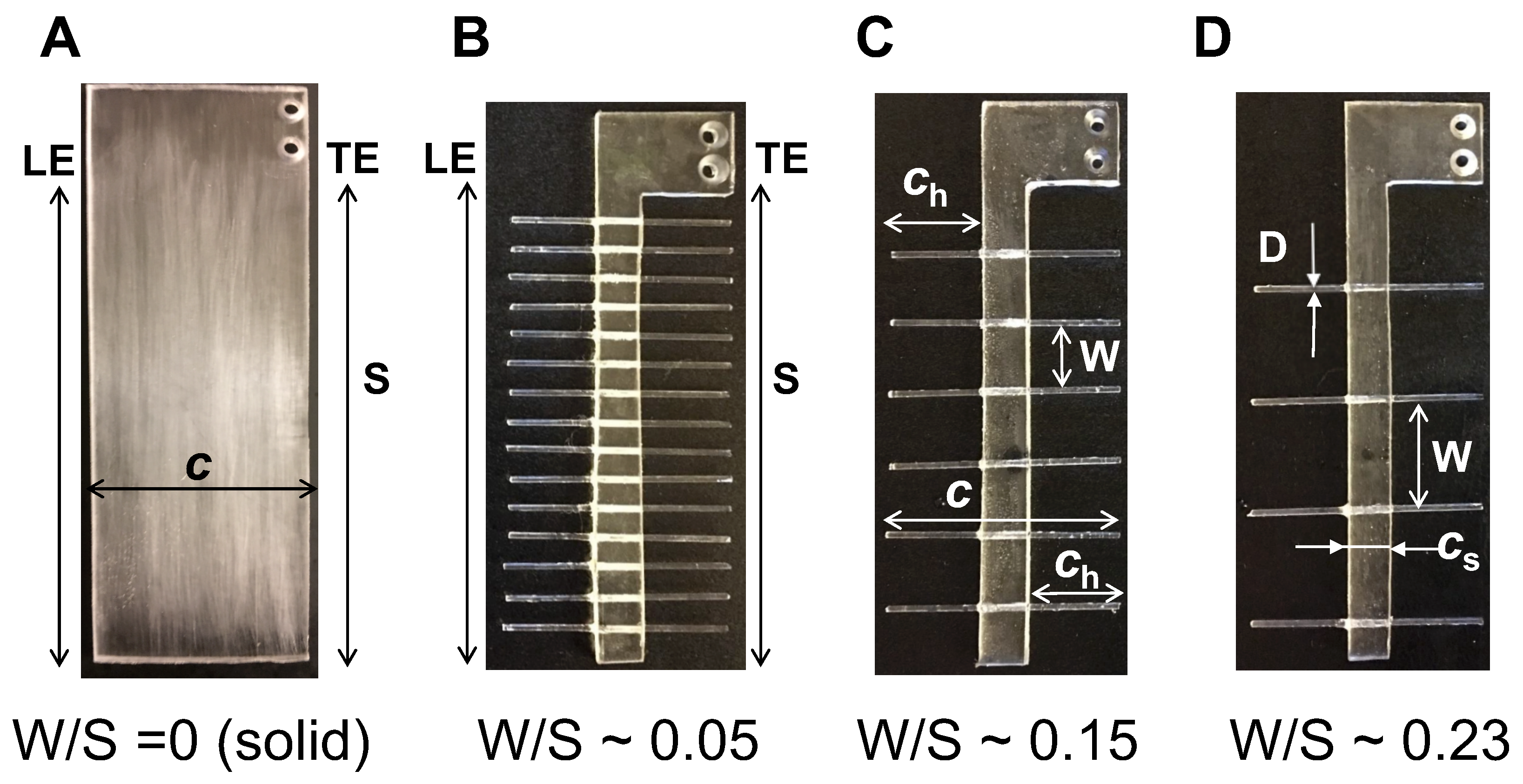
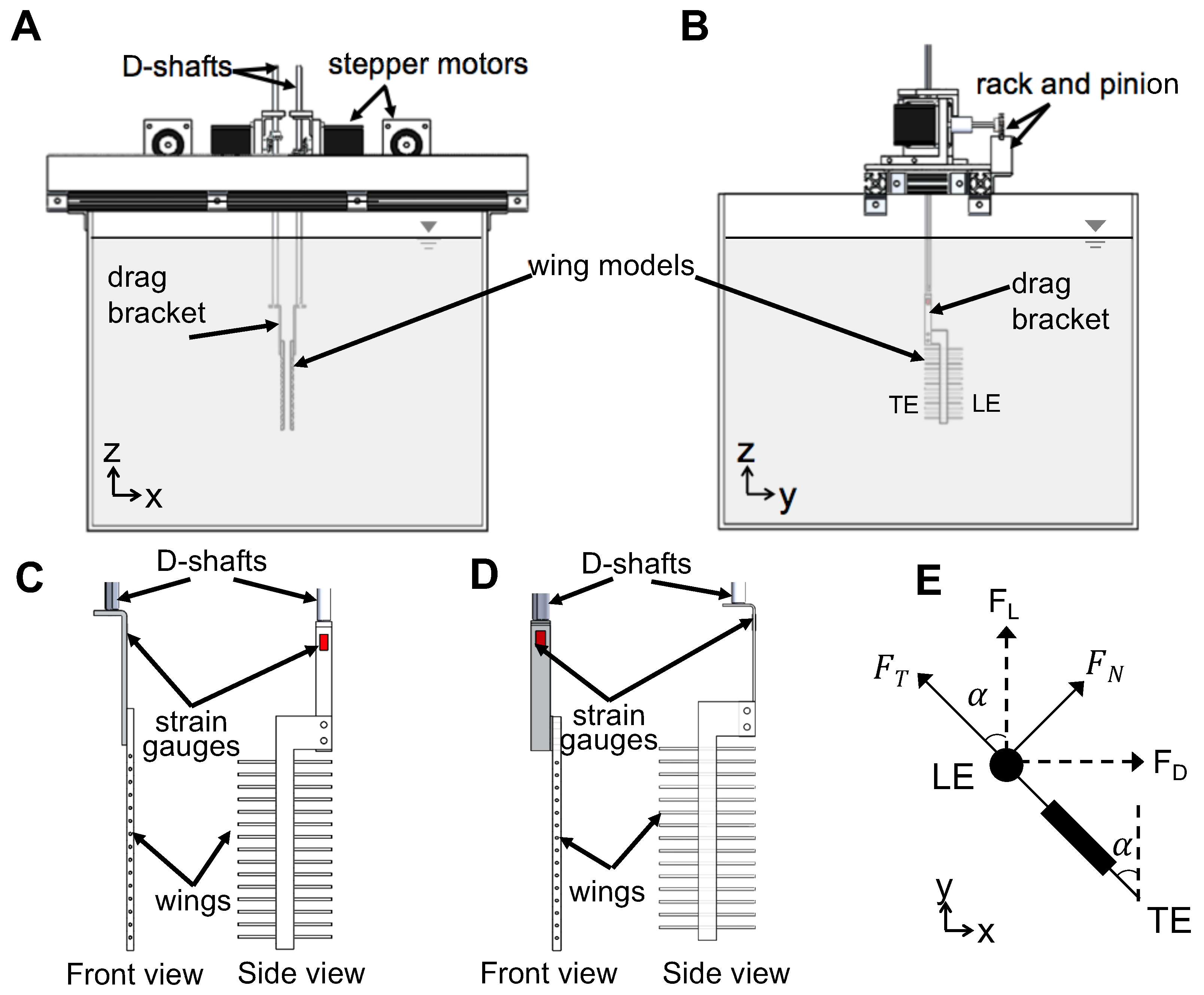
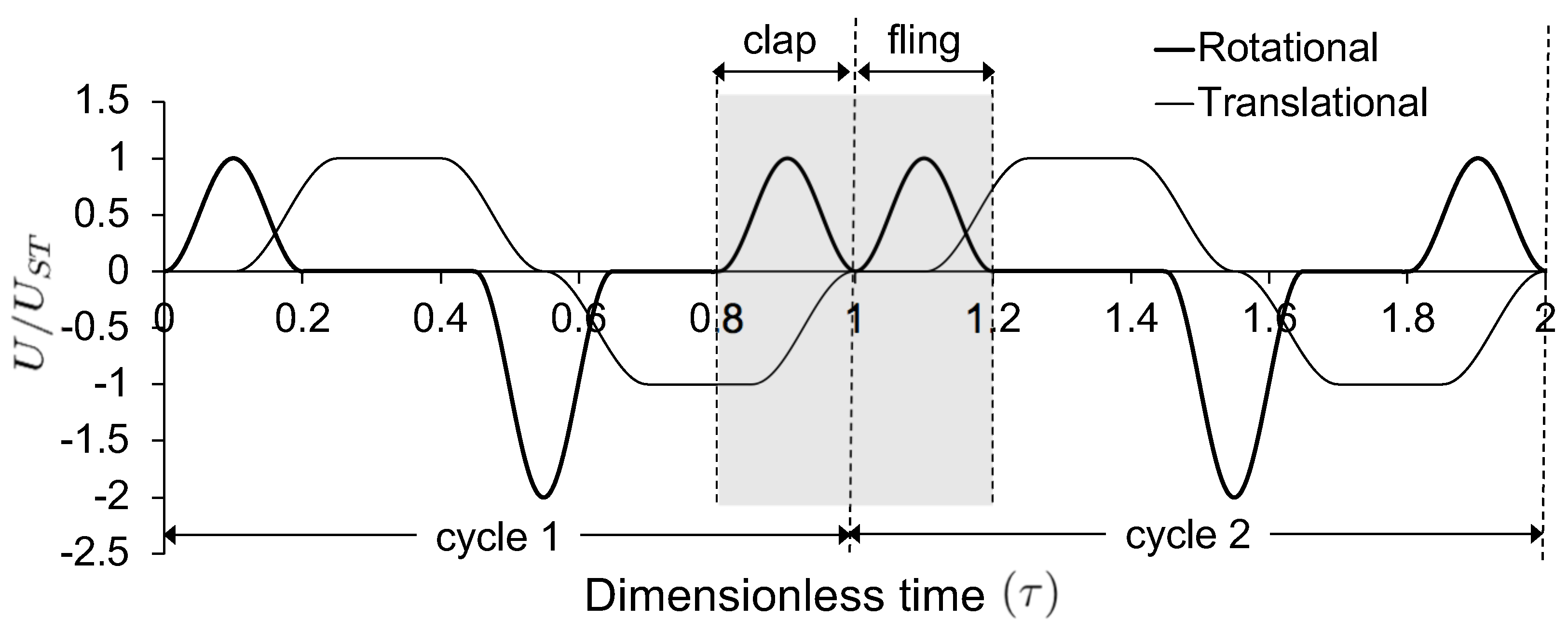
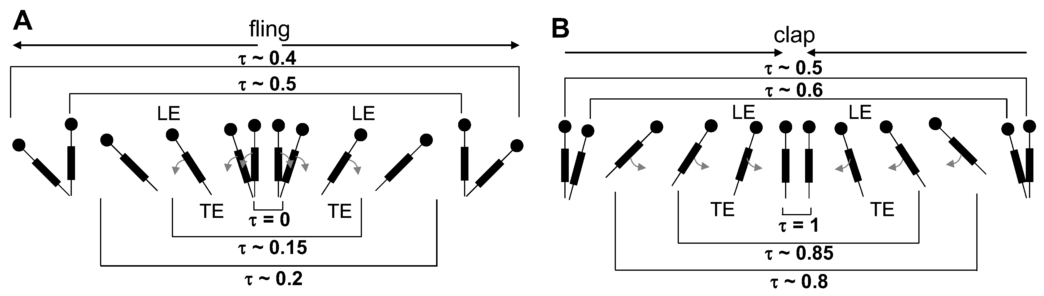
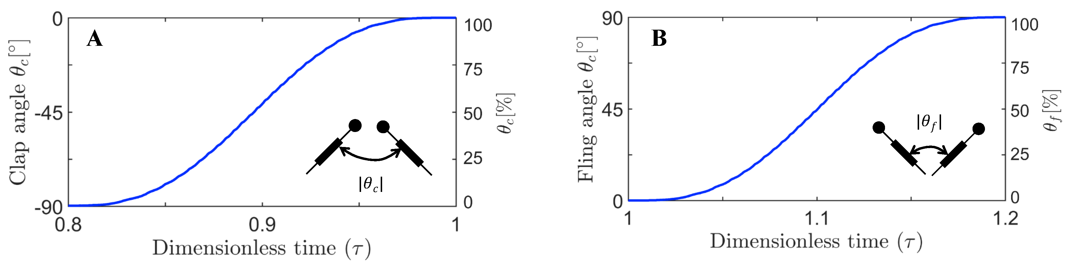
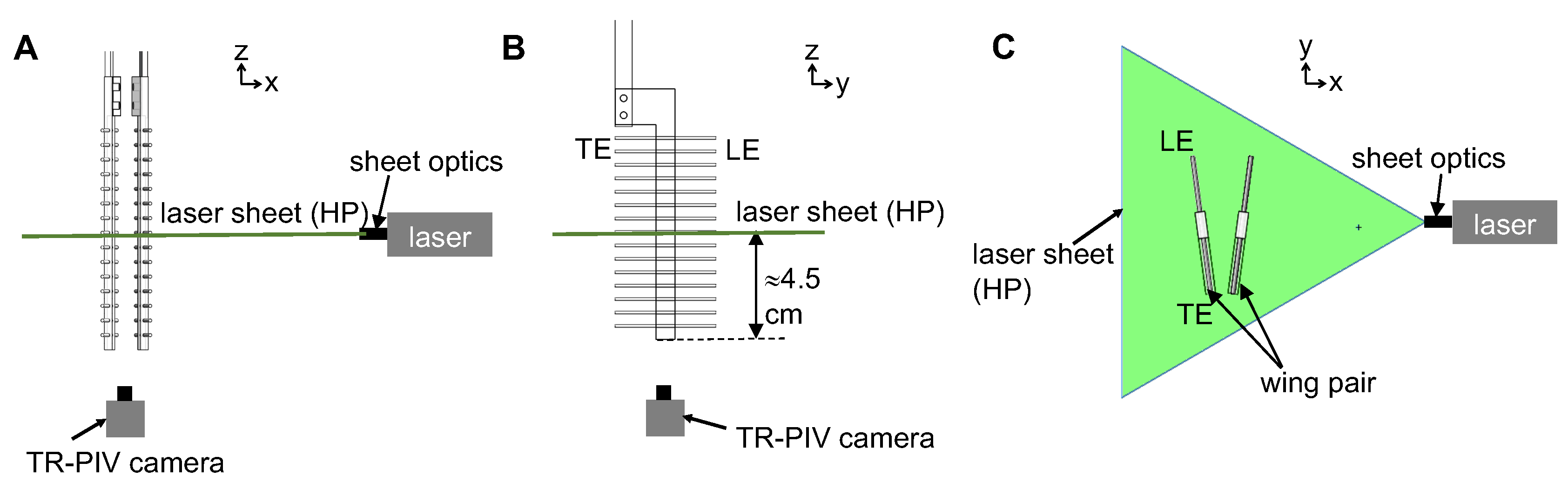
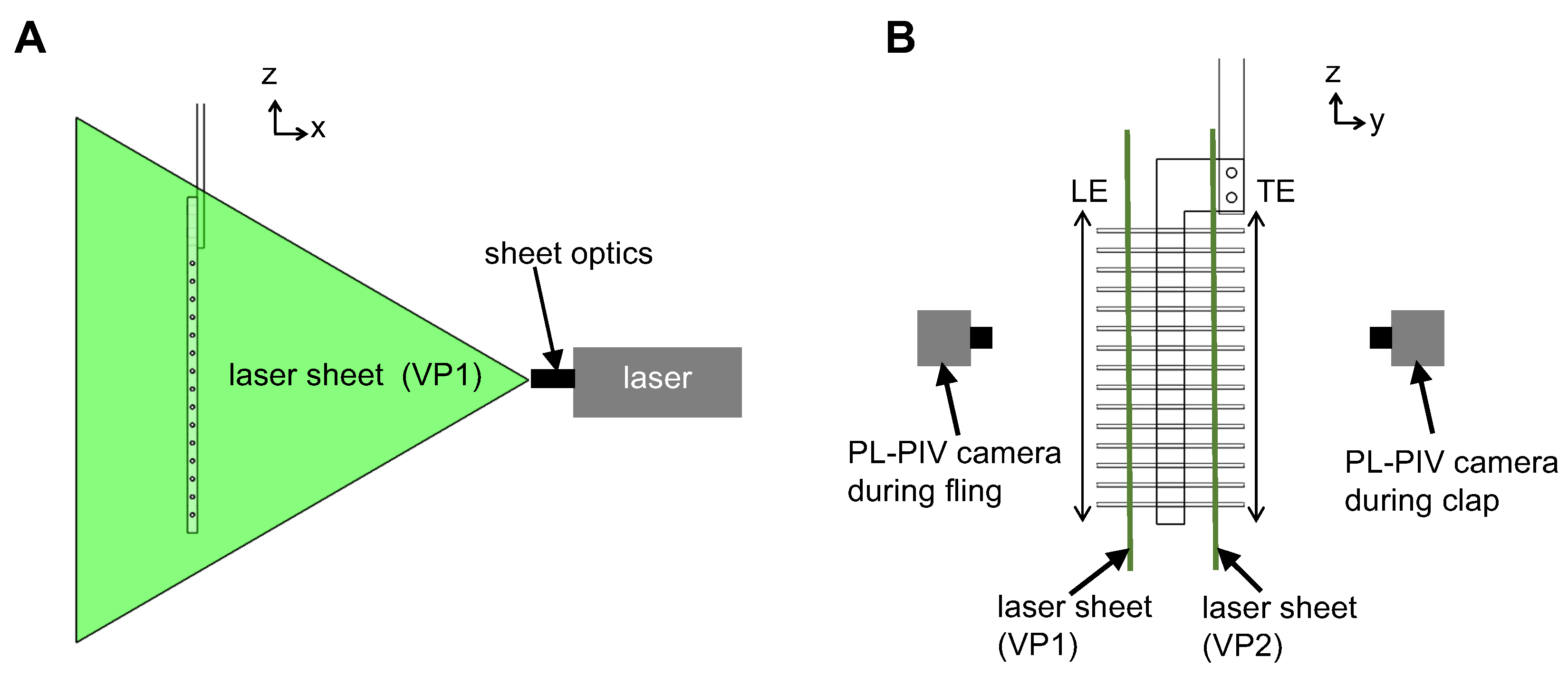
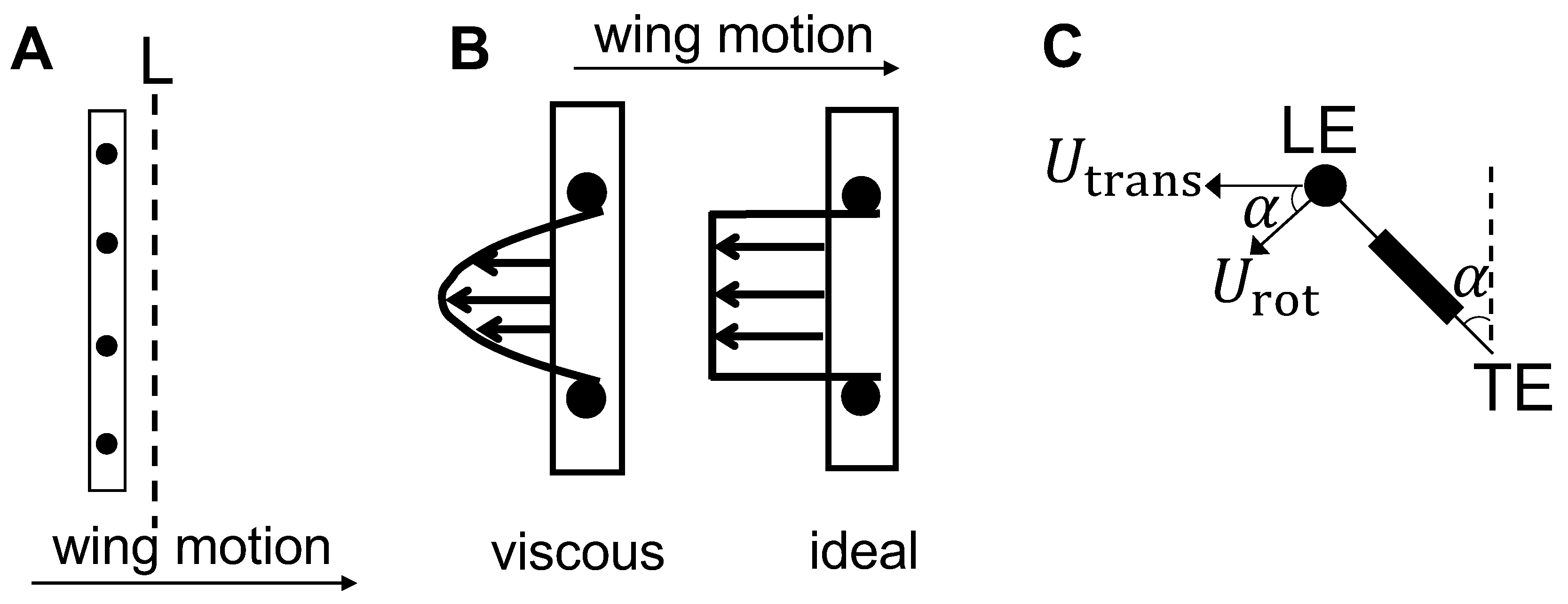
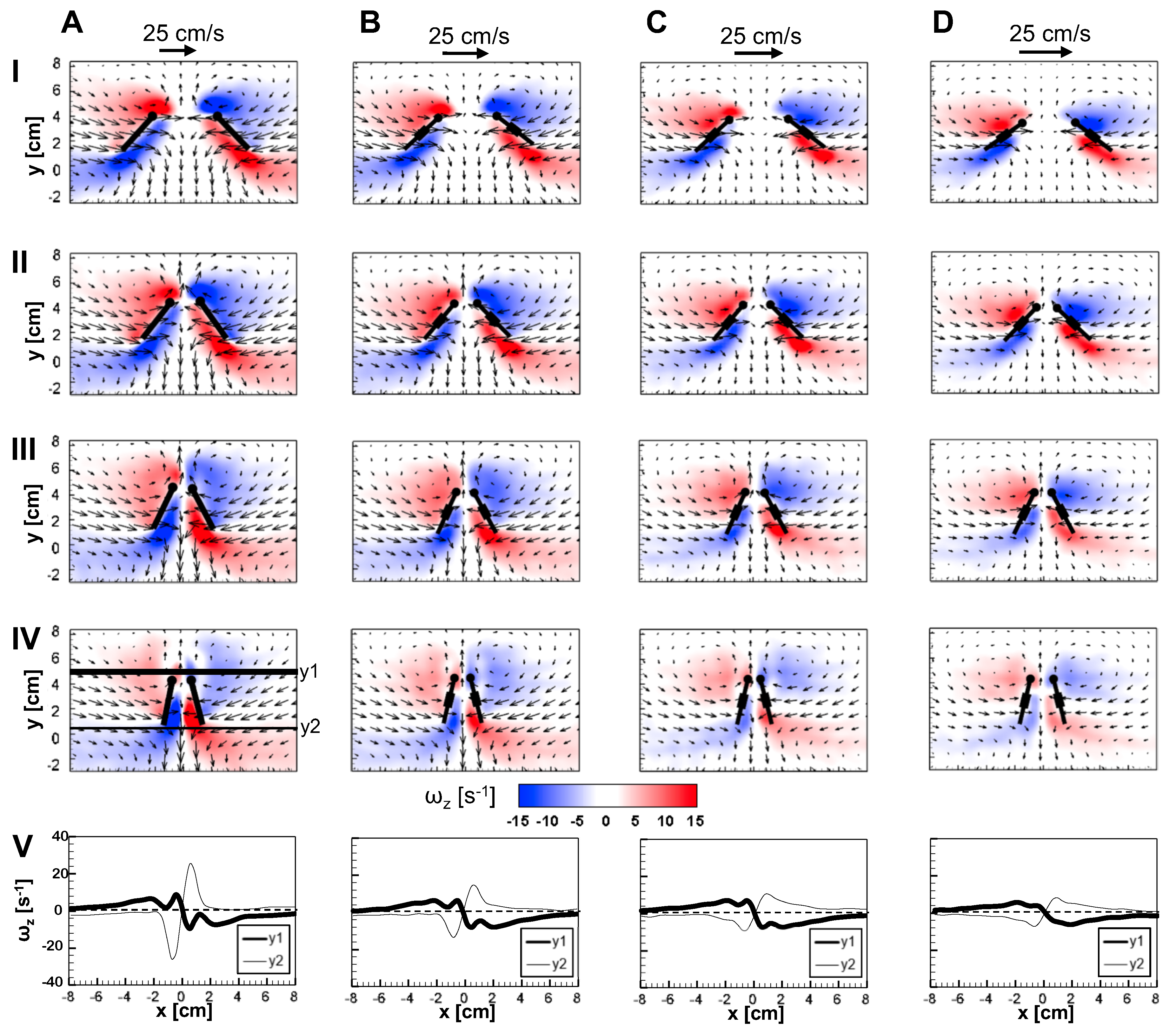
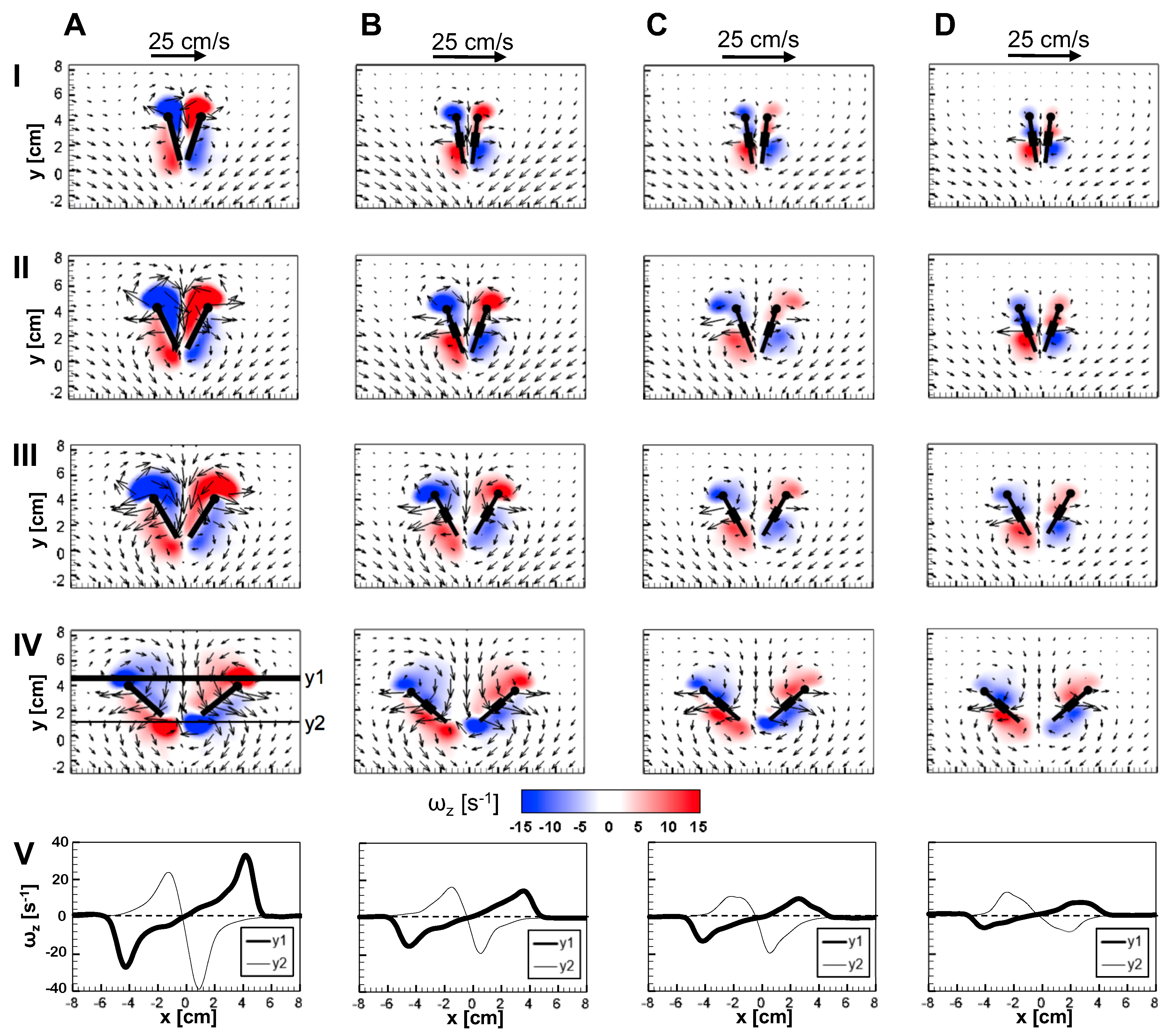
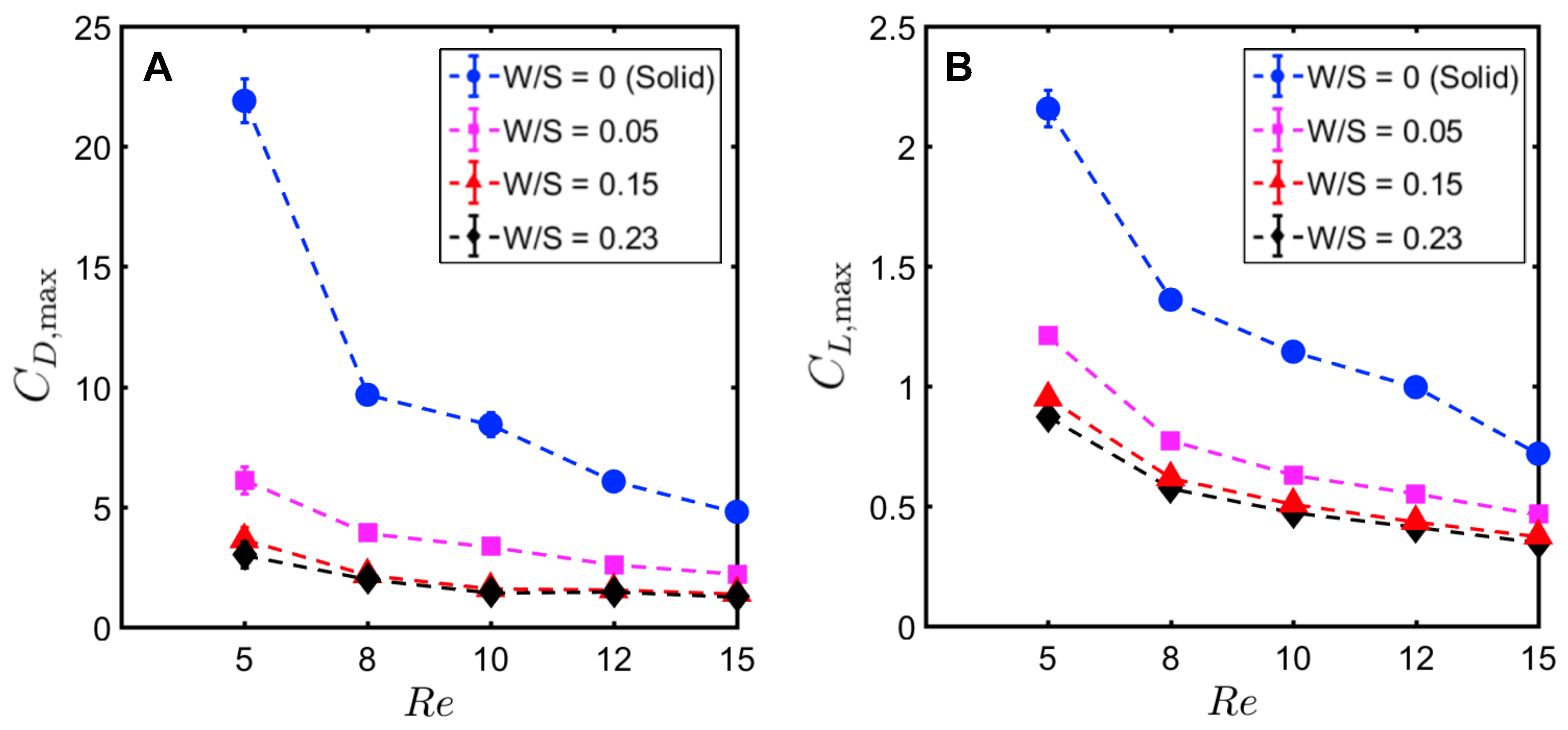
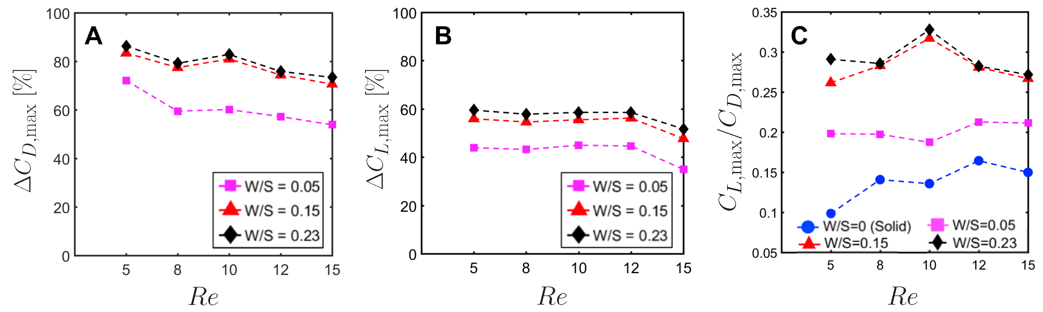
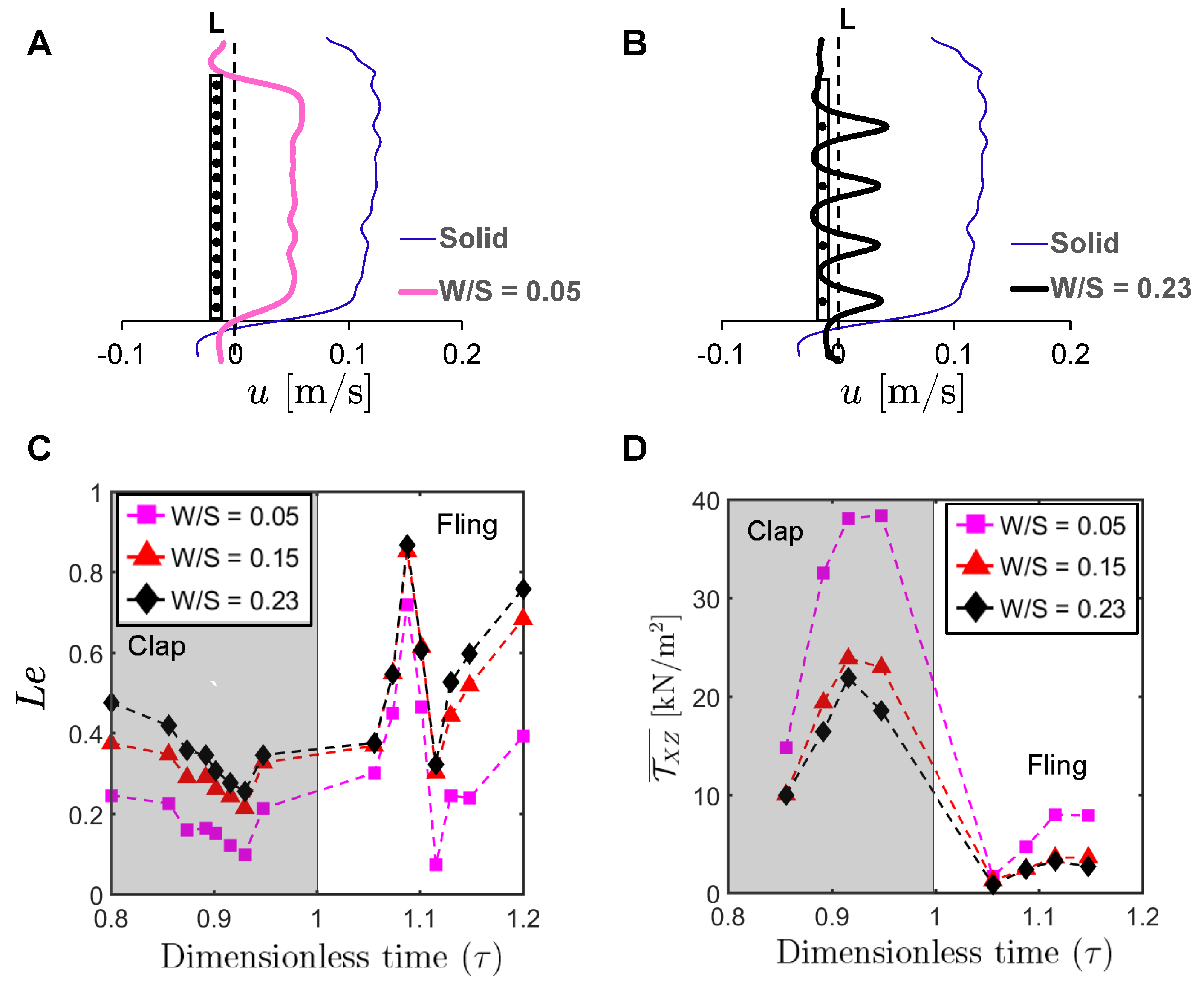
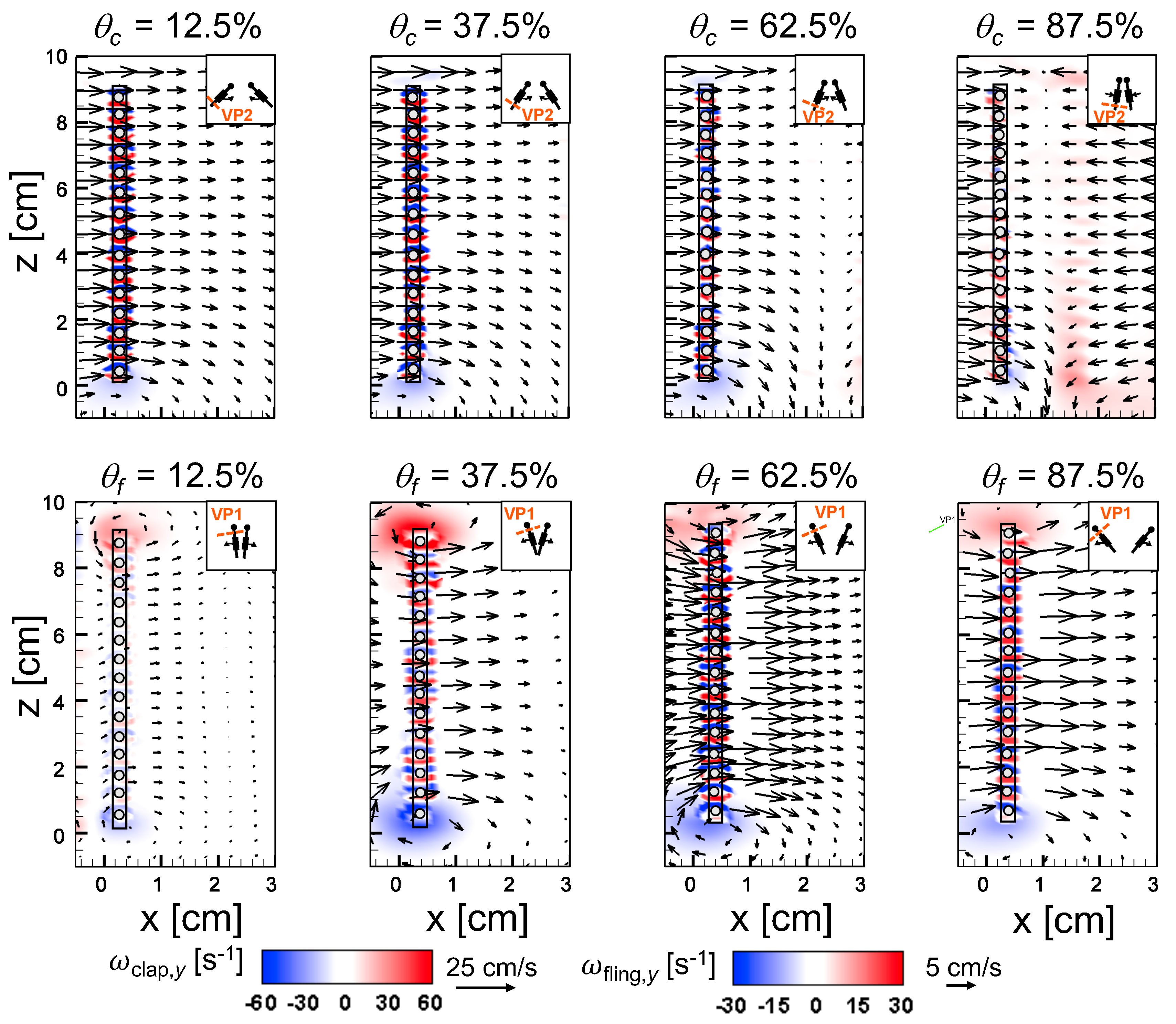
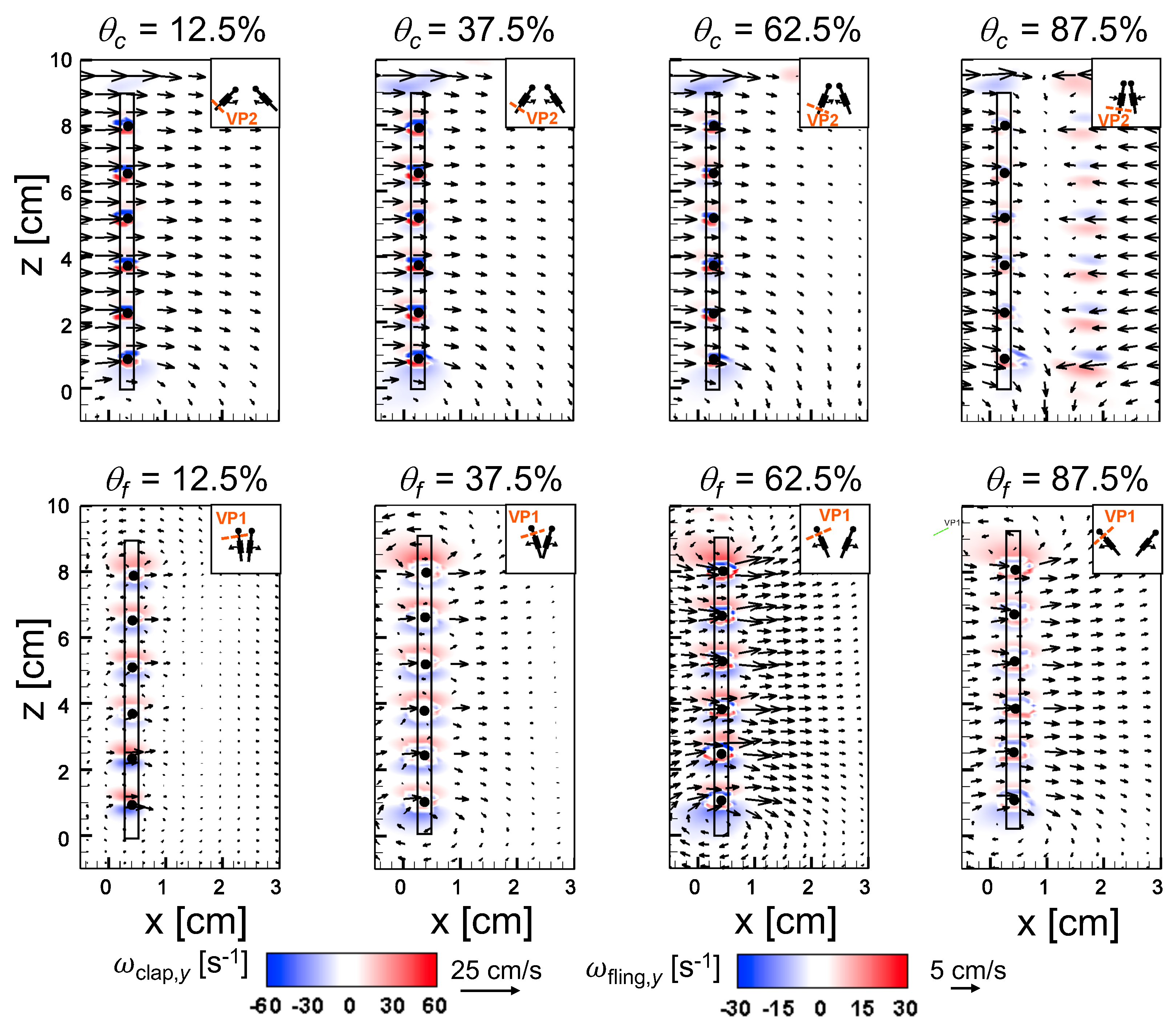
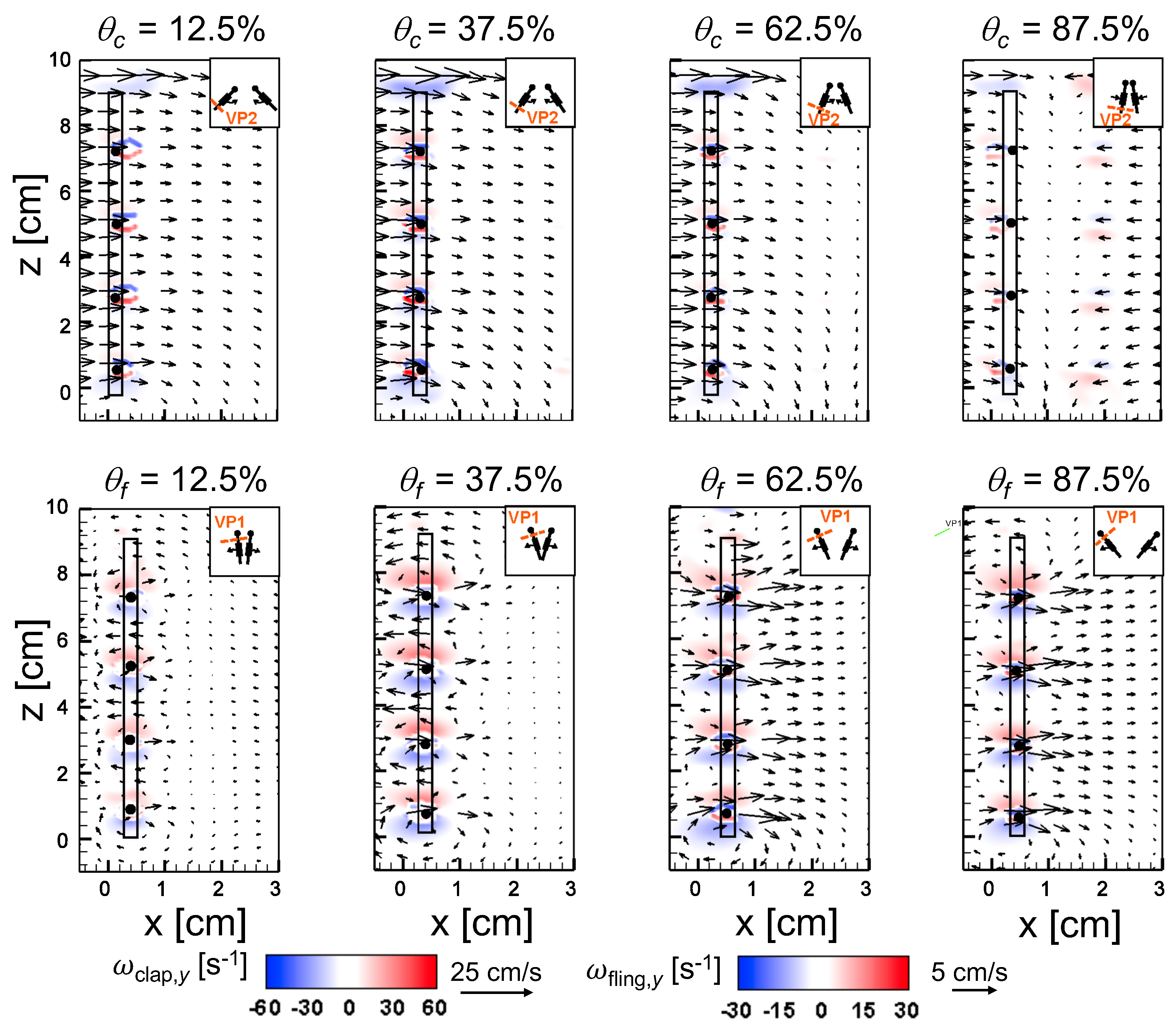
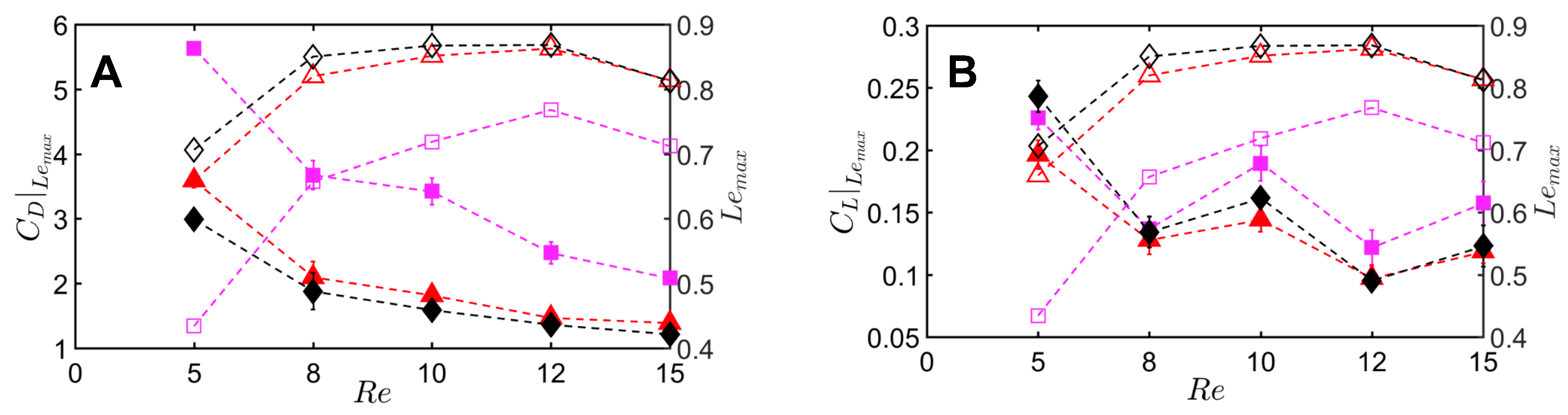
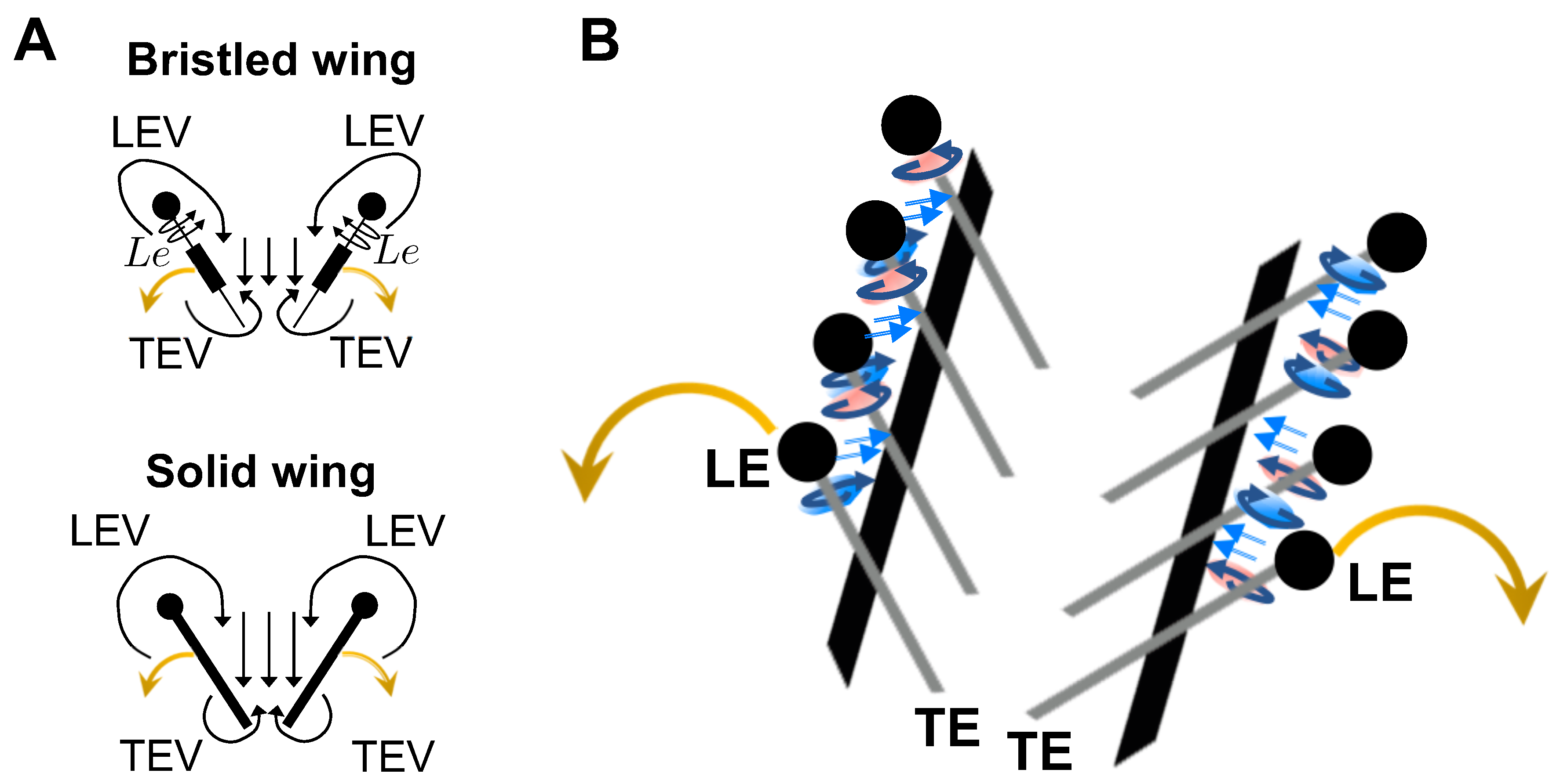
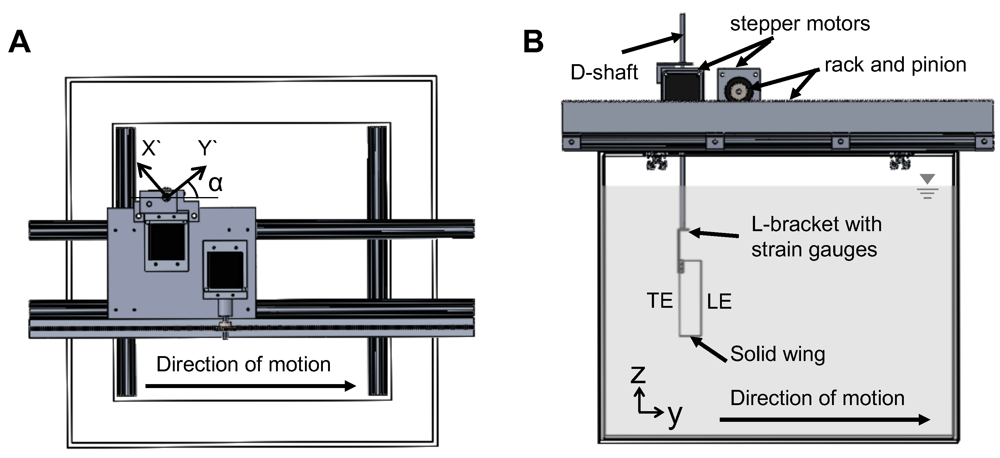
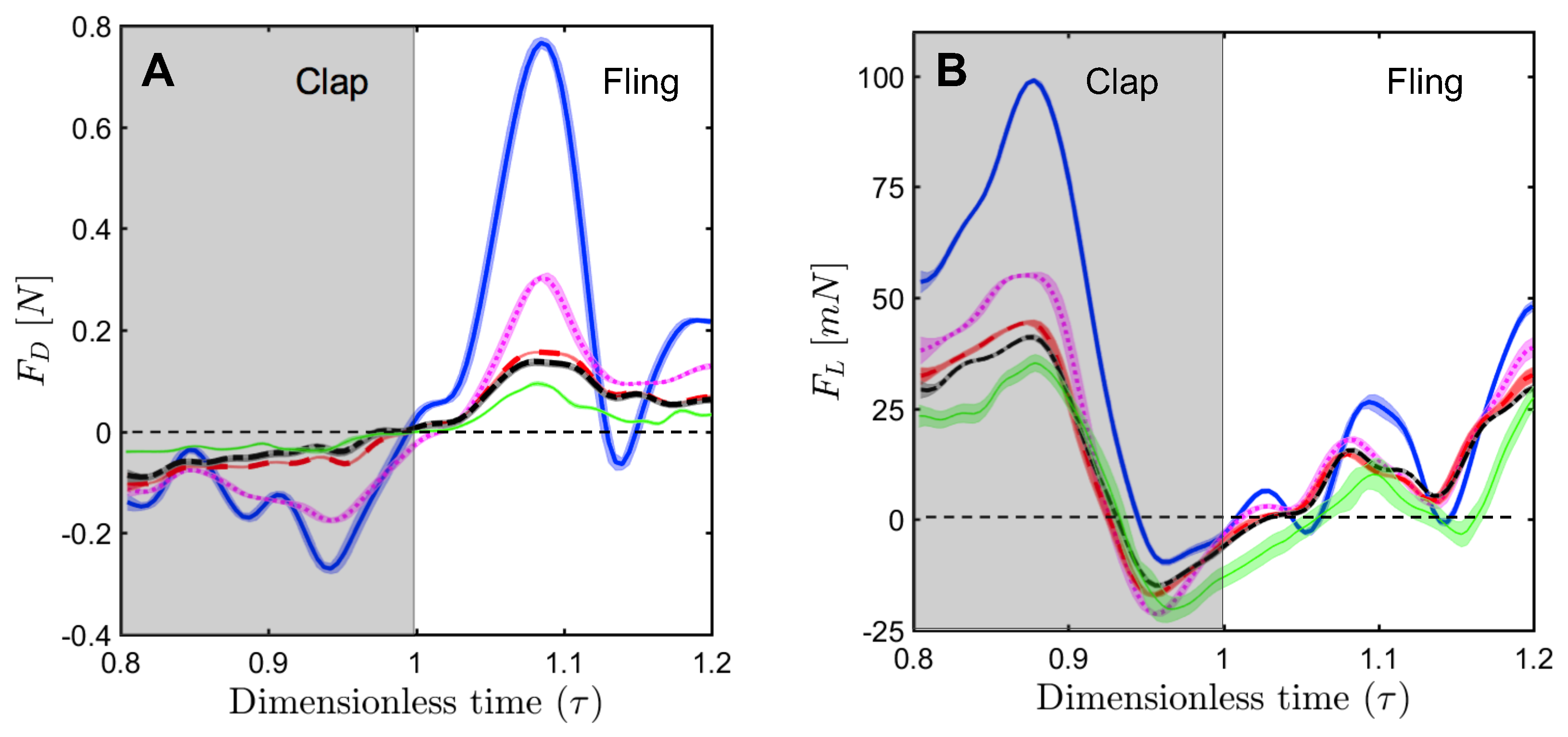
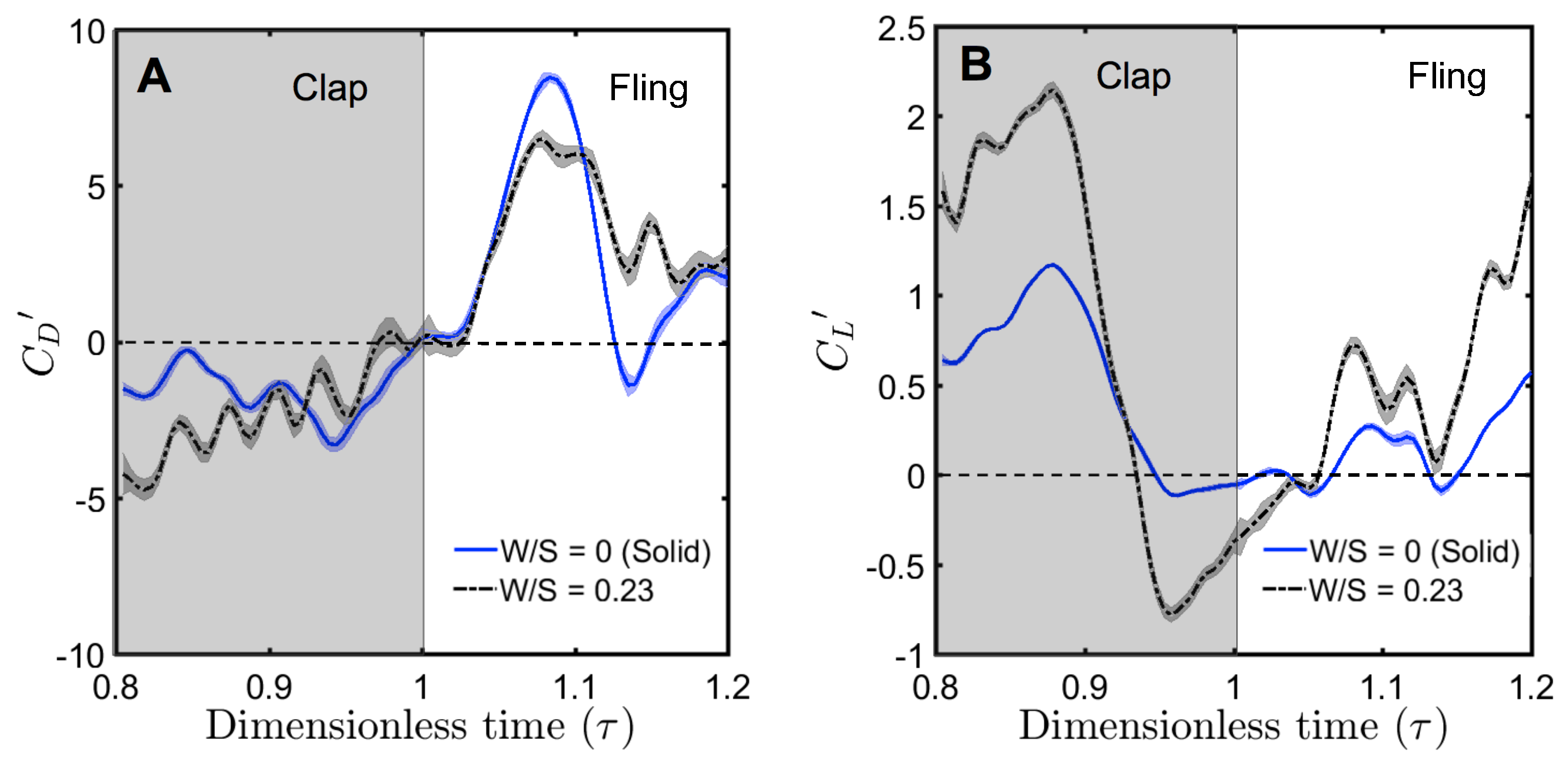
Table 1.
Experimental conditions used for PIV and force measurements comparing solid and bristled wing pairs during clap and fling. Camera recording rates used for time-resolved PIV (TR-PIV) measurements in chordwise plane () and phase-locked PIV (PL-PIV) measurements in spanwise plane () were varied to obtain data at identical non-dimensional time points () across every tested. Cut-off frequencies used for filtering strain gauge data () were varied for every . = steady translational velocity of the wing, = chord-based Reynolds number given by Equation (3), T = time taken to complete one cycle, which includes one fling half-stroke, stroke reversal, and one clap half-stroke (Figure 4).
| (cm/s) | Clap/Fling Duration (ms) | T (ms) | (frames/s) | (image pairs/s) | (Hz) | |
|---|---|---|---|---|---|---|
| 5 | 9.1 | 860 | 4300 | 116 | 0.12 | 12 |
| 8 | 14.6 | 540 | 2700 | 185 | 0.19 | 19 |
| 10 | 18.2 | 430 | 2150 | 233 | 0.23 | 23 |
| 12 | 21.9 | 360 | 1810 | 278 | 0.28 | 28 |
| 15 | 27.4 | 290 | 1450 | 345 | 0.35 | 35 |
© 2018 by the authors. Licensee MDPI, Basel, Switzerland. This article is an open access article distributed under the terms and conditions of the Creative Commons Attribution (CC BY) license (http://creativecommons.org/licenses/by/4.0/).
Share and Cite
MDPI and ACS Style
Kasoju, V.T.; Terrill, C.L.; Ford, M.P.; Santhanakrishnan, A. Leaky Flow through Simplified Physical Models of Bristled Wings of Tiny Insects during Clap and Fling. Fluids 2018, 3, 44. https://doi.org/10.3390/fluids3020044
AMA Style
Kasoju VT, Terrill CL, Ford MP, Santhanakrishnan A. Leaky Flow through Simplified Physical Models of Bristled Wings of Tiny Insects during Clap and Fling. Fluids. 2018; 3(2):44. https://doi.org/10.3390/fluids3020044
Chicago/Turabian StyleKasoju, Vishwa T., Christopher L. Terrill, Mitchell P. Ford, and Arvind Santhanakrishnan. 2018. "Leaky Flow through Simplified Physical Models of Bristled Wings of Tiny Insects during Clap and Fling" Fluids 3, no. 2: 44. https://doi.org/10.3390/fluids3020044