Quality Measures of Mixing in Turbulent Flow and Effects of Molecular Diffusivity

Abstract

Results from numerical simulations of the mixing of two puffs of scalars released in a turbulent flow channel are used to introduce a measure of mixing quality, and to investigate the effectiveness of turbulent mixing as a function of the location of the puff release and the molecular diffusivity of the puffs. The puffs are released from instantaneous line sources in the flow field with Schmidt numbers that range from 0.7 to 2400. The line sources are located at different distances from the channel wall, starting from the wall itself, the viscous wall layer, the logarithmic layer, and the channel center. The mixing effectiveness is quantified by following the trajectories of individual particles with a Lagrangian approach and carefully counting the number of particles from both puffs that arrive at different locations in the flow field as a function of time. A new measure, the mixing quality index Ø, is defined as the product of the normalized fraction of particles from the two puffs at a flow location. The mixing quality index can take values from 0, corresponding to no mixing, to 0.25, corresponding to full mixing. The mixing quality in the flow is found to depend on the Schmidt number of the puffs when the two puffs are released in the viscous wall region, while the Schmidt number is not important for the mixing of puffs released outside the logarithmic region.

1. Introduction

Turbulent flow is known to promote mixing in chemical reactors and other industrial processes. In fact, turbulent diffusion, which is one of the defining characteristics of turbulent flow [1], leads to enhancement in mixing [2]. A number of industrial applications depend on turbulent mixing [3,4,5,6,7], including combustion processes, and the design and operation of continuous stirred tank reactors (CSTRs) and plug flow reactors (PFRs), in addition to environmental processes that are important for weather changes and pollution dispersion [8,9]. While mixing because of molecular diffusion is a slow process [10], convective diffusion can significantly increase the mixing speed in turbulent flows. Yet, it has been noted that “the study of fluid mixing has very little scientific basis; processes and phenomena are analyzed on a case-by-case basis” (see J.M. Ottino’s introduction in [10]). In fact, several definitions of mixing have been proposed in the literature, while finding one that can fully describe mixing for industrial applications is still a matter of investigation [11]. Often, the measure of mixing is defined by examining the segregation between two substances, instead of the mixing [11,12].

A rather fundamental mixing process occurs when two clouds of different substances are released from point sources in a flow field. A cloud of particles or scalar markers resulting from an instantaneous release from a point or a line is called a puff (for example, consider a puff of smoke that comes out of the exhaust pipe of a car or a puff of smoke exhaled by a smoker), while a cloud of particles that results from a continuous release of particles is called a plume [13,14]. The behavior of a puff is the most elementary dispersion in a turbulent flow field, and can be used to investigate and understand quite fundamental mechanisms of turbulent dispersion [15,16,17], even though it is not easy to study experimentally, where the study of plumes is easier [18,19,20,21,22,23,24,25].

Using computations, it is feasible to simulate the dispersion of particles that mark the trajectory of scalar quantities (like heat or mass concentration) in turbulent flow. These computations are based on the Lagrangian framework, and they consist of tracking individual scalar markers in a flow field obtained through a computational fluid dynamics model. A lot of work has been done with turbulent dispersion in homogeneous, isotropic turbulence [26,27,28,29,30,31,32,33], as well as in anisotropic turbulent flow, like channel flow [34,35,36,37,38], where the flow field was obtained through a direct numerical simulation (DNS) or a large eddy simulation (LES) approach. Lagrangian methods offer the advantage of simulating dispersion cases with a range of molecular diffusivities and Schmidt numbers (Sc) that may span a wide range. Combining a DNS with Lagrangian scalar tracking (LST), our laboratory has produced results for simulations with Sc that covers several orders of magnitude (from Sc = 0.01 to Sc = 50,000) [17]. The main disadvantage of Lagrangian methods is the need to use a large number of scalar markers to simulate turbulent transfer and the slow convergence of particle-based methods [39]. Hybrid Eulerian-Lagrangian methods have been utilized recently [34], but the highest Sc achieved is in the order of Sc = 50. The use of DNS for the generation of the velocity field has the advantage of providing a high fidelity representation of the flow in which mixing occurs, but has the disadvantage that the Reynolds number (Re) for the flow field is relatively small [40,41,42,43], while LES or hybrid methods can get to higher Re values but with sacrifice in fidelity.

In the present work, a DNS/LST approach is employed to investigate mixing from instantaneous line sources of scalars released at different locations of a turbulent channel flow. Such an approach has been implemented to investigate the changes of the shape of a puff or scalar markers released in the middle of a turbulent flow channel [44] and to investigate mixing [45]. The contributions of this work are distinct from the contributions of prior work in that they (a) describe the concept of mixing quality with a quantitative measure; (b) investigate the characteristics of turbulent mixing in anisotropic turbulent flow; and (c) explore the effects of different Sc on mixing, with the use of results for Sc = 0.7, 6, 200, and 2400.

2. Materials and Methods

2.1. Flow Field Simulation and Lagrangian Scalar Tracking Approach

The velocity field is obtained using a DNS for a Newtonian and incompressible fluid in a fully developed Poiseuille channel flow. The turbulent flow is anisotropic, so that the velocity fluctuations and the turbulence statistics depend on the distance from the wall. The details of the DNS methodology have been published elsewhere [46] and have been validated with experimental measurements [44,47], while the LST approach [48] has also been validated with comparisons of the computational results to both experimental and Eulerian computational results [14,49,50]. The dimensions of the DNS computational box are 16πh × 2h × 2πh in the x (streamwise), y (wall-normal), and z (spanwise) directions, respectively, where the half-channel height (h) is 300. The driving force for the flow is a constant mean pressure gradient, and the resolution of the simulation is a grid with 1024 × 129 × 256 points in the x, y, and z directions, respectively. The spacing of the mesh is uniform in the streamwise and spanwise directions with periodic boundary conditions, while Chebyshev polynomial collocation points are used in the direction normal to the channel walls with no-slip and no-penetration boundary conditions on the rigid channel walls. The DNS algorithm is based on a pseudospectral fractional step method with the pressure correction suggested by Marcus [51,52]. The friction Reynolds number is Re_τ = h = 300, when the quantities are made dimensionless with the viscous wall parameters (i.e., the friction velocity, u*, and the kinematic viscosity of the fluid, ν). The friction velocity is given as u*= (τ_w/ρ)^1/2, where τ_w is the shear stress at the wall and ρ is the fluid density. Based on the mean centerline velocity and the channel half height, the Reynolds number is Re = 5760. The time step was 0.1 in viscous wall units, and the iterations were carried out for 30,000 time steps for stationary channel flow in order to simulate 3000 viscous time units of flow after the puffs are released.

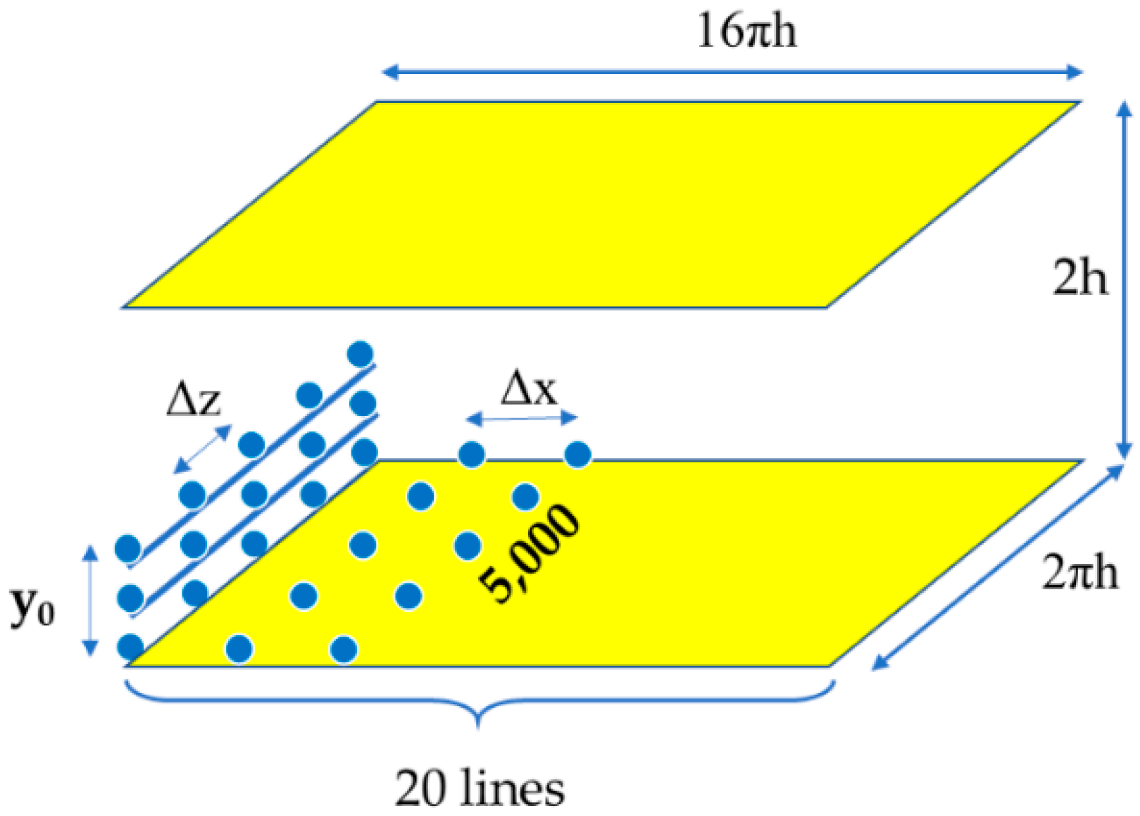
The trajectories of mass markers released from lines parallel to the z axis at different distances from the channel wall are calculated using the flow field created by the DNS. Data were generated for Sc covering four orders of magnitude (Sc = 0.7, 6, 200 and 2400) with markers released at a distance from the bottom channel wall equal to y_o = 0, 15, 75, and 300, as seen in Figure 1. This configuration allows the study of effects of turbulent convection and molecular diffusion on mixing at both small and relatively large times. The markers were released from 20 lines uniformly spaced along the x direction (at spaces of Δx = 16πh/20), with the first line starting at x = 0 for each distance from the wall. The released markers were also uniformly spaced in the z direction (spacing equal to Δz = 2πh/5000), so that 5000 markers were released on each one of the 20 lines. In this way, the total number of markers per distance from the wall, y_o, is 100,000 and the total number of markers per Sc is 400,000. Since the flow is homogeneous in the x and z directions, there is no statistically important difference in choosing the point of release, and by covering the x-y plane with particles released at each y_o, one can remove bias effects by velocity field peculiarities at the point of particle release. In order to obtain the statistics of the particle motion in the streamwise direction, the x coordinate of each particle was determined after subtracting the x coordinate at the marker point of release x_o, so that (x-x_o) was used as the streamwise marker location in the data analysis. The mass markers are passive, and they do not affect the flow field. The flow field used for the Lagrangian scalar tracking of the markers is the same for all Sc cases, so that the effects of the Sc can be observed rather than the effects of the flow. The mass markers were released after the flow field reached a stationary state [48]. The motion of the scalar markers was decomposed into a convection part and a molecular diffusion part. The convective part can be calculated from the fluid velocity at the particle position, so that the Lagrangian velocity at time t of a marker released at location $\overrightarrow{X_o}$ at time zero, is assumed to be the same as the Eulerian velocity at that particle’s location at the beginning of the convective step, i.e., $\overrightarrow{V}(\overrightarrow{X_{\mathrm{o}}},t)=\overrightarrow{U}[\overrightarrow{X}(\overrightarrow{X_o},t),t]$, where $\overrightarrow{V}$ is the Lagrangian velocity and $\overrightarrow{U}$ is the Eulerian velocity vector. The equation of particle motion is then:

$$\overrightarrow{V}(\overrightarrow{X_o},t)=\frac{\partial \overrightarrow{X}(\overrightarrow{X_o},t)}{\partial t}$$

(1)

The particle velocity is found by using a mixed Lagrangian-Chebyshev interpolation between the Eulerian velocity field values at the surrounding mesh points. The particle position integration in time is approximated with a second order Adams-Bashforth scheme. The above approach has also been used in [44,45]. The effect of molecular diffusion follows from Einstein’s theory for Brownian motion [53], in which the rate of molecular diffusion is related to the molecular diffusivity D as follows:

$$\frac{d\overline{X^2}}{dt}=2D$$

(2)

for diffusion in the x dimension. The diffusion effect is simulated by adding a random movement on the particle motion at the end of each convective step. This random motion is a random jump that takes values from a Gaussian distribution with zero mean and standard deviation σ, which is found using Equation (2) to be $\sigma = \sqrt{2∆t/Sc}$, where Δt is the time step of the simulation in viscous wall units, (Δt = 0.1). This approach has also been applied in [14,16,17,54].

2.2. Mixing Calculations

The mixing of scalar markers arriving at a location in the flow field was evaluated following the procedures detailed in [45]. Assuming that two puffs of particles (one of type A and one of type B) were released in the flow field, one needs to decide when they would be considered to be mixed. A length scale for mixing, r, can be defined as the maximum distance at which two mass markers can interact, so that when a particle A is close to a particle B at a distance smaller than r, the two particles are considered mixed. The length scale for mixing needs to be determined so that it is not too small (missing mixed particles) or too large (overestimating mixing) [12]. In this work, the mixing length scale was determined as the diameter of a sphere defined using the turbulent Schmidt number (Sc_t) and the Lagrangian time scale. The scale r is proportional to the length scale for particle turbulent diffusion, which is $\sigma = \sqrt{2\tau /S{c}_{\mathrm{t}}}$, in analogy to the standard deviation of the random molecular motion. This is the standard deviation of the distribution of particle motion for particles diffusing with a diffusivity related to the turbulent Schmidt number over a time scale τ that is defined based on a Lagrangian criterion. In analogy to the Lagrangian correlation coefficient for fluid particles, Saffman [55] defined a material correlation coefficient for the Lagrangian motion of scalar markers. The difference is that scalar markers can move off of fluid particles depending on their diffusivity. The integral of Saffman’s material correlation coefficient over time provides a material timescale for scalar turbulent motion, and this is the time scale used herein to determine the value of σ. This time scale has been determined in prior results from our lab to be [56]:

$$\tau =4.59+33.04{(\frac{y_{\mathrm{o}}}{h})}^{0.87} ({\mathrm{Sc}}_{\mathrm{t}} > 3)$$

(3a)

$$\tau =(0.98\ast S{c}_{\mathrm{t}}{}^{0.13})\left[4.59+33.04{(\frac{y_{\mathrm{o}}}{h})}^{0.87}\right] ({\mathrm{Sc}}_{\mathrm{t}} \le 3)$$

(3b)

while the average Sc_t in the flow channel has been found to be Sc_t = 1.0257 (based on averaging the data in Figure 6 of ref. [35], where the Sc_t has been calculated as a function of distance from the channel wall). Since there is 95% probability for a Gaussian random variable to be within 2σ of its mean, we can assume that 95% of the motion of a scalar particle within time τ is going to be within a sphere of diameter 4σ, with σ determined as above. The average value of τ is 21.76, so that σ = 6.5 in viscous wall units. A circle with the diameter 4σ has an area of 533 square wall units. Therefore, the whole channel is divided into square bins of size 20 × 20 in the x and y directions, respectively, so that the bin area is in the same order of magnitude as the area of the particle motion when projected on the x-y plane (i.e., 400 square wall units is close to 533 square wall units). Bins of this size account for the mixing length scale used herein.

The total number of bins in the x and y directions were:

$$N_{binX}^{}=\frac{4\ast L_X}{∆bi{n}_X}; N_{binY}^{}=\frac{2h}{∆bi{n}_Y}$$

(4)

where the bin size is $∆bi{n}_X=∆bi{n}_Y=20$, L_X is the computational box length in the x direction, and 2h is the channel height. Each bin in the system can be denoted as bin (i,j), with 1 ≤ i ≤ $N_{binX}^{}$ and 1 ≤ j ≤ $N_{binY}^{}$. In the flow direction, there were enough bins to cover four times the channel length (this can be accomplished by taking advantage of periodicity in the streamwise direction and by allowing a particle that exits the box from one side to enter the box from the other side). This length was sufficient to track all the particles within 3000 viscous wall time units. Tests with bins starting at different positions showed negligible difference in the results regarding mixing [45].

3. Results

3.1. Development of Mixing Region with Time

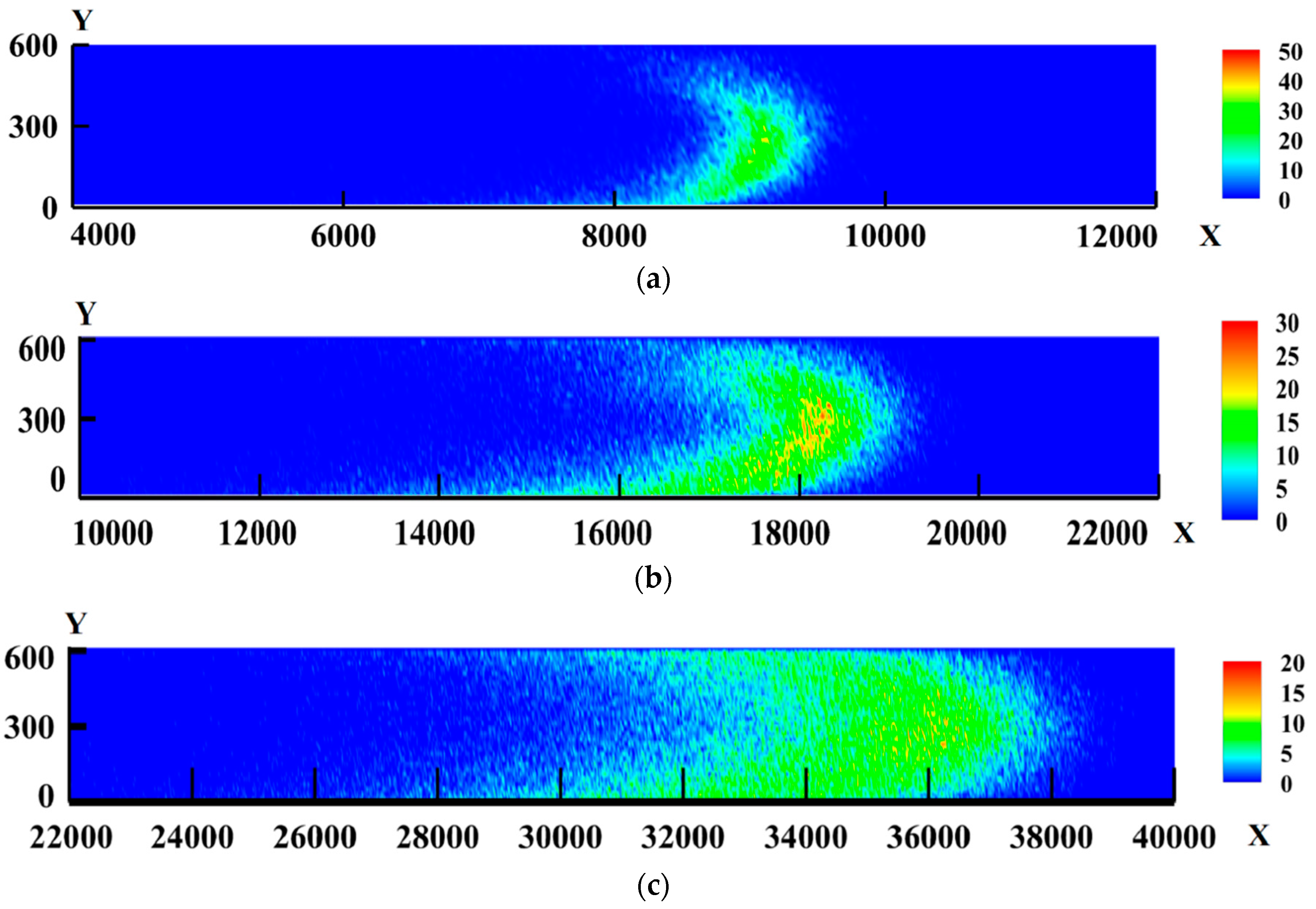
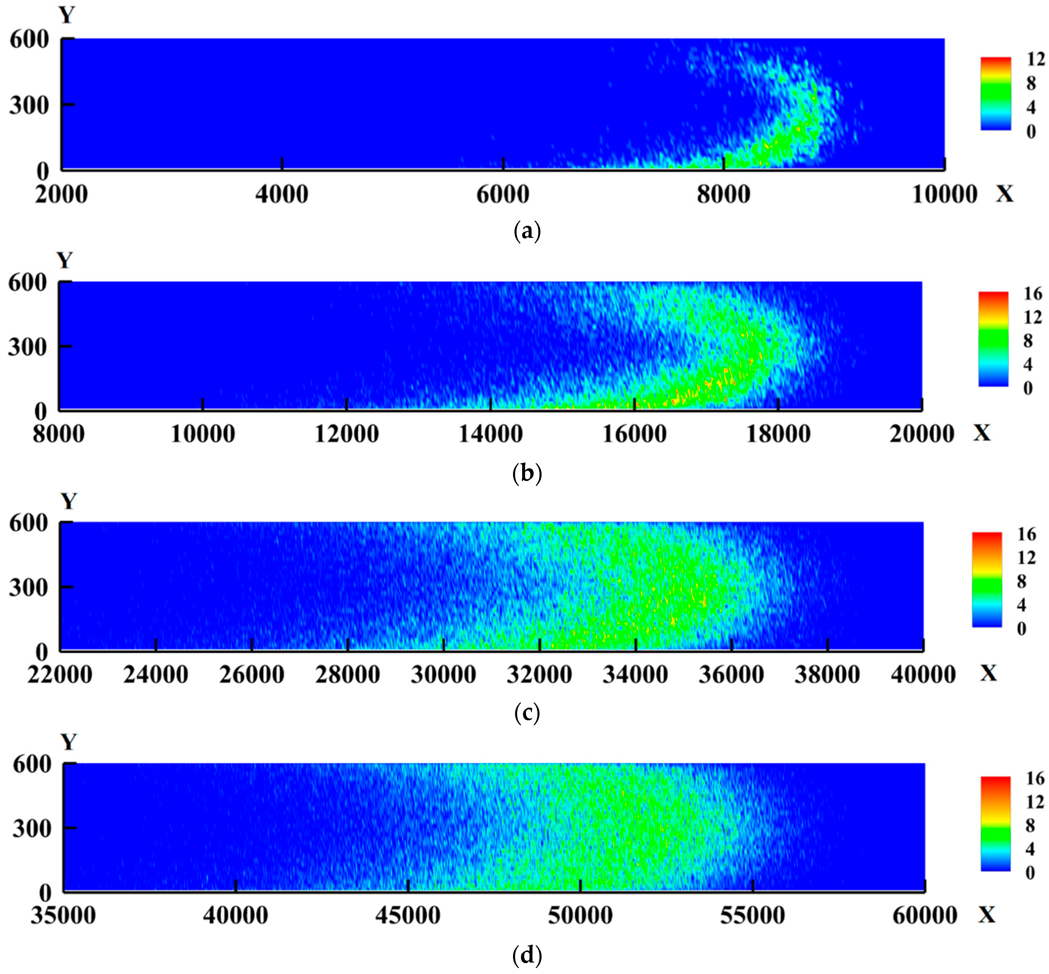
Figure 2a–d are contour plots of the development of the mixing region from puffs released at the center line of the channel and at y = 75 as a function or time t after their release. In this case, particles of type A are particles with Sc = 0.7 released from the center of the channel (at y_o = 300). This puff is designated as 0.7y300. Particles of type B are particles of the same Sc (Sc = 0.7), but released at y_o = 75, designated as 0.7y75. This notation will be adopted herein to denote the Sc of a puff and the location of its release. The contour colors in Figure 2 denote the number of mixed particles in each location, defined as the minimum particle count of particles of type A or B found in a bin. The idea is that if there are n_A(i,j) particles of type A in bin (i,j), and n_B(i,j) particles of type B in the same bin, then the mixing will be characterized by the minimum of n_A(i,j) and n_B(i,j). When this number is high, it means that the intensity of mixing is high. Figure 2 is a presentation of the quantity n_AB(i,j) = min[n_A(i,j), n_B(i,j)], and in this respect, it represents the development in time of the shape of the mixing zone and of the mixing intensity in the flow field.

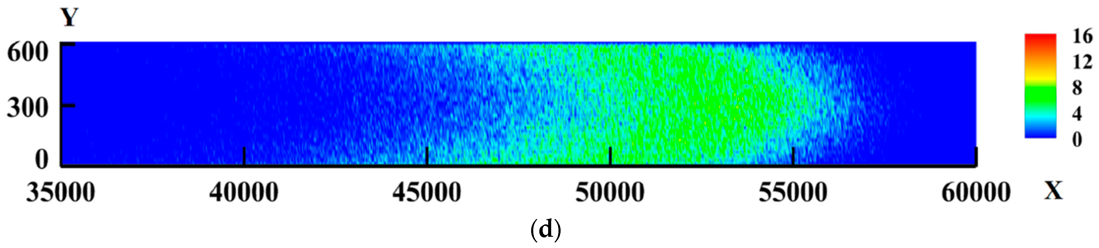
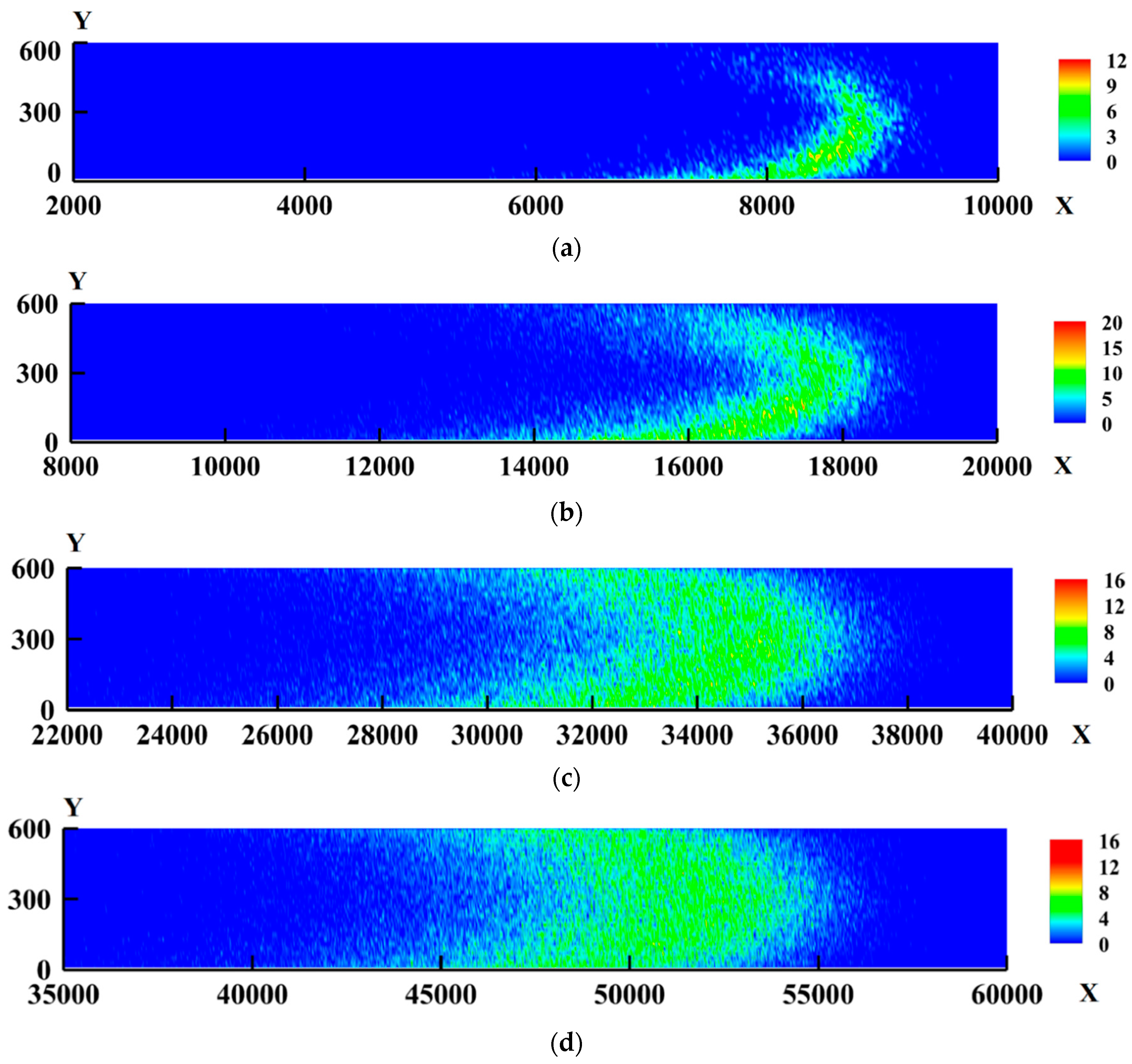
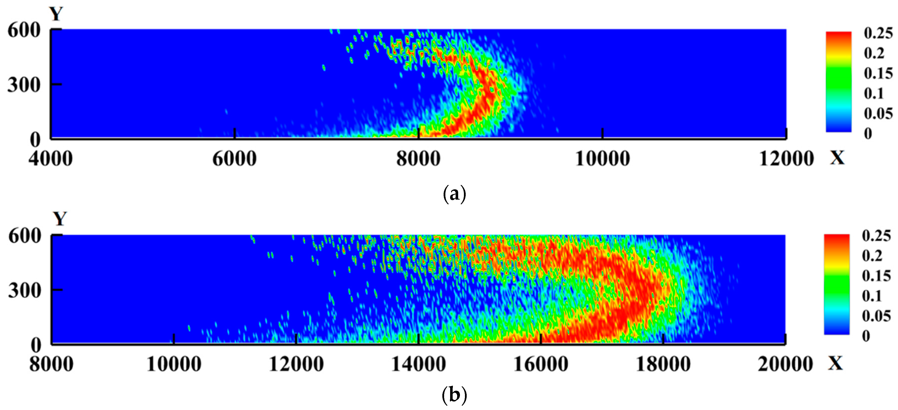
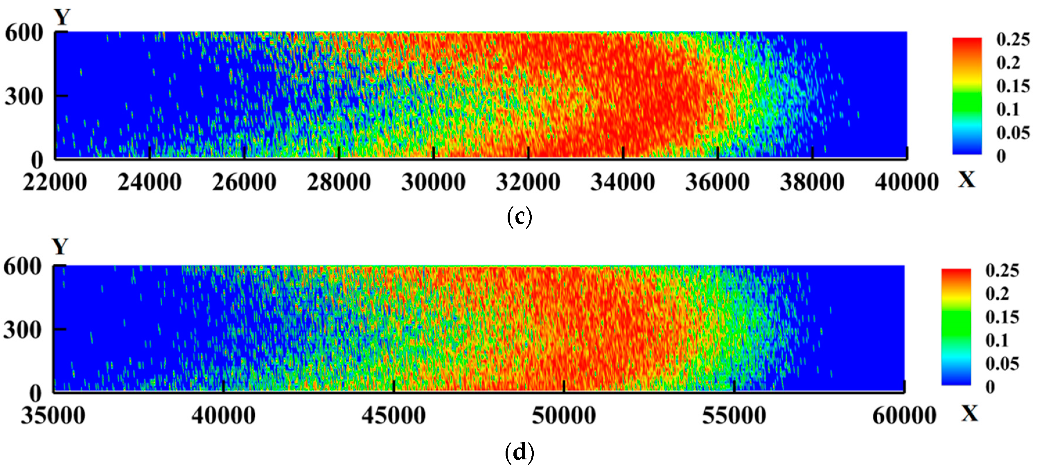
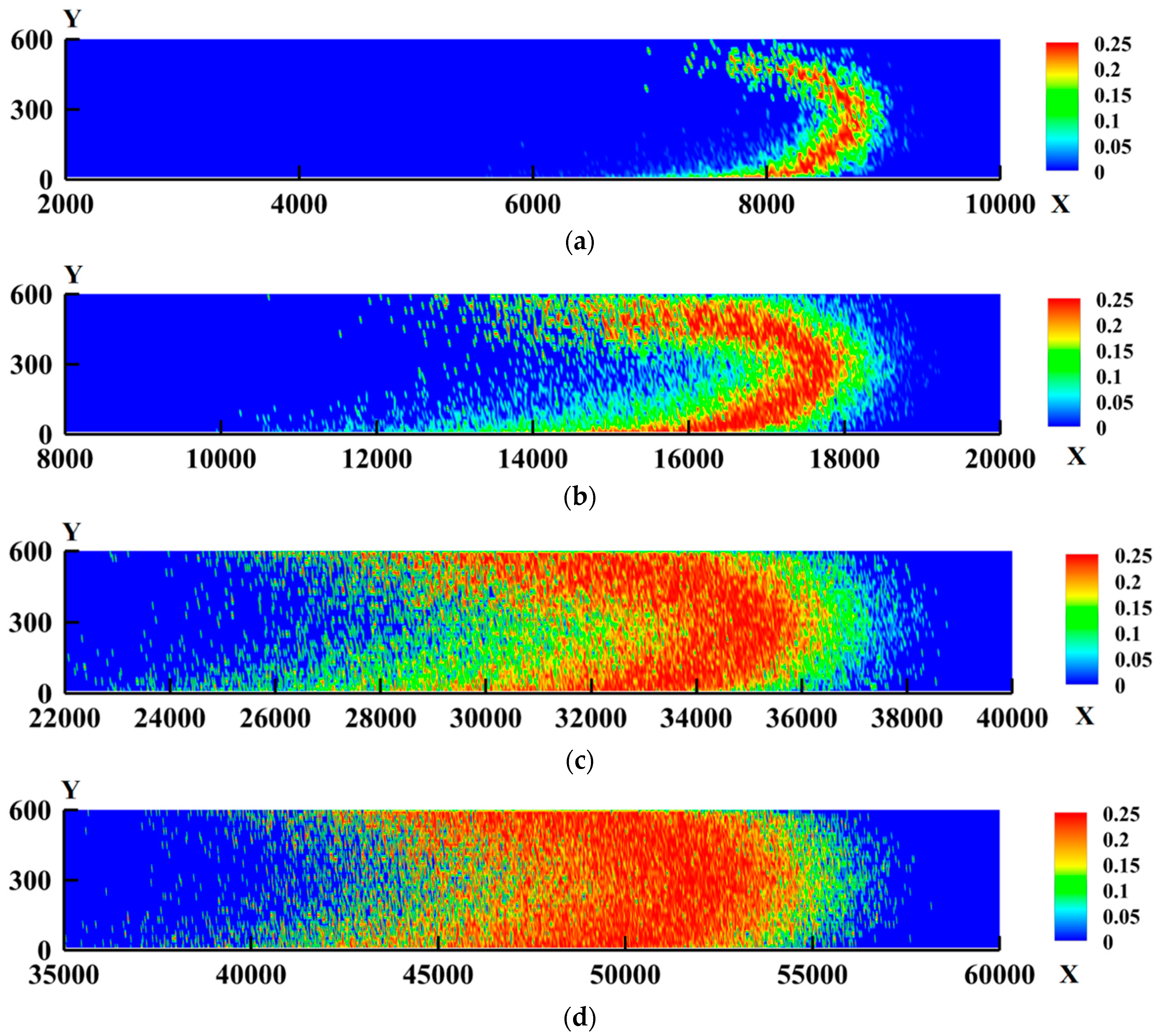
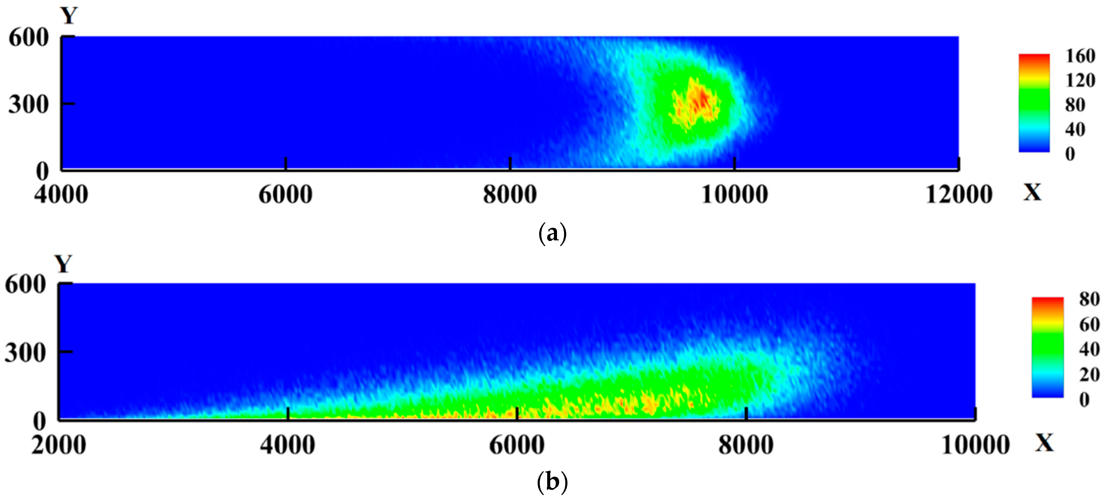
Figure 3a–d are plots of the mixing region for puffs 0.7y300 and 0.7y15. The Sc is the same for these two puffs, but the location of release of the second puff is at y_o = 15, so that differences in the development of mixing can be seen when compared with the case shown in Figure 1. Since past work has indicated that the Sc of the puff released in the center of the channel is not important for mixing, only figures for puffs with Sc = 0.7 released from the channel center are shown. However, the Sc of the puff released closer to the wall is important for the development of the mixing zone. This is why in Figure 4a–d, plots of the mixing region for puffs 0.7y300 and 2400y15 are presented.

3.2. Quality of Mixing

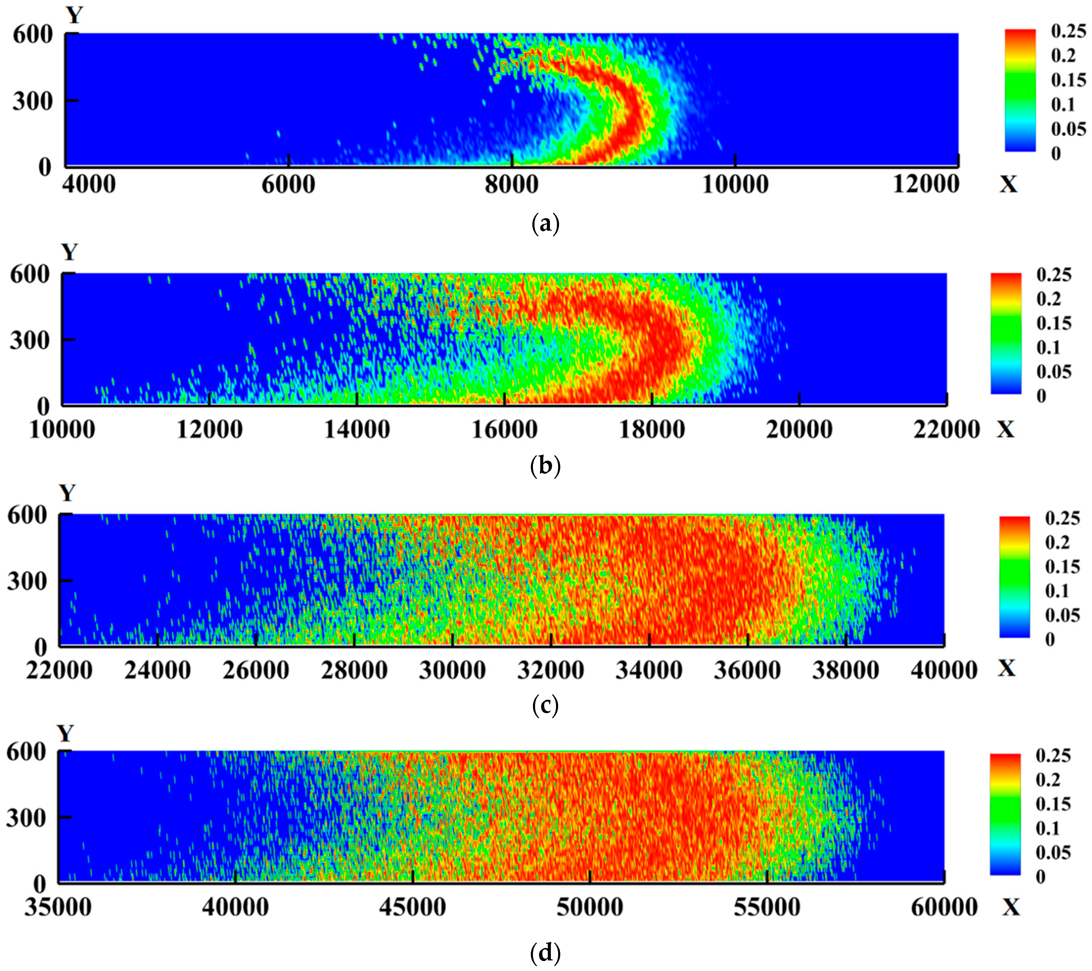
Figure 2, Figure 3 and Figure 4 are depictions of the mixing intensity, as expressed by n_AB, but there is a chance that particles are mixed, but not efficiently. This means that there might be many particles of one type in a bin, but there might be multiples of this number of particles of the other type in the same bin. To make this point clearer, when the number of particles of each type in a bin is the same, i.e., n_A(i,j) = n_B(i,j), then the quality of mixing is considered to be best, as opposed to a case where n_A(i,j) = C n_B(i,j), with C being a large coefficient. In order to quantify the quality of mixing in a location in the flow field, a new measure is introduced in this study, the mixing quality index, ϕ, defined as the product of the particle fraction in each bin (i,j), as follows:

$$\phi (i,j)=\frac{n_A(i,j)\times n_B(i,j)}{{\left[n_A(i,j)+n_B(i,j)\right]}^2}$$

(5)

The above quantity has the advantage that it is monotonically increasing with the quality of mixing. When only particles from puff A or from puff B are present in a bin, the value of ϕ(i,j) is zero. The maximum value of ϕ occurs when half of the particles in a bin are from puff A and half from puff B—at that point the value of the mixing quality index is ϕ_max = 0.25. Figure 5, Figure 6 and Figure 7 are plots of the development of the mixing quality index for puffs 0.7y300 and 0.7y75, puffs 0.7y300 and 0.7y15, and 0.7y300 and 2400y15.

One can also define an overall mixing efficiency that can combine the intensity of mixing with the quality of mixing across the channel in the following manner:

$$m=\frac{{{\displaystyle \sum }}_{i=1}^{N_{binX}}{{\displaystyle \sum }}_{j=1}^{N_{binY}}{n}_{AB}(i,j) \phi (i,j)}{N_t {\phi }_{max}}$$

(6)

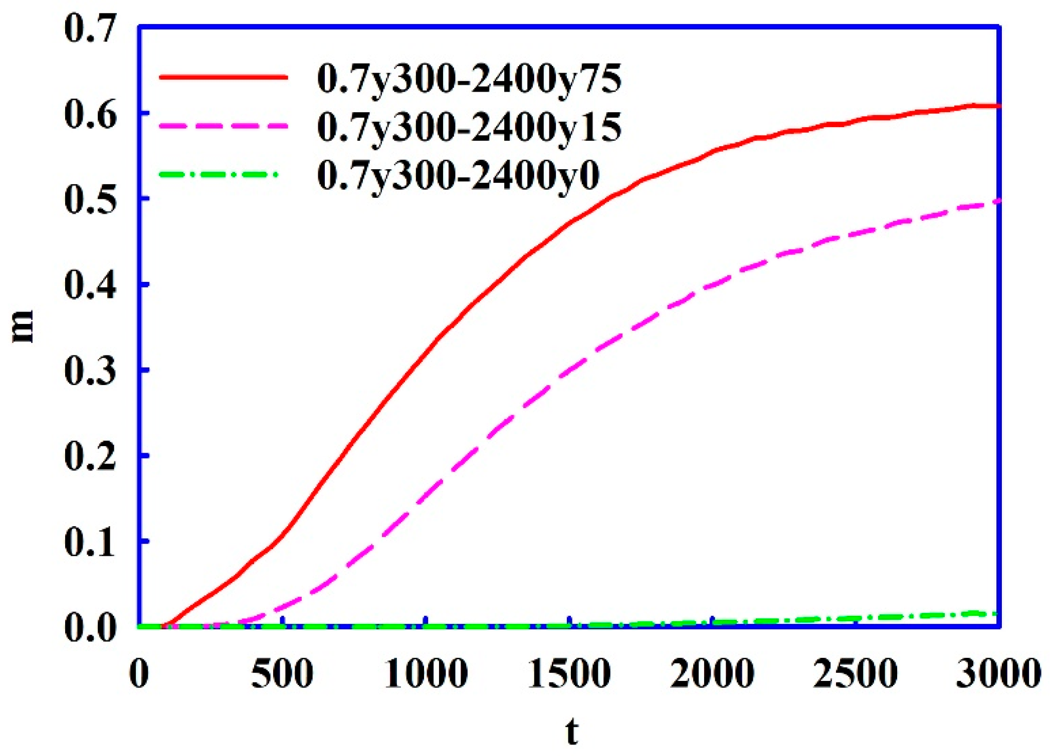
The measure m can take values between zero and one (N_t is the total number of particles released in each puff, in this case, N_t = 100,000). When it approaches zero, there is either no mixing or the quality of mixing is very poor, and when it approaches one, the particles are half of type A and half of type B in each bin. Figure 8 is a plot of the change of m with time for the cases of puff A being released from the center of the channel (0.7y300) and puff B released at different distances from the wall of the channel.

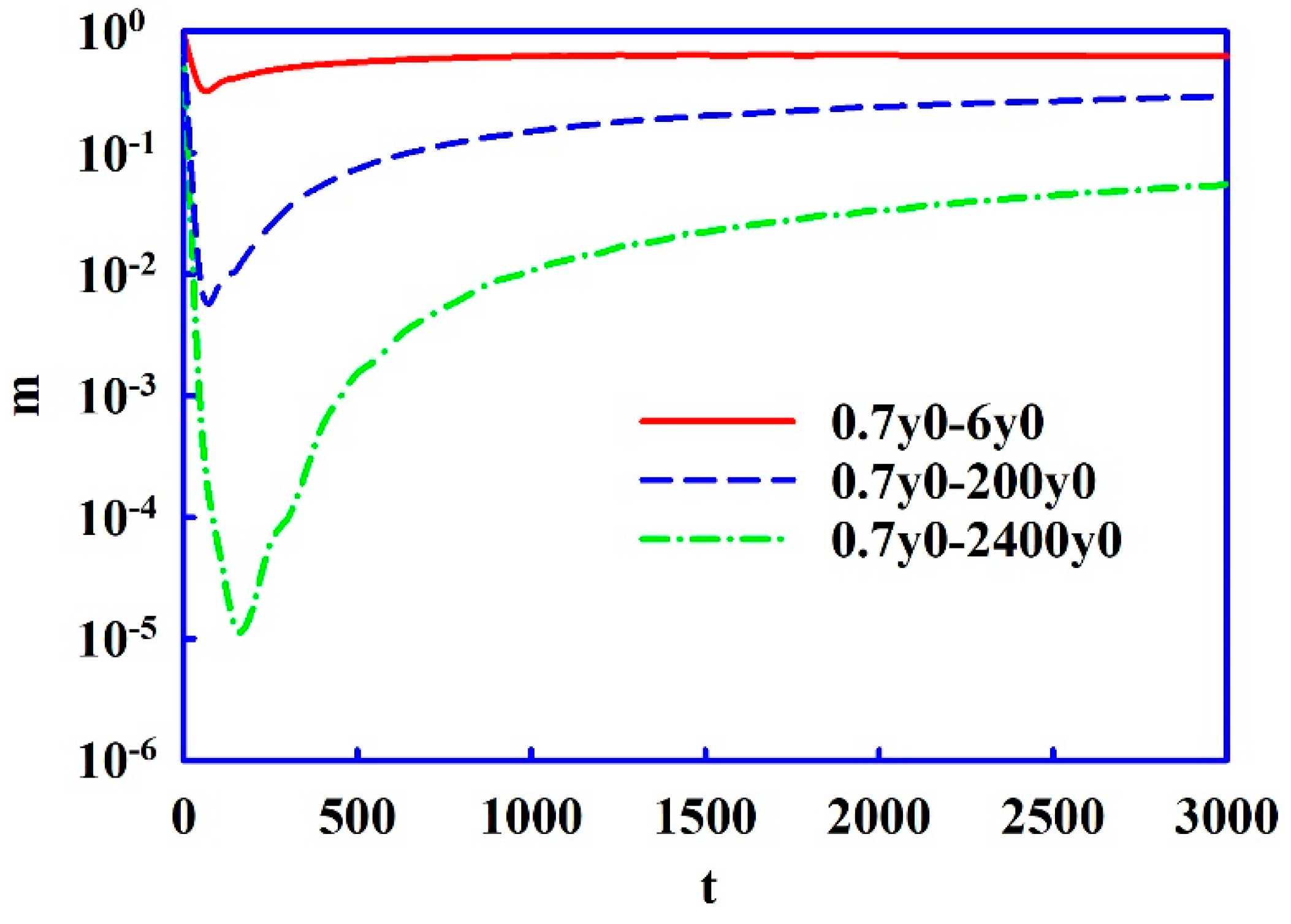
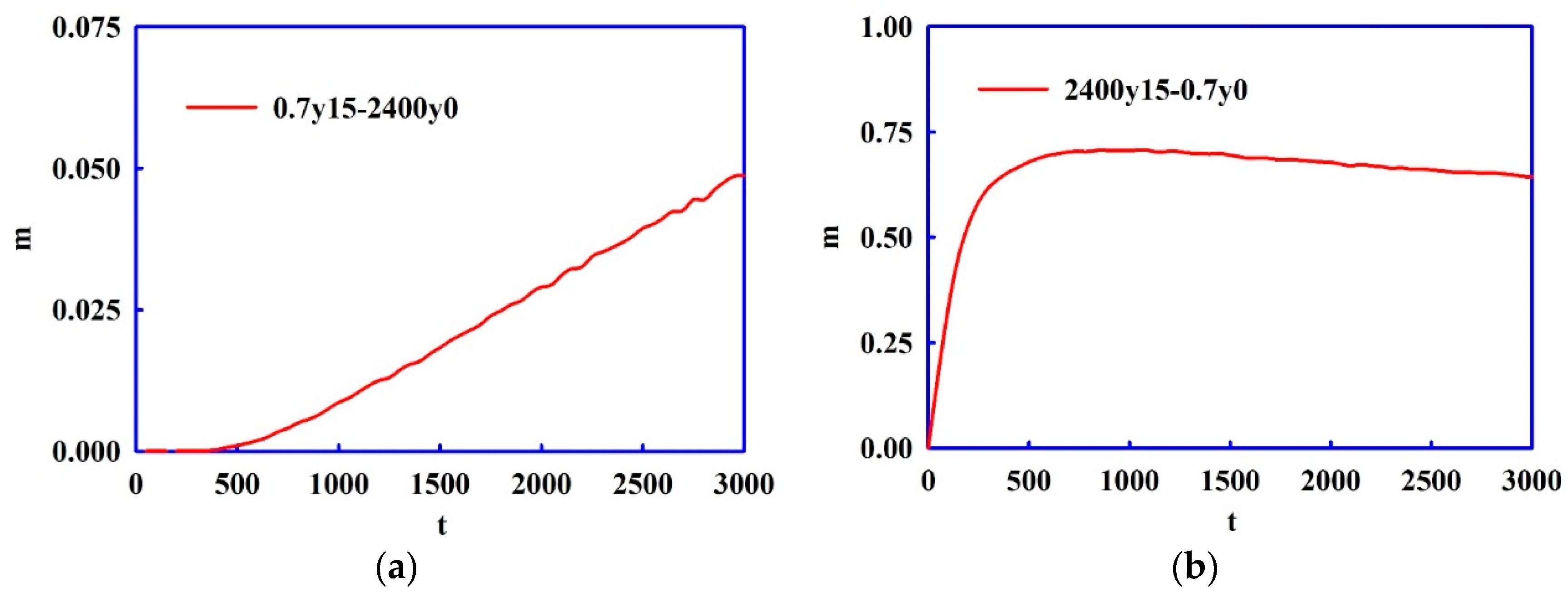
Figure 9 is a plot of the change of m for two puffs that have different Sc values. Puff A is the same as above, but puff B is a puff of drastically higher Sc, with a value of Sc = 2400. Figure 10 is a plot of the change of m for two puffs released at the same time at the wall of the channel. While the Sc of puffs released in the center region of the channel might not be that important in determining the dynamics of the mixing region, the Sc effects for puffs released in the viscous region close to the channel walls are important. In this region, the dynamics of the puff are affected by convection and by molecular diffusion. Figure 11 is a plot of m for two puffs that were released either with the high Sc puff released at the wall or the low Sc released at y_o = 15 (puff A is 0.7y15 and puff B is 2400y0) and for two puffs with the Sc reversed (puff is 2400y15 and puff B is 0.7y0).

4. Discussion

For the mixing of puffs of the same Sc released at different distances from the wall, it is seen in Figure 2 and Figure 3 that the mixing region starts from a crescent shape and slowly extends to cover the whole channel width. The crescent-shaped mixing region occurs because it represents the overlap region between puff A (released at the center of the channel and convecting downstream with a high velocity) and puff B (which is released at the logarithmic layer, where the mean flow velocity is less than at the channel centerline). The crescent shape is more pronounced in Figure 3, when one of the two mixing puffs is released closer to the wall (at y_o = 15). In Figure 12, we plot the individual puffs that resulted from the mixing shown in Figure 3a. One can see that the shape of the mixing region is the result of the shape of the individual puffs, and that the relative velocity of the puffs to each other and the shape of each puff (which is never a circle or an ellipse) play a very significant role in the dynamics of the mixing region. In anisotropic turbulence, such as the case of puffs released in a channel flow, mixing is affected by viscous effects and molecular diffusion, since the puff shape is the result of the interplay between molecular and convective transfer. At longer times, times larger than t = 2000 viscous wall units, the mixing region looks more homogenous, and the extent of it is quite large (see, for example, in Figure 3d, that the mixing region extends from roughly x = 50,000 to x = 54,000).

In Figure 4, it is seen that the Sc for the puff released in the viscous layer plays a role in the development of the mixing region, since the puff for higher Sc stays close to the channel wall for a longer time (note that the molecular diffusion for a high Sc puff is small, so that it takes longer for particles released close to the wall to get to the outer region of the flow field and mix with a puff released from the channel center). In Figure 4, it is seen that the crescent shape is narrower and the development of a mixing region that extends across the channel takes longer than seen in Figure 3.

The index for mixing quality ϕ, as introduced in Equation (5), at t = 500, offers more insights to the mixing process. While the mixing zone, which is mostly located in the lower half of the channel at this time, seems to be homogeneous in terms of mixing intensity (see Figure 1a), the quality of mixing is not the same across this area, with peak mixing quality at the semicircular region clearly seen in Figure 4a. Similar results are seen for the other cases considered. The intensity of mixing and the mixing location do not necessarily imply a high mixing quality, when one considers Figure 2, Figure 3 and Figure 4 along with their counterparts, Figure 5, Figure 6 and Figure 7. In theory, if the mixing intensity reaches a maximum value of 100%, then based on our previous definitions, the mixing quality will also reach a value of 0.25 at every mixing bin, implying that mixing is homogenous across the channel. However, mixing intensity cannot necessarily reach 100% (as in this study, the measurements showed that up to 70% of the total number of particles can be mixed), and a rather extended amount of time may be required for it to happen, assuming that there is no reaction between different types of particles during this period of time. Under this circumstance, the mixing quality index allows us to evaluate the mixing zone in terms of its homogeneity. From the observed values of this index, it may not be accurate to assume that perfect mixing always occurs in turbulent flow. One case where such effects could be more pronounced is in the case of a fast chemical reaction happening, where one reactant may be fully depleted. For example, if puffs A and B represent two reactants that react with one molecule of A reacting with one molecule of B, then the reaction will occur in the pattern seen in Figure 5, Figure 6 and Figure 7, where mixing is most homogeneous. If the reaction is exothermic, heat will be released in locations that follow the same pattern. This information might be important for the design and performance of chemical reactors in engineering, where controlling the reaction rate/location and heat transfer during the process is of high priority.

In a previous study [57], a mixing parameter was defined to quantify mixing that happens due to a Richtmyer-Meshkov instability, which involves the motion of two fluids with different densities driven by an impulsive acceleration. This parameter was said to be a measure for a fast reaction rate where one reactant is fully depleted, and the amount of mixing was quantified by measuring volume fractions along the x direction. The normalized mixing efficiency that is introduced here, depicted in Figure 8, Figure 9, Figure 10 and Figure 11, is a measure that considers both mixing intensity and quality of mixing in both x and y directions. It is seen that given the conditions prescribed in the simulations, there appears to be a maximum m for each pair of puffs. This maximum is approached asymptotically, and it indicates that the best mixing (m = 1) is not achieved. It is seen in Figure 8 and Figure 9 that the mixing is better when the two puffs are released in locations that are closer (see that m asymptotically goes to larger values when puff B is closer to the channel center). However, less mixing occurs when one puff is released at the center of the channel and the other at the channel wall, because the puff released at the wall is more elongated in the x direction. In Figure 9, where there is a large difference between the Sc of the two puffs, there is hardly any mixing when the second puff is released at the channel wall (see the green curve in Figure 9). When the Sc of puff B changes from 0.7 to 2400, there are no significant changes in the maximum m obtained when puff B is released at y_o = 75. The same is true when puff B is released at y_o = 15 (see Figure 8 and Figure 9). The values of m exhibit differences when puff B is released from the channel wall. Furthermore, when two puffs of significantly different Sc values are released from the wall of the channel, even when they are released at the same time and at the same location on the wall, the value of m starts at its maximum value of 1, then decreases to a minimum, and then increases again. The local minimum of m indicates a decrease in mixing–in other words, particles released together separate first and mix again later in the channel. This is a behavior that has been observed and analyzed recently [58,59] for small times, while here, it is clearly observed during a larger time interval.

The mixing behavior observed for the puffs examined in Figure 11 is quite interesting and might have implications for the design of reactors. The same two puffs are released in the flow field, but the Sc of the two puffs is switched. When the low Sc puff is released at the channel wall, large molecular diffusion helps to disperse the puff in the flow field and to reach the regions where the y_o = 15 puff reaches. Mixing occurs in that case, as seen by the value of m that is relatively high at long times (m goes to 0.64 asymptotically). However, when the high Sc puff is released from the channel wall, there is hardly any mixing between the two puffs. One would expect to observe this behavior given the details of the development of puffs released from the channel wall, and given the transition of the puff from molecular diffusion-dominated development to convection-dominated dispersion [58]. However, if one were to predict mixing behavior without a deeper appreciation of the molecular effects on turbulent dispersion in anisotropic turbulence, the predictions might not have been correct.

5. Conclusions

Mixing in an anisotropic turbulent velocity field generated by channel flow has been studied using Lagrangian methods (direct numerical simulation of turbulent flow and Lagrangian scalar tracking techniques). Measures that quantify the efficiency of mixing in terms of both quality and intensity have been introduced and utilized to explore the simulation results. It is found that the mixing of puffs released in the flow field can depend strongly on the Schmidt number and on the location of puff release. It is also found that only calculating how many particles are mixed is not enough to obtain a full picture of the process, which is completed when the quality of mixing is taken into account. While the Sc of the puff released at the center of the flow field is not critical to the mixing process (as has previously been shown) it is now found that the Sc of puffs released at the wall or in the viscous wall region is important. Finally, it appears that one could control particle mixing and particle separation as a function of time after particle release by determining the position of puff injection in the flow field. This realization could be taken advantage of in the design of equipment for applications where the control of mixing is important. While the results presented here are obtained for passive scalar and cannot be extended to non-passive particles, one could change the equation of motion of the particles and include effects like drag, lift etc., to apply a similar analysis for non-passive particles.

References

- Tennekes, H.; Lumley, J.L. A First Course in Turbulence; MIT Press: Boston, MA, USA, 1972. [Google Scholar]
- Dimotakis, P.E. Turbulent Mixing. Annu. Rev. Fluid Mech. 2005, 37, 329–356. [Google Scholar] [CrossRef]
- Fox, R.O. Computational Models for Turbulent Reacting Flows; Cambridge University Press: Cambridge, UK, 2003. [Google Scholar]
- Curl, R.L. Dispersed phase mixing: I. Theory and effects in simple reactors. AlChE J. 1963, 9, 175–181. [Google Scholar] [CrossRef]
- Subramaniam, S.; Pope, S.B. A mixing model for turbulent reactive flows based on Euclidean minimum spanning trees. Combust. Flame 1998, 115, 487–514. [Google Scholar] [CrossRef] [Green Version]
- Oldshue, J.W. Fluid Mixing Techology; McGraw Hill: New York, NY, USA, 1983. [Google Scholar]
- Paul, E.L.; Atiemo-Obeng, V.A.; Kresta, M.S. Handbook of Industrial Mixing: Science and Practice; John Wiley & Sons: Hoboken, NJ, USA, 2004. [Google Scholar]
- Mylne, K.R.; Mason, P.J. Concentration fluctuation measurements in a dispersing plume at a range of up to 1000 m. QJRMS 1991, 117, 177–206. [Google Scholar] [CrossRef]
- Pasquill, F.; Smith, F.B. Atmospheric Diffusion; Horwood, E., Ed.; John Wiley & Sons: Hoboken, NJ, USA, 1983; p. 437. [Google Scholar]
- Ottino, J.M. The Kinematics of Mixing: Stretching, Chaos, and Transport; Cambridge University Press: Cambridge, UK, 1989. [Google Scholar]
- Kukukova, A.; Aubin, J.; Kresta, S.M. A new definition of mixing and segregation: Three dimensions of a key process variable. Chem. Eng. Res. Des. 2009, 87, 633–647. [Google Scholar] [CrossRef] [Green Version]
- Calzavarini, E.; Cencini, M.; Lohse, D.; Toschi, F. Quantifying Turbulence-Induced Segregation of Inertial Particles. Phys. Rev. Lett. 2008, 101, 084504. [Google Scholar] [CrossRef] [PubMed]
- Green, D.W.; Perry, R.H. Perry’s Chemical Engineers’ Handbook, 8th ed.; McGraw Hill: New York, NY, USA, 2007. [Google Scholar]
- Papavassiliou, D.V. Turbulent transport from continuous sources at the wall of a channel. Int. J. Heat Mass Transf. 2002, 45, 3571–3583. [Google Scholar] [CrossRef]
- Hanratty, T.J. Heat transfer through a homogeneous isotropic turbulent field. AlChE J. 1956, 2, 42–45. [Google Scholar] [CrossRef]
- Papavassiliou, D.V.; Hanratty, T.J. Transport of a passive scalar in a turbulent channel flow. Int. J. Heat Mass Transf. 1997, 40, 1303–1311. [Google Scholar] [CrossRef]
- Mitrovic, B.M.; Le, P.M.; Papavassiliou, D.V. On the Prandtl or Schmidt number dependence of the turbulent heat or mass transfer coefficient. Chem. Eng. Sci. 2004, 59, 543–555. [Google Scholar] [CrossRef]
- Incropera, F.P.; Kerby, J.S.; Moffatt, D.F.; Ramadhyani, S. Convection heat transfer from discrete heat sources in a rectangular channel. Int. J. Heat Mass Transf. 1986, 29, 1051–1058. [Google Scholar] [CrossRef]
- Raupach, M.R.; Legg, B.J. Turbulent dispersion from an elevated line source—Measurements of wind concentration moments and budgets. J. Fluid Mech. 1983, 136, 111–137. [Google Scholar] [CrossRef]
- Poreh, M.; Cermak, J.E. Study of diffusion from a line source in a turbulent boundary layer. Int. J. Heat Mass Transf. 1964, 7, 1083–1095. [Google Scholar] [CrossRef]
- Fackrell, J.E.; Robins, A.G. Concentration fluctuations and fluxes in plumes from point sources in a turbulent boundary layer. J. Fluid Mech. 1982, 117, 1–26. [Google Scholar] [CrossRef]
- Shlien, D.J.; Corrsin, S. Dispersion measurements in a turbulent boundary layer. Int. J. Heat Mass Transf. 1976, 19, 285–295. [Google Scholar]
- Beguier, C.; Dekeyser, I.; Launder, B.E. Ratio of scalar and velocity dissipation time scales in shear flow turbulence. Phys. Fluids 1978, 21, 307–310. [Google Scholar] [CrossRef]
- Ma, B.K.; Warhaft, Z. Some aspects of the thermal mixing layer in grid turbulence. Phys. Fluids 1986, 29, 3114–3120. [Google Scholar] [CrossRef]
- Dahm, W.J.A.; Dimotakis, P.E. Mixing at large Schmidt number in the self-similar far field of turbulent jets. J. Fluid Mech. 1990, 217, 299–330. [Google Scholar] [CrossRef]
- Yeung, P.K.; Xu, S. Schmidt number effects on turbulent transport with uniform mean scalar gradient. Phys. Fluids 2002, 14, 4178–4191. [Google Scholar] [CrossRef]
- Borgas, M.S.; Sawford, B.L.; Xu, S.; Donzis, D.A.; Yeung, P.K. High Schmidt number scalars in turbulence: Structure functions and Lagrangian theory. Phys. Fluids 2004, 16, 3888–3899. [Google Scholar] [CrossRef]
- Buaria, D.; Yeung, P.K.; Sawford, B.L. A Lagrangian study of turbulent mixing: Forward and backward dispersion of molecular trajectories in isotropic turbulence. J. Fluid Mech. 2016, 799, 352–382. [Google Scholar] [CrossRef]
- Yeung, P.K.; Donzis, D.A. High-Reynolds-number simulation of turbulent mixing. Phys. Fluids 2005, 17, 081703. [Google Scholar] [CrossRef]
- Sawford, B.L. Lagrangian modeling of scalar statistics in a double scalar mixing layer. Phys. Fluids 2006, 18, 085108. [Google Scholar] [CrossRef]
- Sawford, B.L.; Kops, S.M.D.B. Direct numerical simulation and Lagrangian modeling of joint scalar statistics in ternary mixing. Phys. Fluids 2008, 20, 095106. [Google Scholar] [CrossRef]
- Brethouwer, G.; Hunt, J.C.R.; Nieuwstadt, F.T.M. Micro-structure and Lagrangian statistics of the scalar field with a mean gradient in isotropic turbulence. J. Fluid Mech. 2003, 474, 193–225. [Google Scholar] [CrossRef]
- Yeung, P.K.; Xu, S.; Donzis, D.A.; Sreenivasan, K.R. Simulations of three-dimensional turbulent mixing for Schmidt numbers of the order 1000. Flow Turbul. Combust. 2004, 72, 333–347. [Google Scholar] [CrossRef]
- Srinivasan, C.; Papavassiliou, D.V. Heat Transfer Scaling Close to the Wall for Turbulent Channel Flows. Appl. Mech. Rev. 2013, 65. [Google Scholar] [CrossRef]
- Srinivasan, C.; Papavassiliou, D.V. Prediction of the turbulent Prandtl number in wall flows with Lagrangian simulations. Ind. Eng. Chem. Res. 2011, 50, 8881–8891. [Google Scholar] [CrossRef]
- Srinivasan, C.; Papavassiliou, D.V. Comparison of backwards and forwards scalar relative dispersion in turbulent shear flow. Int. J. Heat Mass Transf. 2012, 55, 5650–5664. [Google Scholar] [CrossRef]
- Hasegawa, Y.; Kasagi, N. Low-pass filtering effects of viscous sublayer on high Schmidt number mass transfer close to a solid wall. Int. J. Heat Fluid Flow 2009, 30, 525–533. [Google Scholar] [CrossRef]
- Mito, Y.; Hanratty, T.J. Lagrangian stochastic simulation of turbulent dispersion of heat markers in a channel flow. Int. J. Heat Mass Transf. 2003, 46, 1063–1073. [Google Scholar] [CrossRef]
- Koumoutsakos, P. Multiscale flow simulations using particles. Annu. Rev. Fluid Mech. 2005, 37, 457–487. [Google Scholar] [CrossRef]
- Moin, P.; Mahesh, K. Direct numerical simulation: A tool in turbulence research. Annu. Rev. Fluid Mech. 1998, 30, 539–578. [Google Scholar] [CrossRef]
- Lee, M.; Moser, R.D. Direct numerical simulation of turbulent channel flow up to Re-tau approximate to 5200. J. Fluid Mech. 2015, 774, 395–415. [Google Scholar] [CrossRef]
- Lyons, S.L.; Hanratty, T.J.; McLaughlin, J.B. Direct numerical simulation of passive heat transfer in a turbulent channel flow. Int. J. Heat Mass Transf. 1991, 34, 1149–1161. [Google Scholar] [CrossRef]
- Alfonsi, G. On Direct Numerical Simulation of Turbulent Flows. Appl. Mech. Rev. 2011, 64, 64. [Google Scholar] [CrossRef]
- Nguyen, Q.; Feher, S.E.; Papavassiliou, D.V. Lagrangian Modeling of Turbulent Dispersion from Instantaneous Point Sources at the Center of a Turbulent Flow Channel. Fluids 2017, 2. [Google Scholar] [CrossRef]
- Nguyen, Q.; Papavassiliou, D.V. Scalar mixing in anisotropic turbulent flow. AlChE J. 2018. [Google Scholar] [CrossRef]
- Lyons, S.L.; Hanratty, T.J.; McLaughlin, J.B. Large-scale computer simulation of fully developed turbulent channel flow with heat transfer. Int. J. Numer. Methods Fluids 1991, 13, 999–1028. [Google Scholar] [CrossRef]
- Gunther, A.; Papavassiliou, D.V.; Warholic, M.D.; Hanratty, T.J. Turbulent flow in a channel at a low Reynolds number. Exp. Fluids 1998, 25, 503–511. [Google Scholar] [CrossRef]
- Kontomaris, K.; Hanratty, T.J.; McLaughlin, J.B. An algorithm for tracking fluid particles in a spectral simulation of turbulent channel flow. J. Comput. Phys. 1992, 103, 231–242. [Google Scholar] [CrossRef]
- Mitrovic, B.M.; Papavassiliou, D.V. Transport properties for turbulent dispersion from wall sources. AlChE J. 2003, 49, 1095–1108. [Google Scholar] [CrossRef]
- Na, Y.; Papavassiliou, D.V.; Hanratty, T.J. Use of direct numerical simulation to study the effect of Prandtl number on temperature fields. Int. J. Heat Fluid Flow 1999, 20, 187–195. [Google Scholar] [CrossRef]
- Orszag, S.A.; Kells, L.C. Transition to turbulence in plane Poiseuille and plane Couette flow. J. Fluid Mech. 1980, 96, 159–205. [Google Scholar] [CrossRef]
- Marcus, P.S. Simulation of Taylor-Couette flow. 1. Numerical methods and comparison with experiment. J. Fluid Mech. 1984, 146, 45–64. [Google Scholar] [CrossRef]
- Einstein, A. Uber die von der molekular-kinetischen Theorie der Warme geforderte Bewegung von in ruhenden Flussigkeiten suspendierten Teilchen. Ann. Phys. 1905, 17, 549. [Google Scholar] [CrossRef]
- Papavassiliou, D.V.; Hanratty, T.J. The use of Lagrangian-methods to describe turbulent transport of heat from a wall. Ind. Eng. Chem. Res. 1995, 34, 3359–3367. [Google Scholar] [CrossRef]
- Saffman, P.G. On the effect of the molecular diffusivity in turbulent diffusion. J. Fluid Mech. 1960, 8, 273–283. [Google Scholar] [CrossRef]
- Le, P.M.; Papavassiliou, D.V. Turbulent Dispersion from Elevated Line Sources in Channel and Couette Flow. AlChE J. 2005, 51, 2402–2414. [Google Scholar] [CrossRef]
- Thornber, B.; Drikakis, D.; Youngs, D.L.; Williams, R.J.R. The influence of initial conditions on turbulent mixing due to Richtmyer-Meshkov instability. J. Fluid Mech. 2010, 654, 99–139. [Google Scholar] [CrossRef]
- Nguyen, Q.; Srinivasan, C.; Papavassiliou, D.V. Flow-induced separation in wall turbulence. Phys. Rev. E 2015, 91, 033019. [Google Scholar] [CrossRef] [PubMed]
- Nguyen, Q.; Papavassiliou, D.V. A statistical model to predict streamwise turbulent dispersion from the wall at small times. Phys. Fluids 2016, 28, 125103. [Google Scholar] [CrossRef]
Figure 1.
Channel geometry and points of release of markers at time t = 0.
Figure 2.
Development of the mixing region with time for two puffs, puff A: Sc = 0.7, yo = 300, and puff B: Sc = 0.7, yo = 75. (a) Contours of nAB at t = 500; (b) Contours of nAB at t = 1000; (c) Contours of nAB at t = 2000; (d) Contours of nAB at t = 3000.
Figure 3.
Development of the mixing region with time for two puffs, puff A: Sc = 0.7, yo = 300, and puff B: Sc = 0.7, yo = 15. (a) Contours of nAB at t = 500; (b) Contours of nAB at t = 1000; (c) Contours of nAB at t = 2000; (d) Contours of nAB at t = 3000.
Figure 4.
Development of the mixing region with time for two puffs, puff A: Sc = 0.7, yo = 300, and puff B: Sc = 2400, yo = 15. (a) Contours of nAB at t = 500; (b) Contours of nAB at t = 1000; (c) Contours of nAB at t = 2000; (d) Contours of nAB at t = 3000.
Figure 5.
Mixing efficiency in the flow channel based on the contours of the mixing quality index, ϕ, for two puffs, puff A: Sc = 0.7, yo = 300, and puff B: Sc = 0.7, yo = 75. (a) Contours of ϕ at t = 500; (b) at t = 1000; (c) at t = 2000; and (d) at t = 3000.
Figure 6.
Mixing efficiency in the flow channel based on the contours of the mixing quality index, ϕ, for two puffs, puff A: Sc = 0.7, yo = 300, and puff B: Sc = 0.7, yo = 15. (a) Contours of ϕ at t = 500; (b) at t = 1000; (c) at t = 2000; and (d) at t = 3000.
Figure 7.
Mixing efficiency in the flow channel based on the contours of the mixing quality index, ϕ, for two puffs, puff A: Sc = 0.7, yo = 300, and puff B: Sc = 2400, yo = 15. (a) Contours of ϕ at t = 500; (b) at t = 1000; (c) at t = 2000; and (d) at t = 3000.
Figure 8.
Normalized mixing efficiency m for mixing between a puff released at the channel center (puff A: Sc = 0.7, yo = 300) and puffs of the same Sc released at distances yo = 75, 15, and 0.
Figure 9.
Normalized mixing efficiency m for mixing between a puff released at the channel center (puff A: Sc = 0.7, yo = 300) and puffs of drastically different Sc values (Sc = 2400) released at distances yo = 75, 15, and 0.
Figure 10.
Normalized mixing efficiency m for mixing between two puffs released at the channel wall, but with different Schmidt numbers (here we have all 4 Sc).
Figure 11.
Normalized mixing efficiency m for mixing between two puffs released at the channel wall, and at y = 15, but with Schmidt numbers switching between the two configurations ((a): mixing between puff 0.7y15 and puff 2400y0, (b): mixing between puff 2400y15 and puff 0.7y0).
Figure 12.
Contours of the location of the two puffs mixing at t = 500, corresponding to the conditions of Figure 3a. (a) Puff A (Sc = 0.7, yo = 300), and (b) Puff B (Sc = 0.7, yo = 15). Note that the shape of puff B is elongated in the streamwise direction and a large part of it is close to the wall. The shape of puff A looks like a jellyfish, because of the high mean velocity at the channel center. Mixing occurs at the overlap of these two puffs.
© 2018 by the authors. Licensee MDPI, Basel, Switzerland. This article is an open access article distributed under the terms and conditions of the Creative Commons Attribution (CC BY) license (http://creativecommons.org/licenses/by/4.0/).
Share and Cite
MDPI and ACS Style
Nguyen, Q.; Papavassiliou, D.V. Quality Measures of Mixing in Turbulent Flow and Effects of Molecular Diffusivity. Fluids 2018, 3, 53. https://doi.org/10.3390/fluids3030053
AMA Style
Nguyen Q, Papavassiliou DV. Quality Measures of Mixing in Turbulent Flow and Effects of Molecular Diffusivity. Fluids. 2018; 3(3):53. https://doi.org/10.3390/fluids3030053
Chicago/Turabian StyleNguyen, Quoc, and Dimitrios V. Papavassiliou. 2018. "Quality Measures of Mixing in Turbulent Flow and Effects of Molecular Diffusivity" Fluids 3, no. 3: 53. https://doi.org/10.3390/fluids3030053