Encapsulation of Droplets Using Cusp Formation behind a Drop Rising in a Non-Newtonian Fluid

Abstract

The rising of a Newtonian oil drop in a non-Newtonian viscous solution is studied experimentally. In this case, the shape of the ascending drop is strongly affected by the viscoelastic and shear-thinning properties of the surrounding liquid. We found that the so-called velocity discontinuity phenomena is observed for drops larger than a certain critical size. Beyond the critical velocity, the formation of a long tail is observed, from which small droplets are continuously emitted. We determined that the fragmentation of the tail results mainly from the effect of capillary effects. We explore the idea of using this configuration as a new encapsulation technique, where the size and frequency of droplets are directly related to the volume of the main rising drop, for the particular pair of fluids used. These experimental results could lead to other investigations, which could help to predict the droplet formation process by tuning the two fluids’ properties, and adjusting only the volume of the main drop.

1. Introduction

The problem of encapsulating droplets of fluid has important implications in the fields of bioengineering and medical research, for instance to encapsulate cells [1]. With the development of microfluidics and lab-on-chip technology to perform analysis on different fluids, the dynamics and size of such droplets have to be well controlled [2,3,4]. Several techniques have been used to perform such encapsulation, for instance using a T-junctions device [5,6]. To be able to perform such encapsulation at a larger scale in a controlled matter still remains to be achieved.

Here, we study a new alternative technique to encapsulate oil drops by using the non-Newtonian properties of the surrounding liquid. In the case of an object rising or falling in a non-Newtonian fluid, new and unexpected phenomena appear in comparison with the Newtonian case. The flow surrounding the object can be highly modified, due to the viscoelastic properties of the fluids [7,8,9,10,11,12,13].

It has been observed that when a bubble or a drop moves, as a result of gravity, in a viscoelastic shear-thinning fluid, a velocity discontinuity phenomenon appears [14,15,16,17,18,19]. When the bubble or drop reaches a certain critical size, its terminal speed increases sharply. The sudden increase has not been understood fully until recently [17]: a combination of effects has to occur simultaneously. First the viscoelastic nature of the outside liquid induces a change in shape of the drop or bubble, forming a characteristic cusped shape [14,15,19,20,21]; resulting from this change of shape, the drag coefficient of the object is reduced. Consequently, the speed increases, which, given the shear-thinning properties, will cause the viscosity around the object to decrease, causing an even further rising velocity increase. This set of features was recently discussed by [17] in detail. Recent numerical simulations have helped to clarify the connection among these behaviours [22].

Furthermore, when the velocity discontinuity appears, a negative wake behind the object is also detected. The flow field behind the bubble reverses direction. This phenomenon was first observed by [23] and was directly related to the appearance of the velocity discontinuity by [14,19,22].

More interestingly, for the case of a drop, a recent study by [20] found that a long thin tail formed from the cusp at the rear edge of the drop. This long tail became unstable, fragmenting into small droplets that were then left behind the main drop. They observed the tail formation and fragmentation when the external fluid had non-Newtonian properties. Since they conducted experiments with both Newtonian (as in the present case) and non-Newtonian drops, it was possible to determine that viscoelastic drops formed much longer and thicker tails than the Newtonian case. It is important to note that the fragmentation of the tail was not analyzed in detail. This is, in fact, one of the objectives of the present study. The fragmentation of fluid filaments has been extensively studied in the literature under different flow conditions [24,25]. For the case of viscoelastic filament, the breakup has been shown to lead to the formation of bead-on-a-string [26,27]. In most cases, the fragmentation results from capillary-driven instabilities similar to the Rayleigh–Plateau instability [24,25]. Some studies have addressed the case of a Newtonian jet flowing from a nozzle in a viscoelastic fluid [28,29,30]. In those experiments, the jet fragmenting is controlled by the injection flow, while, in the present case, the filament is created directly by the rising drop.

In this article, we present results on the formation of droplets behind an oil drop (Newtonian) rising in a water/glycerol-polyacrylamide solution (non-Newtonian). First, we present the experimental set-up and a characterization of the fluids we used. Then, we present the experimental observations, and the different regimes of breakup that were observed. Finally, we discuss different aspects of the droplets formation, by relating the velocity and volume of the main drop, the size of the tail appearing behind the drop and the size and frequency of formation of the droplets. These results, obtained only for a single pair of Newtonian/non-Newtonian fluids, could lead to a more extensive investigation with which this phenomenon could be fully understood.

2. Experimental Set-Up and Test Fluids

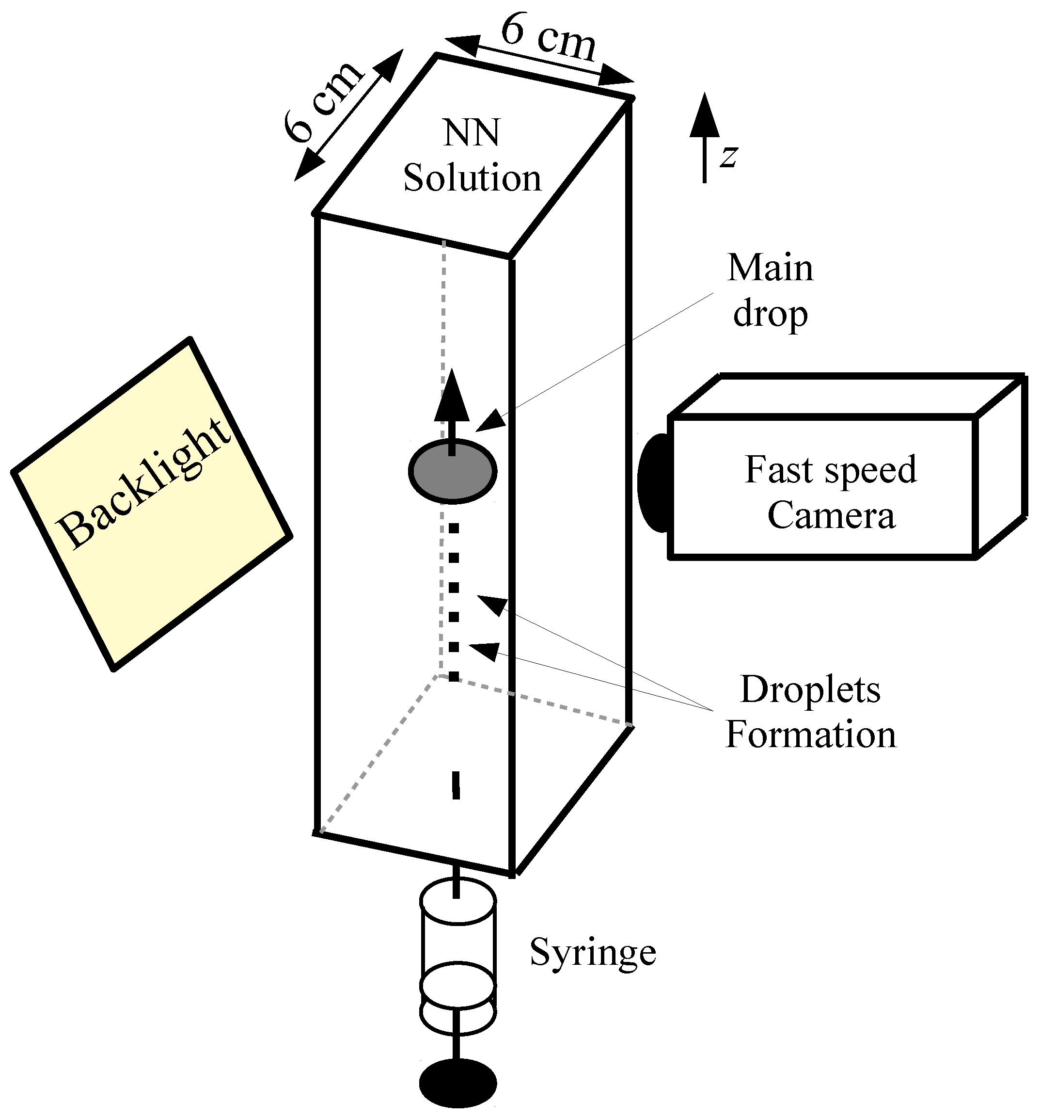
The experimental setup consists of a vertical glass column of a height 60 cm (Figure 1). This column is square based with a side width of 6 cm. This column is wide enough so that wall effects are negligible on the drop dynamics, as the velocity field decreases rapidly with the distance to the drop. The setup is filled with a non-Newtonian water-polyacrylamide solution. Alimentary corn oil is injected at the bottom of the column using a plastic syringe with a volume capacity of 5 mL. The set-up is backlit with a LED panel. A fast speed camera (SpeedSence, Phantom) films the rising at a frequency of 200 frames per seconds with a resolution 1632 × 1200 during 10 s. The camera is placed at mid height of the column and films a zone of about 12 cm high. At this point, the drop moves at its terminal speed. The scale ratio of the images is of 110 pixels per centimeter, and we measure the diameter, height and position of the drop with a precision of about two pixels, so the error is estimated to be smaller than 5 percent for the drop velocity and volume (see Section 3). The error bars have been reported on the different figures.

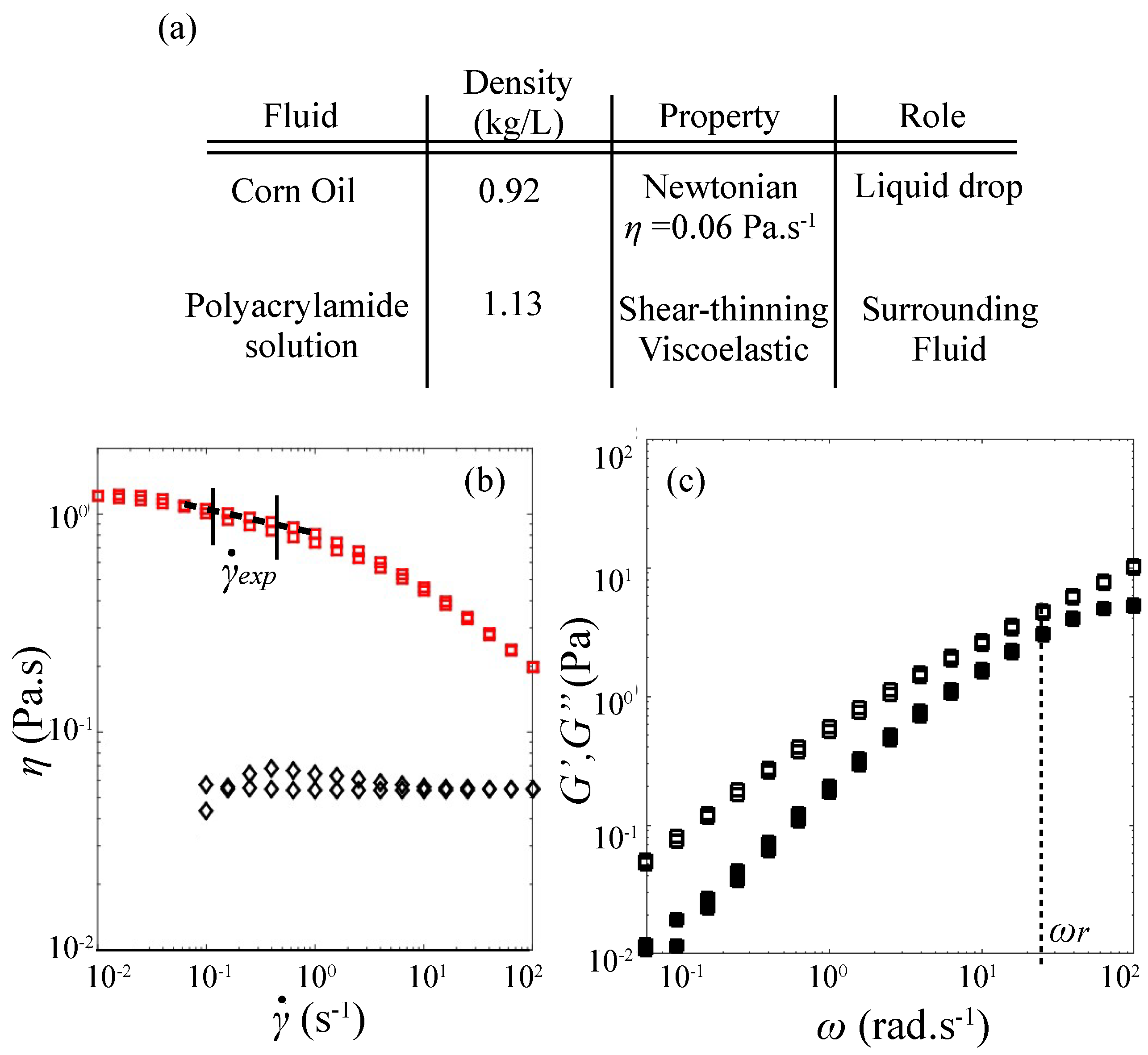
The properties of the two fluids used are presented in Figure 2a. The drop consists in an alimentary corn oil, characterized as Newtonian. For the surrounding fluid, we used a solution composed of a 49.75% weight solution of water and glycerol each and 0.5% of industrial polyacrylamide (PAAM, Separan) which are long chains of polymer. This high concentration ensures that the non-Newtonian behaviour of the fluid will be important (shear-thinning and viscoelasticity). The density was measured using a flask with a precise volume of 25 mL, which was filled with the different fluids and weighed.

Both fluids were characterized using a rheometer (HR, TA Instruments), and we performed two types of tests. We used a plane–plane geometry with a gap of 1 mm, at a fixed temperature of 25 °C and we measured the viscosity, varying the shear-rate. The shear rate $\dot{\gamma }$ is varied from 0.01 to 100 s⁻¹ for the polymer solution and from 0.1 to 100 s⁻¹ for the oil with five points per decade (for the oil, the rheometer does not have sufficient accuracy for $\dot{\gamma }<0.01$ s⁻¹ because of the low viscosity), with an averaging time of 30 s for each point, and with back and forth variation for reproducibility (going from low shear rate to high, and then reverse). The results are presented in Figure 2b. We observe that the corn oil is Newtonian, with a viscosity ${\eta }_{oil}\approx 0.06$ Pa.s. The non-Newtonian fluid, shows a shear-thinning behaviour, as the viscosity ${\eta }_{PAAM}$ (red squares) decreases with the shear rate $\dot{\gamma }$. In our case, the shear-rates when the drop ascends in a range between $\dot{\gamma }=0.22$ s⁻¹ and $\dot{\gamma }=0.42$ s⁻¹. In this zone, the viscosity follows a power law: $\eta =K{\dot{\gamma }}^{n-1}$, where $n=0.87$ and $K=1.10$ as represented in Figure 2b. This type of decrease is typical for polyacryalimde solutions [31,32]. This exponent n being close to 1 (Newtonian behaviour for $n=1$) indicates that the shear-thinning is insignificant in our experiment. The important decrease in viscosity $\eta$ will appear for shear-rates $\dot{\gamma }$ higher than those relevant here.

For the non-Newtonian solution, an oscillatory test was also performed. A deformation of 3% was imposed, and the frequency of oscillation $\omega$ was varied from 0.06 to 100 rad·s⁻¹ during two periods for each point. With these measurements, the elastic $G^{\prime }$ (empty symbols) and viscous modulus $G^{″}$ (filled symbols) are obtained. We observe a viscoelastic behaviour, where the elastic property is dominant at a low shear rate. This is in agreement with what has already been observed for such polymer solutions [32]. The relaxation time can be approximated as the time where the two moduli are equal and represents the typical time where the non-Newtonian fluid goes from an elastic solid behaviour to a viscous fluid. This is represented in Figure 2c as ${\omega }_r=25$ rad·s⁻¹, and we estimate the relaxation time ${\tau }_r=2\pi /{\omega }_r=0.25$ s.

3. Experimental Observations: Different Regimes

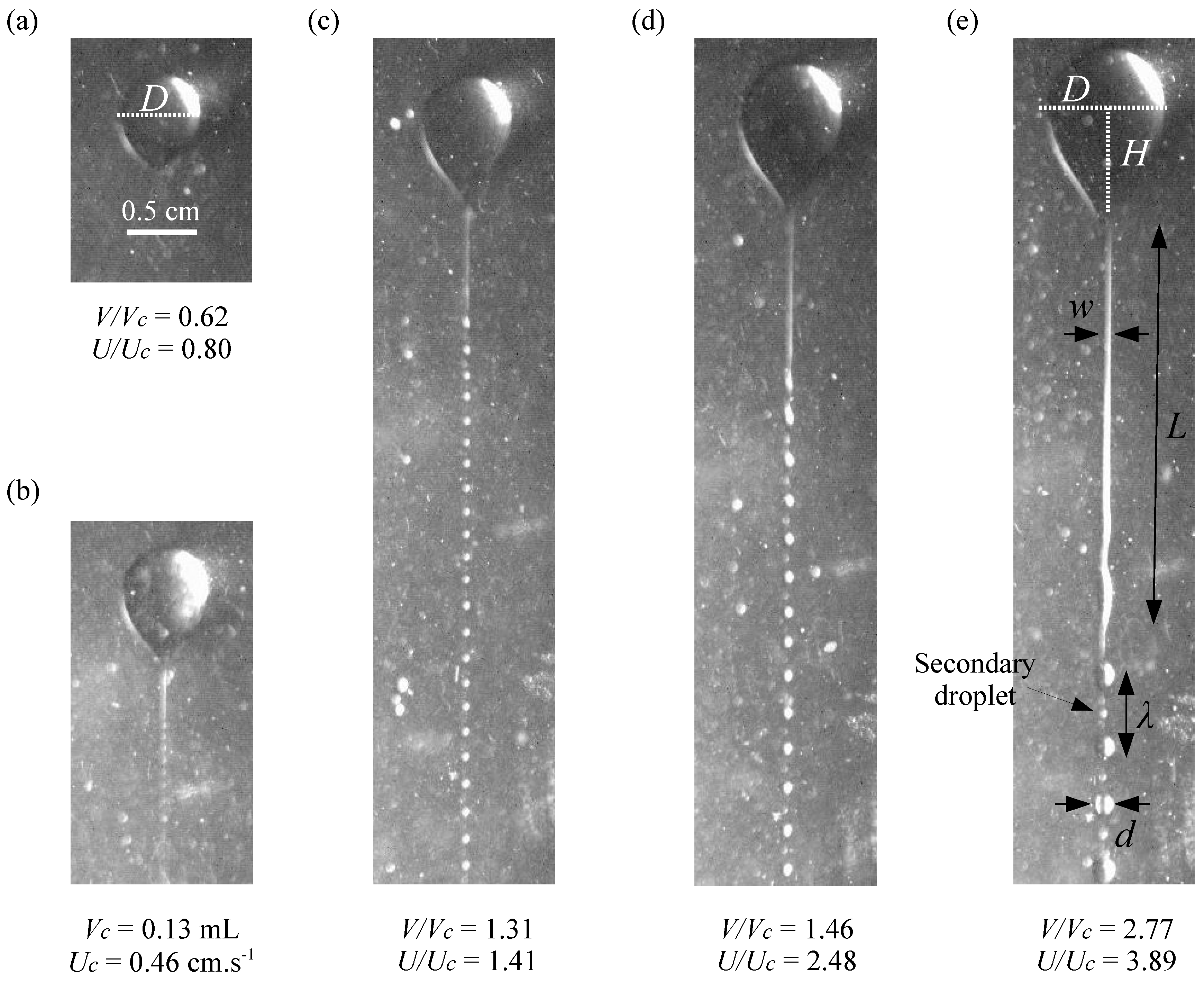
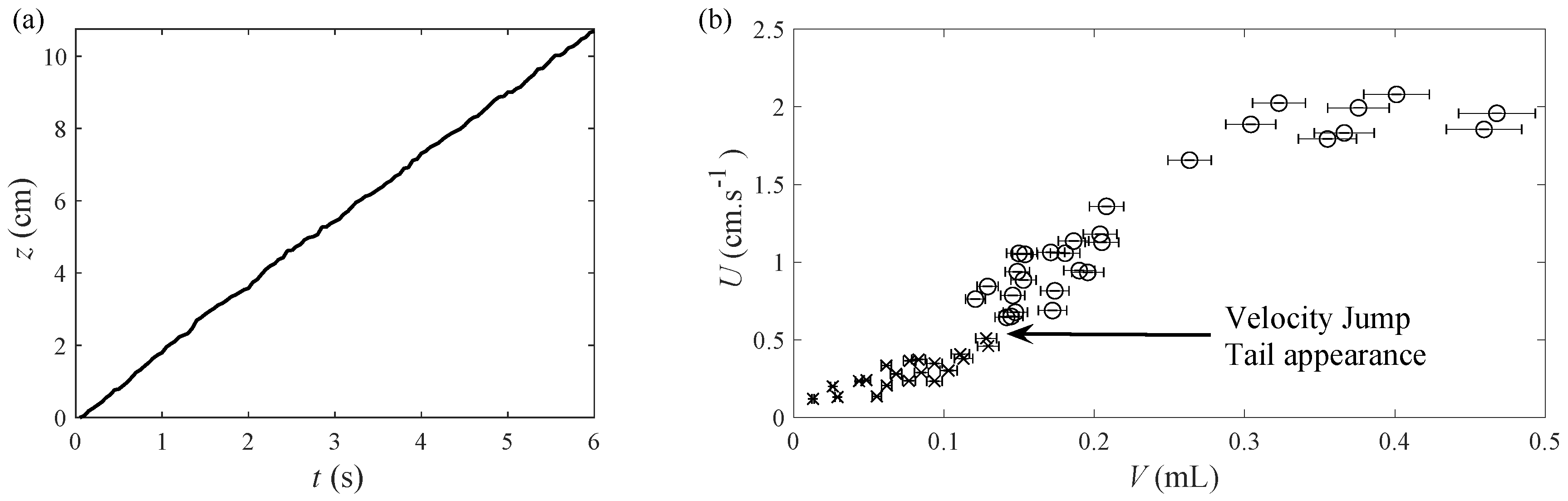
The experiment is performed by injecting oil at the bottom of the fluid column, using a plastic syringe. The oil volume V is not measured a priori, instead it is estimated by image analysis, considering that, for small drops, the volume corresponds to the one of a sphere of diameter D:$V=\pi D^3/6$ (Figure 3a), and, for the bigger ones, it is the sum of a cone of height H and a hemisphere of diameter D:$V=\pi D^{2}H/12+\pi D^3/12$ (Figure 3b–e). To ensure good statistics, we reproduce the experiment 50 times varying the volume V from 0.01 to 0.47 mL. We detect the position of the front of the drop to determine its velocity. Figure 4a presents the evolution of the vertical position z of the front of the drop as a function of time t for a drop of volume $V=0.36$ mL. For all drops, we observe that the vertical position is linear in time t; the rising velocity U is computed by a simple linear regression. Figure 4b shows the rising velocity U of the drop as a function of its volume V. The rising velocity increases slowly with the volume until it reaches a critical volume ($V_c=0.13$ mL). At this volume, a small velocity jump is observed, which has already been reported in literature as the velocity discontinuity [14,15,16,17,18,22]. This appears for bubbles and drops rising in a viscoelastic surrounding fluid, and is directly linked with the appearance of a negative wake behind the bubble/drop. Above the critical volume $V_c$, the rising velocity U increases more rapidly with the volume V. Considering the non-Newtonian properties of the surrounding fluid (shear-thinning and viscoelastic), it is not possible to predict the shape of the curve over this critical volume, but many other experimental examples have reported similar behaviour for drops or bubbles [14,20,21,23].

In terms of dimensionless numbers, it is common to use the Reynolds number Re and the Deborah number De. The Reynolds number compares the inertial forces of the flow with the viscous ones: $\mathrm{Re}=\rho UD/\eta =\rho UD/K{\dot{\gamma }}^{n-1}$, where $\rho$ is the density of the surrounding fluid, U the velocity of the drop, D the diameter of the drop and $\eta$ the viscosity. In our case, the fluid is shear thinning, so the viscosity changes with the shear rate. A common way to account for this problem is to define the shear-rate as the ratio of velocity and diameter of the drop $\dot{\gamma }=U/D$, and to use this in the rheological measurements using the formula $\eta =K{\dot{\gamma }}^{n-1}$ where $n=0.87$ and $K=1.10$ (see Section 2). We obtain a modified Reynolds number scaling as $\mathrm{Re}=U^{2-n}\rho D^n/K$ (see, for instance, [33]). This gives us a Reynolds number varying from 5$\times {10}^{-3}$ to 2.39. This small Reynolds number shows that inertial effects are small. The Deborah number compares the viscoelastic relaxation time and the observation time scale: $\mathrm{De}={\tau }_r/{\tau }_o$. We can define the observation time scale as the inverse of the shear rate: ${\tau }_o=1/\dot{\gamma }=D/U$ and the relaxation time is defined in Section 2: ${\tau }_r=2\pi /{\omega }_r=0.25$ s. In our experiment, we have the Deborah number varying from $5.6\times {10}^{-2}$ for the largest drops to $10.6\times {10}^{-2}$ for the smallest ones. This range of values indicates that elastics effects are small but not negligible. Note that experiments were conducted only with one container size. Since the Reynolds number is small, the walls will affect the terminal velocity of the drops. Considering the Faxen series correction (see Mendoza-Fuentes et al., [34]), the terminal velocity will be smaller by 51% for the case of the largest drop. Note that the correction is valid only for spherical particles in Newtonian fluids; hence, we expect the wall effects to be present but to be smaller than this value. Figure 3 shows the different regimes of the drops as the volumes V increases. First, at small volumes (Figure 3a, the scale is reported on this image and is the same for all), the drop is spherical and no significant shape alterations are detected. When the drop reaches the the critical volume $V_c$ (Figure 3b), a tail appears. According to Ortiz et al. [20] and Zenit and Feng [17], the appearance of the tail coincides with the formation of a negative wake. This tail will undergo a capillary instability where droplets are produced. At the critical volume, the tail is very small as are the droplets released. For the rest of the article, we will use the term droplets for the liquid released behind the tail and drop for the main one. When the volume is increased (Figure 3c–e), we observe that the tail grows bigger in length L and width w, as well as the droplets diameter d and the distance between two droplets $\lambda$. Those values are defined in Figure 3e. One important fact to note is that the volume of the original drop V is not constant since it releases droplets. This will be further discussed in Section 5. Note that secondary smaller droplets appear for the biggest drops ($V/V_c>1.9$, Figure 3e). The formation of such secondary droplets has been discussed previously for the Newtonian case in [24]. In this article, we will focus only on the main droplets’ formation.

4. Droplet Formation

4.1. Tail Size

From the images, the size of the tail behind the drop can be readily measured. We can obtain its width w and its length L, as defined in Figure 3e.

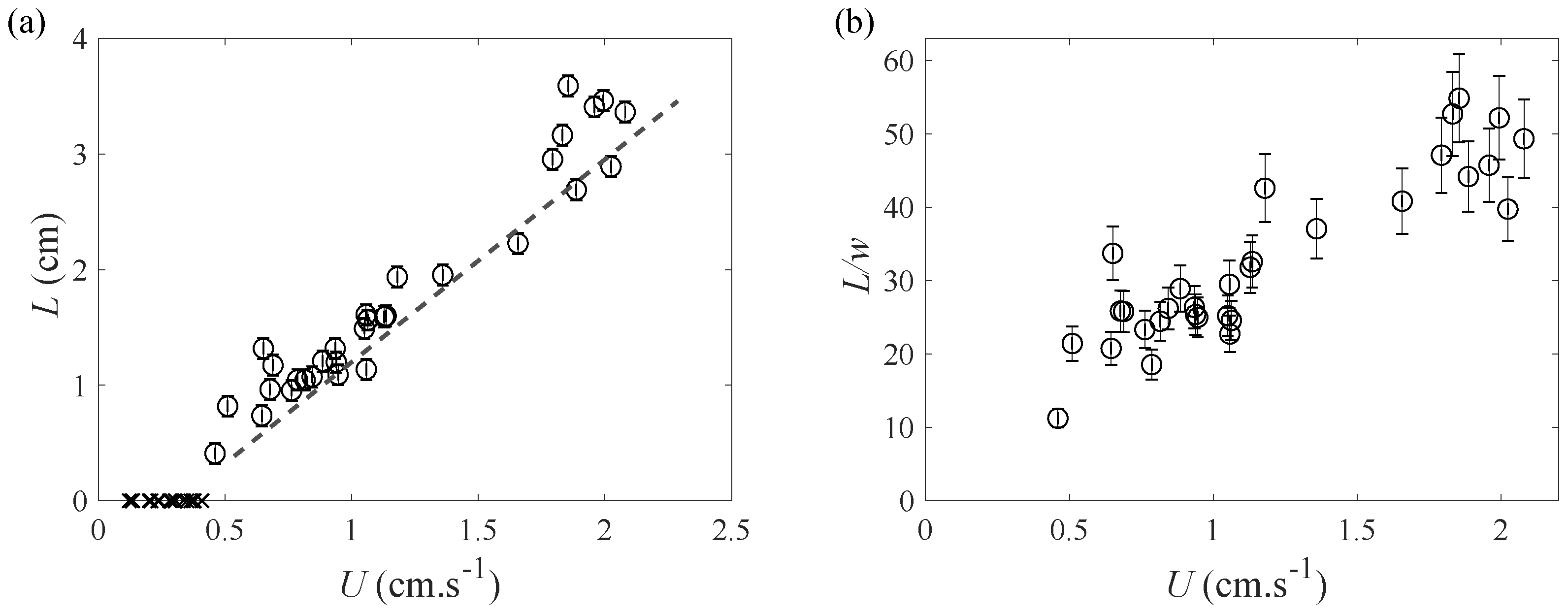
Since we photograph the drop in a terminal condition, we do not observe the initial formation of the tail. As for the volume of the drop, the length L and width w of the tail might change during the rising, since droplets are emitted, but, once again, we did not observe a significant reduction of either the length or the width of the tail over the height of the camera window (12 cm). We measured the length L and the width w once the tail was fully visible in the images. Figure 5a shows the length of the tail as a function of the velocity of the drop U. We observe a breakup of the end of the tail leading to droplets’ emission at a distance going from 0.5 to 3.6 cm from the main drop. This distance (which corresponds to what we called the tail length L) will vary linearly with the velocity U, with a slope of 1.5 s (dashed line, Figure 5a). This shows that the length of the tail depends directly on the velocity of the drop, via the negative wake. The slope corresponds to the time needed for the drop to move a distance L.

Figure 5b shows the tail aspect ratio $L/w$ as a function of the drop velocity U. This aspect ratio is between 10 (for the drop at the transition), up to 50 for the largest drops. This shows that the tail is very long compared to its width, the width being for the smallest tail of about 0.035 cm to 0.075 cm for the biggest one. The fact that the curve increases shows that the tail will grow more rapidly with the velocity U in length L than in width w. We can explain this by the fact that the main driving force for the length of the tail is the strong non-Newtonian behaviour of the fluid, while the width of the tail is limited by the capillary length.

4.2. Emission Period and Wavelength

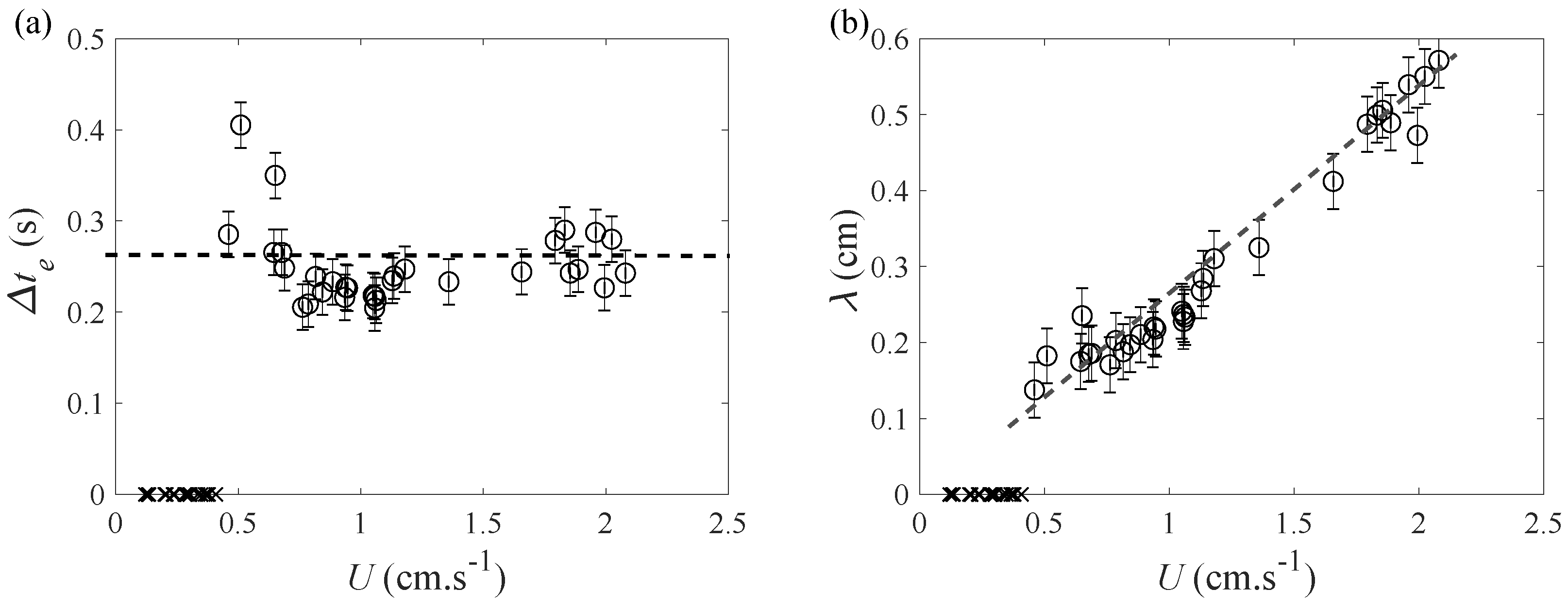
Figure 6a shows the average time $\mathsf{\Delta }{t}_e$ (or emission period) between two droplets emitted, as a function of the velocity of the drop. Except at the critical velocity $V_c$, the period of emission of droplets $\mathsf{\Delta }{t}_e$ is roughly constant and has a value contained between 0.2 and 0.3 s. This results from a competition between the width w of the tail and the velocity U of the drop. For small velocity, the tail is thinner, so it would tend to break more easily, and, at higher velocity, the drainage of the tail is more rapid, which also helps the breakup. At the end, the time between the emission of two droplets emitted will be roughly the same for all velocity.

Figure 6b shows the average distance between two droplets $\lambda$, as a function of the velocity of the drops U. This distance increases importantly with velocity, which is in agreement with the constant emission period $\mathsf{\Delta }{t}_e$: since the tail velocity is the same as the drop velocity U (stationary regime), and the emission time between two drops is almost constant; this implies that the distance between two drops will increase with the velocity of the drop. We have a linear relation between $\lambda$ and U for the drops over the critical volume $V_c$, with a slope of $\mathsf{\Delta }{t}_e\approx$ 0.27 s (dashed line, Figure 6b), which is in accordance with Figure 6a. We can compute the frequency of emission of the droplets, if we assume that the velocity is constant during one run, which gives us $f_e=1/\mathsf{\Delta }{t}_e\approx 3.7$ s⁻¹.

4.3. Droplet Size

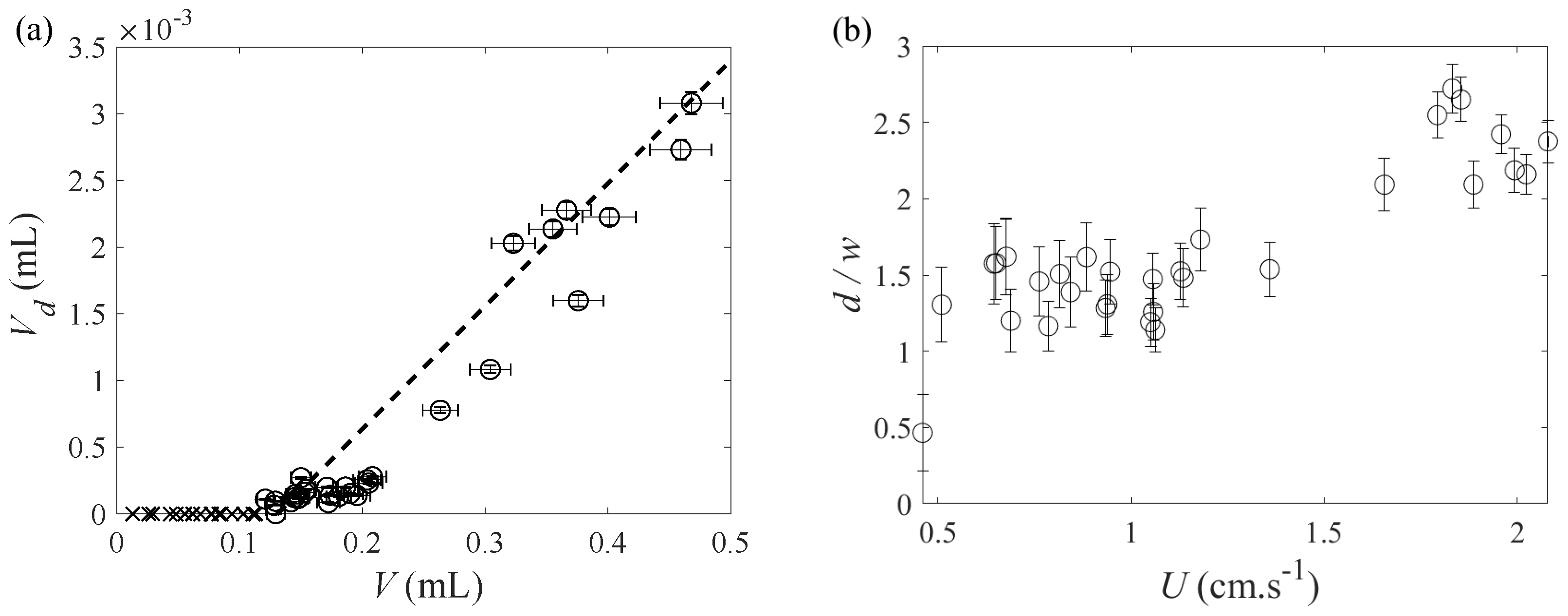
We also analyzed the size of the droplets created behind the main drop. Once again, we observe that the size of the droplets is constant over the course of one experiment (for one given drop volume V). The contrast being better for the droplets than the drop, the uncertainty on the diameter gets to about one pixel, but it is still important in comparison with the droplet diameter. To reduce the error, we measure the diameter for 10 different droplets, which decrease significantly the error, down to an estimated 5 percent. The error bars have been reported on Figure 7. We used the same method to estimate the width of the tail, measuring the width at different heights and then averaging. Figure 7a shows the average volume of the droplets $V_d$ as a function of the volume of the main drop V. The volume of the droplets $V_d$ has been computed assuming that the droplet is a sphere: $V_d=\pi d^3/6$, where d is the diameter of the droplets (see Figure 3e). We observe that the volume of the droplets increases linearly with the volume of the drop. This will be used to calculate the volume loss of the main drop over time (Section 5.2).

Figure 7b shows the normalized droplet diameter $d/w$ as a function of the velocity of the drop U. We observe that this ratio increases with the velocity, and, most of all, its value is always larger than one (except for one point at the transition), which means that the droplets are wider than the tail before it breaks. This can be explained by a simple mass conservation argument. The volume of oil before the break corresponds to the volume of a column of width w and height $\lambda$ (for one wavelength), and also to the volume of one droplet of diameter d. We can write this volume as $V_d=\pi /4\lambda w^2=\pi d^3/6$. Therefore,

$$\frac{d^2}{w^2}=3/2\frac{\lambda }{d}.$$

(1)

Considering that the distance of between two droplets is much bigger than the size of the droplet except at the critical volume (see Figure 3), we have $\lambda /d>1$, and so the diameter of the droplet d will be bigger than the width of the tail w.

5. Discussion

5.1. Tail Appearance and Breakup

We observe that a tail appears behind the drop for a volume larger than the critical one, $V_c=0.13$ mL. This critical volume corresponds to the appearance of a negative wake behind the drop. This negative wake has been already studied in various cases, for bubbles [14,15,16,18,20,21,23], and for drops [11,17,20]. The main difference between the drop and the bubble case is that the interfacial tension between the air and the liquid is larger than that for two liquids. The bubble shape will then remain the same over the course of the experiment, while in the case of a drop, this interface is more deformable, and the tail will be able to grow due to the negative wake [20]. This negative wake will be more important as the velocity U increases, and the width of the tail w will also increase. The tail will then grow to a length L, where it will break up into small droplets. The size of these droplets is controlled by their emission frequency $f_e$, or its corresponding wave length, $\lambda$.

This breakup is similar to the Rayleigh–Plateau instability which arises from capillary effects [24,25]. The temporal evolution of this rupture, which fixes the length of the tail L, is hard to predict, as it takes into account the velocity of the fluid inside the tail. We do not have access to this velocity (it would require Particle Image Velocimetry (PIV) in the oil phase), and it is hard to predict it since it results from the negative wake. The fact that the length L increases with the velocity U is not trivial, but we can assume that the breakup occurs when the oil at the tip of the tail has a zero velocity. This would be in agreement with the negative wake increasing with the velocity of the drop. One way to describe such type of instabilities is to look at the capillary number and capillary length. The capillary number is the ratio between the capillary and the viscous forces: $\mathrm{Ca}=\eta U^{\prime }/\sigma$, where $\sigma$ is the interfacial tension between the two fluids. In this case, $U^{\prime }$ is the speed of the droplets and not the velocity of the drop, but since we are in a stationary regime, we have $U^{\prime }=U$. Since we have a proportionality between the wavelength $\lambda$, and the velocity $U=U^{\prime }$, and the shear-thinning behaviour is small, we have a direct proportionality between the capillary number Ca and the wavelength $\lambda$:

$$\lambda =\mathsf{\Delta }{t}_e{U}^{\prime }=k·\mathrm{Ca},$$

(2)

where $k=\mathsf{\Delta }{t}_e\sigma /\eta$ is a constant coefficient with the dimension of a length. An important difficulty is to determine the interfacial tension $\sigma$ between the two phases. In the literature, the corn oil surface tension is reported to be ${\sigma }_{oil}\approx 33.5$ mN/m [35] and for the polyacrylamide solution ${\sigma }_{PAAM}\approx 75$ mN/m [36]. At the first order, Antonoff’s rule gives the interfacial tension between the two phases $\sigma = |{\sigma }_{PAAM}-{\sigma }_{oil}| \approx 41.5$ mN/m. By considering that $\eta \approx 0.9$ Pa.s, we obtain that $k\approx 1.24$ cm. The capillary length can be defined as $l_c=\sqrt{\sigma /\mathsf{\Delta }\rho g}\approx 1.29$ cm, where $\mathsf{\Delta }\rho$ is the density difference between the two fluids, and g is the gravitational acceleration. Therefore, $k\approx l_c$, which is consistent with the assumption that, indeed, the breakup of the tail results from capillary instability. This scaling relies on important assumptions, notably on the value of the interfacial tension. In addition, it does not take into account the viscoelastic properties of the surrounding fluid. Nevertheless, these scaling arguments indicate that indeed the tail is fragmenting mainly as a result of capillary instability and the viscoelastic effects are secondary.

5.2. Volume Loss

It is important to evaluate the role of volume change for the main drop, resulting from the droplets emitted at the tail. In all cases, we assumed that the drop volume V was constant. This assumption is supported by two facts. First, in Figure 4a, the bubble rises at a constant velocity, which would not have been the case if the volume had varied significantly. Secondly, Figure 7a show that the volume of the droplets $V_d$ remains smaller than 0.65 percent of the main drop volume, for the largest drops. In this case, only 20 droplets are emitted over the experiment, which makes (in the worst case scenario) a volume loss around 13 percent of the initial drop volume.

A simple model is proposed to predict the volume of the droplets in an infinitely long liquid column. First, by using the linear regression in Figure 7a, we can predict the volume of a droplet knowing the volume of the main drop. Then, assuming that the emission frequency of droplets is constant $f_e=3.7$ s⁻¹ (Figure 6a), we can write the following differential equation for the volume change:

$$\frac{\mathrm{d}V}{\mathrm{d}t}=-f_e{V}_d=-f_e(\alpha ·V+\beta ),$$

(3)

where $\alpha =9.2\times {10}^{-3}$ and $\beta =-1.2\times {10}^{-3}$ mL are the slope and intercept of the dashed line in Figure 7a. Integrating, we obtain

$$V\left(t\right)=V_0\exp (-f_e·\alpha ·t)+\frac{\beta }{\alpha }(\exp (-f_e·\alpha ·t)-1),$$

(4)

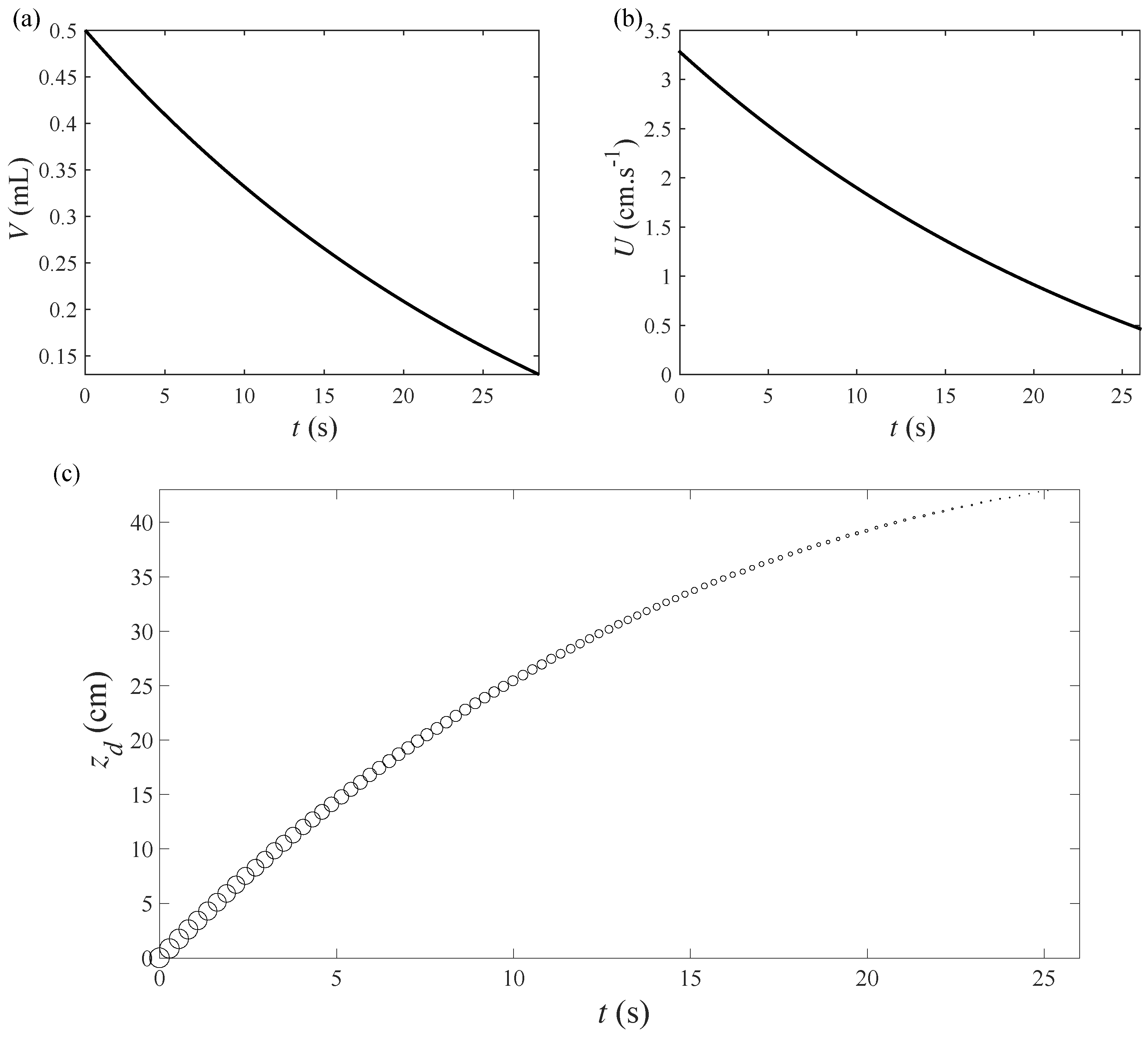
where $V_0$ is the initial drop volume (taken to be 0.5 mL). This expression, if used carelessly, will predict a negative volume value for long times; however, one must consider that the droplets will no longer be emitted once the volume $V\left(t\right)$ reaches the critical volume ($V_c=0.13$ mL). The drop will then rise with a constant volume $V_c$ and a constant velocity $U_c\approx 0.46$ cm·s⁻¹. Figure 8a shows the volume evolution $V\left(t\right)$ as a function of time t. The critical volume $V_c$ is reached at a time $t_c=26$ s.

We can use a linear regression between the volume and the velocity over the critical volume in Figure 4b which gives $U\left(t\right)=7.6V\left(t\right)-0.52$. Figure 8b shows the velocity of the drop U, as a function of time t, the velocity decreases from 3.3 cm·s⁻¹ to $U_c=0.46$ cm·s⁻¹. This is clearly only a first order approximation, since the relation between the volume and velocity is most likely nonlinear. It allows us to continue the integration. We can then compute the position $z\left(t\right)$ of the drop as a function of time as:

$$z\left(t\right)={\int }_0^{t}U\mathrm{d}{t}^{\prime }={\int }_0^t(7.6V\left(t\right)-0.52)\mathrm{d}{t}^{\prime }.$$

(5)

For simplicity, we will not write down this integral (it implies exponential integrals). Figure 8c shows the position of the droplets emitted $z_d$, as a function of time t. The droplets are emitted every $\mathsf{\Delta }{t}_e=0.27$ s, and the marker size is proportional to the volume of the droplets. The drop will reach its critical volume at a position $z_c=43.4$ cm, and then will rise at its constant velocity, without emitting new droplets. The volume of the droplets emitted will vary from $V_d=0.0034$ mL at the beginning, and will tend to 0 when we approach the critical volume. We must emphasize that the calculation above is only valid for the two-fluid combination considered here. However, the same general behaviour is expected for a Newtonian/non-Newtonian combination. Clearly, more experiments are needed to extend the parametric range of validity. This simple model gives us an order of magnitude of what should be expected in terms of time $t_c$ and height $z_c$ for the bubble to reach its critical volume $V_c$. This is in agreement with what was shown before: $t_c$ is much bigger than the time of our experiment (10 s), and $z_c$ is also much bigger than the 12 cm where we observed the rise, so the model holds some consistency. This simple model could lead to some applications. For instance, we could imagine a device where one would like to encapsulate oil droplets (containing another substance to analyze or to use as a reactant for example) with droplets varying in size. With this simple two-fluid configuration, and by choosing well both fluids (which would require more experiments and more general understanding), one could construct such device, which would be very easy to use since the only input would be the volume of the main drop. Since the emitted droplets would be small, their rising velocity would be small too. Hence, their capture would be relatively simple. Additionally, one could use a surrounding yield-stress viscoelastic fluid, so that the encapsulated droplets would be completely trapped and then easily manipulated.

6. Conclusions and Perspectives

In this article, we investigated the instability occurring at the tail of a Newtonian drop rising in a viscoelastic fluid. We observe that this leads to the formation of small droplets, which are controlled in size by the velocity of the drop, which in turn depends on its volume. It is interesting to note that such behaviour (cusp and tail formation with fragmentation) had not been discussed previously in this combined manner. In this article, we use the results of a very particular case where the rising drop presents a velocity discontinuity and a negative wake (corn oil in a polyacrylamide solution), so the physical properties of the fluids are fixed. We described the appearance of a tail resulting from the negative wake over a critical volume and its breakup due to capillary forces. This limits our results to the ranges of Reynolds and Deborah number we used. To provide a more general understanding, more experiments are needed, by changing both fluids. A number of open questions remain, notably on the role of the viscosity ratio between both fluids, the interfacial tension, the quantitative role of the surrounding fluid elasticity, for both the tail formation and the breakup, as well as the role of elongational rheology (since we are dealing with polymer solutions). An exhaustive study would require a very important number of experiments, since changing fluids will influence all the properties at once (density, viscosity, elasticity, critical volume, etc.). We plan to pursue such experiments in the future. Finally, we proposed a simple model, based on the volume of the emitted droplets, that could have some application to encapsulate droplets with varying size, with just one input: the volume of the main drop.

References

- Wu, L.; Chen, P.; Dong, Y.; Feng, X.; Liu, B.F. Encapsulation of single cells on a microfluidic device integrating droplet generation with fluorescence-activated droplet sorting. Biomed. Microdevices 2013, 15, 553–560. [Google Scholar] [CrossRef] [PubMed]
- Teh, S.Y.; Lin, R.; Hung, L.H.; Lee, A.P. Droplet microfluidics. Lab Chip 2008, 8, 198–220. [Google Scholar] [CrossRef] [PubMed]
- Theberge, A.B.; Courtois, F.; Schaerli, Y.; Fischlechner, M.; Abell, C.; Hollfelder, F.; Huck Wilhelm, T.S. Microdroplets in Microfluidics: An Evolving Platform for Discoveries in Chemistry and Biology. Angew. Chem. Int. Ed. 2013, 49, 5846–5868. [Google Scholar] [CrossRef] [PubMed]
- Mark, D.; Haeberle, S.; Roth, G.; Von Stetten, F.; Zengerle, R.L. Microfluidic Lab-on-a-Chip Platforms: Requirements, Characteristics and Applications. In Microfluidics Based Microsystems; Kakaç, S., Kosoy, B., Li, D., Pramuanjaroenkij, A., Eds.; Springer: Dordrecht, The Netherlands, 2010; pp. 305–376. ISBN 978-90-481-9029-4. [Google Scholar]
- Garstecki, P.; Fuerstman, M.J.; Stone, H.A.; Whitesides, G.M. Formation of droplets and bubbles in a microfluidic T-junction—Scaling and mechanism of break-up. Lab Chip 2006, 6, 437–446. [Google Scholar] [CrossRef] [PubMed]
- De Menech, M.; Garstecki, P.; Jousse, F.; Stone, H. Transition from squeezing to dripping in a microfluidic T-shaped junction. J. Fluid Mech. 2008, 595, 141–161. [Google Scholar] [CrossRef]
- Arigo, M.T.; McKinley, G.H. An experimental investigation of negative wakes behind spheres settling in a shear-thinning viscoelastic fluid. Rheol. Acta 1998, 37, 307–327. [Google Scholar] [CrossRef]
- Bisgaard, C.; Hassager, O. An experimental investigation of velocity fields around spheres and bubbles moving in non-Newtonian liquids. Rheol. Acta 1982, 21, 537–539. [Google Scholar] [CrossRef]
- Broadbent, J.; Mena, B. Slow flow of an elastico-viscous fluid past cylinders and spheres. Chem. Eng. J. 1974, 8, 11–19. [Google Scholar] [CrossRef]
- Caswell, B.; Manero, O.; Mena, B. Recent developments on the slow viscoelastic flow past spheres and bubbles. Rheol. Rev 2004, 197–223. [Google Scholar]
- Chhabra, R.P. Bubbles, Drops and Particles in Non-Newtonian Fluids; CRC Press: Boca Raton, FL, USA, 1993. [Google Scholar]
- Manero, O.; Mena, B. On the slow flow of viscoelastic fluids past a circular cylinder. J. Non-Newton. Fluid Mech. 1981, 9, 379–387. [Google Scholar] [CrossRef]
- Mena, B.; Manero, O.; Leal, L.G. The influence of rheological properties on the slow flow past spheres. J. Non-Newton. Fluid Mech. 1987, 26, 247–275. [Google Scholar] [CrossRef]
- Herrera-Velarde, J.R.; Zenit, R.; Chehata, D.; Mena, B. The flow of non-Newtonian fluids around bubbles and its connection to the jump discontinuity. J. Non-Newton. Fluid Mech. 2003, 111, 199–209. [Google Scholar] [CrossRef]
- Rodrigue, D.; De Kee, D. Bubble velocity jump discontinuity in polyacrylamide solutions: A photographic study. Rheol. Acta 1998, 37, 307–327. [Google Scholar] [CrossRef]
- Rodrigue, D.; De Kee, D.; Chan Man Fong, C. Bubble velocities: further developments on the jump discontinuity. J. Non-Newton. Fluid Mech. 1998, 79, 45–55. [Google Scholar] [CrossRef]
- Zenit, R.; Feng, J.J. Hydrodynamic Interactions Among Bubbles, Drops, and Particles in Non-Newtonian Liquids. Annu. Rev. Fluid Mech. 2018, 50, 505–534. [Google Scholar] [CrossRef]
- Astarita, G.; Apuzzo, G. Motion of gas bubbles in non-Newtonian liquids. AIChE J. 1965, 11, 815–820. [Google Scholar] [CrossRef]
- Pilz, C.; Brenn, G. On the critical bubble volume at the rise velocity jump discontinuity in viscoelastic liquids. J. Non-Newton. Fluid Mech. 2007, 145, 124–138. [Google Scholar] [CrossRef]
- Ortiz, S.L.; Lee, J.S.; Figueroa-Espinoza, B.; Mena, B. An experimental note on the deformation and breakup of viscoelastic droplets rising in non-Newtonian fluids. Rheol. Acta 2016, 55, 879–887. [Google Scholar] [CrossRef]
- Soto, E.; Goujon, C.; Zenit, R.; Manero, O. A study of velocity discontinuity for single air bubbles rising in an associative polymer. Phys. Fluids 2006, 18, 121510. [Google Scholar] [CrossRef]
- Fraggedakis, D.; Pavlidis, M.; Dimakopoulos, Y.; Tsamopoulos, J. On the velocity discontinuity at a critical volume of a bubble rising in a viscoelastic fluid. J. Fluid Mech. 2016, 789, 310–346. [Google Scholar] [CrossRef]
- Hassager, O. Negative wake behind bubbles in non-Newtonian liquids. Nature 1979, 279, 402–403. [Google Scholar] [CrossRef] [PubMed]
- Lister, J.R.; Stone, H.A. Capillary breakup of a viscous thread surrounded by another viscous fluid. Phys. Fluids 1998, 10, 2758–2764. [Google Scholar] [CrossRef]
- De Gennes, P.G.; Brochard-Wyart, F.; Quéré, D. Capillary and Wetting Phenomena—Drops, Bubbles, Pearls, Waves; Alex, R., Translator; Springer: Berlin/Heidelberg, Germany, 2002. [Google Scholar]
- Deblais, A.; Velikov, K.P.; Bonn, D. Pearling instabilities of a viscoelastic thread. Phys. Rev. Lett. 2018, 120, 194501. [Google Scholar] [CrossRef] [PubMed]
- Clasen, C.; Eggers, J.; Fontelos, M.A.; Li, J.; McKinley, G. The beads-on-string structure of viscoelastic threads. J. Fluid Mech. 2006, 556, 283–308. [Google Scholar] [CrossRef]
- Skelland, A.H.P.; Raval, V.K. Drop size in power law non-Newtonian systems. Can. J. Chem. Eng. 1972, 50, 41–44. [Google Scholar] [CrossRef]
- Kitamura, Y.; Takahashi, T. Breakup of jets in power law non-Newtonian–Newtonian liquid systems. Can. J. Chem. Eng. 1982, 60, 732–737. [Google Scholar] [CrossRef]
- Teng, H.; Kinoshita, C.M.; Masutani, S.M. Prediction of droplet size from the breakup of cylindrical liquid jets. Int. J. Multiph. Flow 1995, 21, 129–136. [Google Scholar] [CrossRef]
- Barnes, H.A.; Hutton, J.F.; Walters, K. An Introduction to Rheology; Elsevier: New York, NY, USA, 1989. [Google Scholar]
- Ghannam, M.T.; Esmail, M.N. Rheological properties of aqueous polyacrylamide solutions. J. Appl. Polym. Sci. 1998, 69, 1587–1597. [Google Scholar] [CrossRef]
- Palacios-Morales, C.; Zenit, R. The formation of vortex rings in shear-thinning liquids. J. Non-Newton. Fluid Mech. 2013, 194, 1–13. [Google Scholar] [CrossRef]
- Mendoza-Fuentes, A.J.; Manero, O.; Zenit, R. Evaluation of drag correction factor for spheres settling in associative polymers. Rheol. Acta 2010, 49, 979–984. [Google Scholar] [CrossRef]
- Esteban, B.; Riba, J.-R.; Baquero, G.; Puig, R.; Rius, A. Characterization of the surface tension of vegetable oils to be used as fuel in diesel engines. Fuel 2012, 102, 231–238. [Google Scholar] [CrossRef]
- Hu, R.Y.Z.; Wang, A.T.A.; Hartnett, J.P. Surface tension measurement of aqueous polymer solutions. Exp. Therm. Fluid Sci. 1991, 4, 723–729. [Google Scholar] [CrossRef]
Figure 1.
Scheme of the experimental set-up. In a vertical glass column with a square base of 6 cm side width and a height of 60 cm, we place a non-Newtonian fluid. An oil drop is injected at the bottom of the column using a plastic syringe. The images are recorded using a fast speed camera (200 fps), and the set-up is backlit using a LED panel. Behind the drop, we observe formation of droplets.
Figure 2.
(a) table compiling the properties of the two fluids used. Since the oil drop has a lower density and a Newtonian behaviour, it will rise in the surrounding fluid consisting of a water-polyacrylamide solution, which is denser and has shear-thinning and viscoelastic properties; (b) measured viscosity as a function of the shear-rate for the two fluids used. The diamonds represent the oil drop (Newtonian), the squares the polyacrylamide solution (Shear-thinning). is the shear-rate range in our experiment and the dashed line corresponds to the power-law fit; (c) elastic modulus G’ (full squares) and viscous modulus G’’ (empty squares) as a function of the oscillation frequency for the polyacrylamide solution. A viscoelastic behaviour is clearly observed. The relaxation frequency , is estimated when the two moduli are the closest. In (b,c), the measurements are performed both increasing and decreasing the shear-rate/oscillation frequency.
Figure 3.
Different regimes observed: (a) before the tail appears; (b) at the critical volume mL, where the tail appearance is. We can see very small droplets appearing behind the tail of the main drop; (c–e) instability for different volumes. We can observe that the tail length L, the width of the tail w, the distance between two droplets and the droplets diameter d increases with the volume. Those are defined in (e) and this will be discussed in detail in Section 4.
Figure 4.
(a) position of the front of the drop as a function of time. This example corresponds to Figure 3e. We observe that the rising velocity U stays constant over the 12 cm experiment height; (b) rising velocity U of the drops, as a function of the volume V. We observe a small velocity jump at the moment of the tail appearance for a critical volume mL and a critical velocity cm·s−1.
Figure 5.
(a) tail length L as a function of the velocity of the drop U. We see clearly a critical velocity where the tails appears (corresponding to a critical volume ). The tail length grows linearly with the speed of the drop (dashed line); (b) tail aspect ratio as a function of the drop velocity V. The tail has a very elongated shape.
Figure 6.
(a) period of emission of the droplets (average time between two droplets appearance), as a function of the drop velocity U. Except close to the critical volume, this period seems roughly constant (dashed line, s), which corresponds at a frequency of emission of 3.7 Hz; (b) wavelength (average distance between two droplets), as a function of the drop velocity U. The dashed line represents the linear adjustment.
Figure 7.
(a) mean volume of the droplets as a function of the volume of the drop V. We observe an important increase which is coherent with Figure 3. The dashed line represents the linear regression, which will be used in Section 5; (b) droplet diameter d divided by the tail width w as a function of the drop velocity U. We observe that, except for the critical case, the diameter of the droplets is always bigger than the tail width.
Figure 8.
(a) evolution of the volume V as a function of time t. The critical volume mL is reached after a time s; (b) velocity of the droplet U as a function of time t; (c) velocity of the droplet U as a function of time t; (c) position of the droplets as a function of time t. The size of the markers represents the volume of each droplet.
© 2018 by the authors. Licensee MDPI, Basel, Switzerland. This article is an open access article distributed under the terms and conditions of the Creative Commons Attribution (CC BY) license (http://creativecommons.org/licenses/by/4.0/).
Share and Cite
MDPI and ACS Style
Poryles, R.; Zenit, R. Encapsulation of Droplets Using Cusp Formation behind a Drop Rising in a Non-Newtonian Fluid. Fluids 2018, 3, 54. https://doi.org/10.3390/fluids3030054
AMA Style
Poryles R, Zenit R. Encapsulation of Droplets Using Cusp Formation behind a Drop Rising in a Non-Newtonian Fluid. Fluids. 2018; 3(3):54. https://doi.org/10.3390/fluids3030054
Chicago/Turabian StylePoryles, Raphaël, and Roberto Zenit. 2018. "Encapsulation of Droplets Using Cusp Formation behind a Drop Rising in a Non-Newtonian Fluid" Fluids 3, no. 3: 54. https://doi.org/10.3390/fluids3030054