Climate Change Impacts on Water Use in Horticulture

Abstract

The evidence for anthropogenic global climate change is strong, and the projected climate changes could greatly impact horticultural production. For horticulture, two of the biggest concerns are related to the scarcity of water for crop production and the potential for increased evapotranspiration (ET). While ET is known to increase with air temperature, it is also known to decrease with increasing humidity and atmospheric CO₂ concentration. Considering all of these factors and a plausible climate projection, this paper demonstrates that ET may increase or decrease depending on the magnitude of atmospheric changes including wind speed. On the other hand, the evidence is still strong that water resources will become less reliable in many regions where horticultural crops are grown.

1. Introduction

Most scientists agree that global climate change is occurring at an alarming rate and that these changes are likely to impact water use in horticulture, agronomy, and natural ecosystems. In some locations, climate change can potentially increase agricultural production, but it is generally believed that widespread detrimental impacts on agricultural production are more likely in much of the world. Currently, the global climate change trend is for increasing air temperature, mainly at night and during winter, and more near the poles than in lower latitudes. Because of global warming, energy storage in water has increased dramatically (much more than in the air), and higher water temperatures has led to rising sea level due to water expansion and additional heat storage mainly in the oceans. In addition, increasing air and water temperature enhances evaporation, and higher air temperature increases the saturation water vapor pressure, i.e., the amount of water vapor that is held in the air at saturation. These atmospheric changes can impact plant growth, production, and water usage, and this chapter presents ideas on the possible impact of higher temperature, humidity, and CO₂ concentration on the evapotranspiration (ET) of horticultural crops.

At this time, the main cause for global climate change is the increasing concentration of CO₂. According to the “Keeling curve,” the CO₂ concentration recorded at the Mauna Loa Observatory in Hawaii (USA) increased from about 315 to 395 ppm from 1958 to 2013, and recently passed 400 ppm. This increase has serious implications for global climate change and its impact on nature and horticulture.

The greenhouse gases (GHGs) that contribute most to global climate change from the worst to least worse are as follows: (1) H₂O—water vapor; (2) CO₂—carbon dioxide; (3) NH₄—methane; (4) N₂O—nitrous oxide; (5) O₃—ozone. While H₂O is actually a more effective GHG than CO₂, the atmospheric concentration is spatially and temporally variable and it is not increasing rapidly at this time. However, as the oceans warm, higher concentrations of atmospheric H₂O are likely, and the higher levels can greatly contribute to warming. Carbon dioxide is a less effective GHG than H₂O, but the more evenly distributed global concentration is increasing steadily, and it is currently the GHG causing the most rapid global temperature rise. Methane is a concern for the future because large amounts of methane are stored in the ocean and in permafrost. Scientists believe that thawing the permafrost and warming the oceans might release this stored NH₄ and cause a rapid temperature increase. Nitrous oxide is used as an aerosol propellant, anesthetic, and an oxidizer in rockets and engine fuel. Ozone is not evenly distributed over the Earth’s surface, but man-made O₃ does contribute to atmospheric warming in urban areas.

GHGs mostly reside in the troposphere, i.e., the lowest level of the atmosphere, where they intercept long waveband radiation (LWR) and raise atmospheric temperatures. The stratosphere, which is a stable layer of air above the troposphere, has considerably less greenhouse gas than the troposphere, and, interestingly, this upper atmospheric layer is cooling. If the global warming were caused by increasing solar output or reduced reflection of solar radiation, the troposphere and stratosphere would both likely have increasing temperatures. Consequently, the simultaneous troposphere warming and stratosphere cooling is a good indicator that the warming is caused by anthropogenic increases in GHG additions (mostly CO₂) to the atmosphere. The melting of polar ice packs is a strong indication of global warming, and it will likely compound the warming because less solar radiation will be reflected back to space as the ice melts.

Climate change is likely to cause sea level rise and damage plant and animal life in the oceans and on land. Of course, changes in temperature and humidity could also lead to changes in general circulation of the atmosphere, greater frequency of storms and floods, and changes in the length and severity of drought. In general, climate scientists are projecting more frequent and severe storms and drought due to changes in atmospheric circulation [1]. In terms of horticulture, the authors of [2] and [3] discuss several potential effects of climate change on horticulture. In some cases, increasing CO₂, temperature, humidity, and other greenhouse gases might be beneficial in regions where crop production is limited by cold temperatures due to (1) lower potential for frost damage, (2) faster growth, and (3) lengthened growing seasons. In addition, there is some benefit coming from CO₂ fertilization, which can enhance photosynthesis. On the other hand, climate change could negatively impact agriculture in regions where climate conditions are currently good for production. For example, climate change might (1) decrease chilling and inhibit bloom and fruit set in horticultural crops, (2) lead to high temperature and wind during bloom or ripening that could negatively impact fruit set or fruit quality, (3) increase ET rates that could lead to water deficits, and (4) increase problems with heat stress.

Some possible climate change impacts on agriculture include (1) droughts, (2) floods, (3) faster phenological development, (4) inadequate chilling requirements, (5) pollination affected by rainfall and other extreme events, (6) frost and chill damage, (7) the spread of new insects and diseases, and (8) lower or higher yield and quality due to warming and water relations during summer [2,3]. One example of warming impacts is decreased winter chilling, which leads to bad pollination, staggered bloom, reduced fruit set, and poor fruit quality. In low chill years, apricots and cherries can drop flower buds or not produce a crop when chilling is inadequate.

In some regions, winter fog is an important factor in achieving adequate chilling for some crops. Rainfall during bloom can inhibit bee pollination, and precipitation around harvest time can increase fruit and nut diseases, cause fruit cracking, and destroy a crop. In deciduous orchards, late spring and summer rainfall has a negative effect on fruit and nut quality and production. Clearly, there are a multitude of climate factors that can change to wreak havoc on the production of horticultural crops. For example, climate scientists are projecting more bimodal precipitation in California, with more precipitation in the spring and fall and less in the winter. However, California depends on water storage in the mountain snowpack, and higher snow lines in the mountains, especially in the north where the mountains are shorter, will have less snowpack storage and will result in less water delivery to agricultural land in the summer [4]. Snowpack storage will affect the collection and distribution of irrigation water, but precipitation timing will also affect rainfall damage to crops in the spring and fall as well as changes in fog formation due to winters with higher temperatures and less rainfall.

While all of the aforementioned changes and impacts are important to consider, it is difficult to project changes in general circulation, storms, and drought with a high degree of accuracy in any particular region on Earth. However, the general impact of widespread higher temperatures, humidity, and increased CO₂ on factors affecting crop production is possible. Following a short discussion on how rising CO₂ concentrations cause global warming, this paper will present some ideas on the possible impact of higher temperature, humidity, and CO₂ on ET.

2. Increasing CO₂ and Global Warming

The impact of atmosphere CO₂ concentration on the greenhouse effect and the Earth’s surface temperature was first described by Svante August Arrhenius [5]. Although climate science has advanced considerably since Arrhenius first made his estimates of increasing CO₂ concentration, its impact on global temperature is still quite accurate. Equations (1)–(3) are modified versions of the original equations from [5]. Equation (1) provides an estimate of Earth’s emission temperature (T_e), which is the mean surface temperature it would have if there were no atmosphere:

$$T_e={\left[\frac{\pi r^2\left(1-{\alpha }_p\right)R_{sc}}{4\pi r^2\sigma }\right]}^{\frac{1}{4}}={\left[\frac{\left(1-{\alpha }_p\right)R_{sc}}{4\sigma }\right]}^{\frac{1}{4}}\approx 255 \mathrm{K}$$

(1)

where R_SC = 1631 W·m⁻² is the solar constant, α_p ≈ 0.30 is the albedo (reflection of solar radiation from the surface), r ≈ 6371 × 10³ m is the mean Earth radius, π = 3.1415927, and σ = 5.67 × 10⁻⁸ J·s⁻¹·m⁻²·K⁻⁴ is the Stefan–Boltzmann constant. Based on Equation (1), if we had no atmosphere, the Earth’s mean surface temperature would be approximately T_e = 255 K = −18 °C.

Adding gases to the atmosphere has a minimal impact on the surface solar radiation balance, but greenhouse gases in the atmosphere are known to intercept upward and downward fluxes of LWR, which raises the atmospheric temperature. Assuming a single layer atmosphere that is opaque to LWR, it can be shown that Equation (2) provides an estimate of the maximum Earth surface temperature (T_s) assuming that all of the LWR is absorbed by the atmosphere.

$$T_s=2^{0.25}·T_e\approx 1.19·T_e=303 \mathrm{K}.$$

(2)

Thus, if the GHG in the atmosphere was 100% efficient at intercepting LWR, the maximum surface temperature would be T_s = 303 K = 30 °C. Therefore, with current solar radiation, short waveband radiation reflection, and GHGs, the actual surface temperature of Earth falls somewhere between −18 °C and 30 °C.

Assuming a single layer leaky atmosphere, which allows for some loss of LWR back to space, it can be shown that Equation (3) provides an estimate of the Earth surface temperature (T_s) as a function of T_e and the fraction of upward LWR absorbed by the atmosphere (ϵ). Until the GHG concentration began to increase, about 78% of the LWR was absorbed by GHGs in the atmosphere. Therefore, using Equation (3) and ϵ = 0.78 shows that GHG increased the Earth’s surface temperature from −18 °C to 15 °C (288 K).

$$T_s={\left(\frac{2}{2-ϵ}\right)}^{\frac{1}{4}}{T}_e={\left(\frac{2}{2-ϵ}\right)}^{\frac{1}{4}}\left(255\right)\approx 288\mathrm{K}.$$

(3)

Equation (3) illustrates that T_s is affected only by T_e and ϵ, and Equation (1) shows that T_e is affected only by the amount of incoming and reflected solar radiation. Thus, only the incoming and reflected short waveband radiation and GHG concentration determine the Earth’s global surface temperature. Since 1958, changes in R_SC and α_p were insignificant; however, the anthropogenic releases of CO₂ and other GHGs led to a rise of more than 80 ppm in atmospheric CO₂ concentration. The rising CO₂ concentration increased ϵ and it is the most likely cause for most of the corresponding 1 °C increase in global temperature [6]. Based on [1], considerably more global warming is projected as CO₂ levels continue to rise. While global temperature is rising, other climate factors, e.g., humidity, precipitation, wind speed, cloudiness, and precipitation, are also changing, and the assessment of climate change impact on weather and horticultural crops should consider all factors.

3. Impact on Evapotranspiration

Climate change is likely to increase temperature, humidity, and stomatal resistance of plants, and all of those parameters affect ET. It is common for people to associate higher ET with higher temperature, because evaporation rates do increase with higher temperature. However, evaporation is a physical process, whereas ET is both physical and biological. Increasing temperature will affect ET, but radiation, humidity, wind, and CO₂ concentration also affect ET. All of these factors are needed to properly assess the impact of climate change on plant water usage.

4. Estimating Crop Evapotranspiration

For many decades, scientists, engineers, and irrigation managers have used ET and the water balance method to determine agricultural and urban water demand for water resource planning and delivery and for on-farm and urban irrigation management. Because ET is affected by soil, plant, and atmospheric factors, spatial ET variation is common on different scales. In some climates, one can estimate ET using weather data of large areas, e.g., 50–100 km, but in other locations, microclimates can limit weather-based estimates of ET to small areas, e.g., less than 5 km. In general, the most common practice is to estimate “potential” or “energy-limited” crop evapotranspiration (ET_c) as the product of reference evapotranspiration (ET_ref) and a crop coefficient (K_c). Reference evapotranspiration is the energy-limited ET rate from a broad expanse of a well-watered vegetated surface, e.g., grass or alfalfa.

There are several methods to determine ET_ref, but the most common is to monitor weather over a large grass surface and use an equation to estimate the water use for a selected reference surface. Recently, the authors of [7,8] recommended fixed coefficients to estimate the canopy and aerodynamic resistances as inputs to the Penman–Monteith equation [9] to estimate ET_ref for 0.12-meter-tall and 0.50-meter-tall vegetated surfaces and assigned the symbol ET_o for the short canopy and ET_r for the tall canopy. The equations were called “standardized reference evapotranspiration” because the procedures to compute the ET_o and ET_r were standardized. Strictly speaking, the ET_o and ET_r equations provide estimates of ET from a virtual surface with input coefficients to estimate the appropriate canopy and aerodynamic resistances. However, in practice, the ET_o and ET_r approximate the ET of 0.12-meter-tall cool-season grass and 0.50-meter-tall alfalfa, respectively. Once the ET_ref is known, the ET_c is estimated as either ET_c = ET_o × K_c or ET_c = ET_r × K_cr, where K_cr is specific to ET_r. Because ET_o is more widely used than ET_r, the remaining discussion will only use the ET_o method. Crop coefficients are generally determined as K_c = ET_c/ET_o by calculating the K_c ratio using measured daily ET_c and ET_o from weather data. Global climate change could affect either the ET_o or the K_c, so it is important to assess the impact of climate change on both factors.

5. Reference Evapotranspiration

To assess the possible impact of climate change on ET_o, Snyder et al. [10] used the standardized reference evapotranspiration (ET_o) equation for short canopies [7,8] that uses daily radiation, temperature, humidity, wind speed, and canopy resistance data to calculate ET_o. The following version of the ET_o equation [11] was used for the analysis:

$$E{T}_o=\frac{0.408∆\left(R_n-G\right)+\frac{900\gamma \left(e_s-e_a\right)u_2}{T+273}}{∆+\gamma \left(1+0.34u_2\right)} \left(\mathrm{mm}·{\mathrm{d}}^{-1}\right).$$

(4)

In Equation (4), ∆ (kPa·K⁻¹) is the slope of the saturation vapor pressure curve at the mean daily air temperature, R_n (MJ·m⁻²·d⁻¹) is the net radiation over well-watered grass, G (MJ·m⁻²·d⁻¹) is the soil heat flux density, γ (kPa·K⁻¹) is the psychrometric constant, T (°C) is the mean daily air temperature at a 1.5–2.0 m height, u₂ (m·s⁻¹) is the wind speed measured at 2 m above the ground, and e_s and e_a (kPa) are the saturation and actual vapor pressures of the air measured at a 1.5 m height. Information on how to compute R_n, G, ∆, etc. is provided in [7].

The aerodynamic resistance to sensible and latent heat transfer (r_a) occurs indirectly in two locations in Equation (4). The 0.34 in the denominator comes from the following:

$$\frac{r_c}{r_a}=\frac{70}{208/u_2}\approx 0.34u_2.$$

(5)

In Equation (4), the right-hand side of the numerator could be written as

$$\frac{900\gamma \left(e_s-e_a\right)u_2}{T+273}=\frac{187200\left[\gamma \left(e_s-e_a\right)/\left(T+273\right)\right]}{208/u_2}=\frac{187200\left[\gamma \left(e_s-e_a\right)/\left(T+273\right)\right]}{r_a}.$$

(6)

Therefore, the 208 coefficient is also included in the numerator of Equation (4) (within the 900). The r_c = 70 s·m⁻¹ was estimated from the typical stomatal resistance r_s = 100 s·m⁻¹ (corresponding to stomatal conductance g_s = 0.010 m·s⁻¹ = 10 mm·s⁻¹) for the actively transpiring C₃ grass leaf surface, which was estimated as half of the LAI = 2.88. Therefore, the canopy resistance for 0.12-meter-tall C₃ species grass r_c was calculated as

$$r_c=\frac{r_s}{0.5·LAI}=\frac{100 \mathrm{s}·{\mathrm{m}}^{-1} }{0.5\times 2.88}=69\approx 70 \mathrm{s}·{\mathrm{m}}^{-1}.$$

(7)

Long et al. [12] studied the effect of CO₂ concentration on stomatal conductance of C₃ species plants, and the relationships they reported were used to estimate the impact of increasing CO₂ concentration on canopy resistance of the standardized reference surface. Assuming that the r_c ≈ 70 s·m⁻¹ applies to a 2004 CO₂ concentration of about 372 ppm, estimating a new r_c value for higher CO₂ concentration provides a method to estimate possible impacts of higher CO₂ on ET_o.

Based on eight climate models, the mean air temperature projection for California is about 2.2 °C by 2050 and 4.0 °C by 2100 [13]. The global CO₂ concentration is projected to reach about 550 ppm by 2050 and more than 700 ppm by 2100 [14]. Long et al. [12] reported that stomatal conductance for many C₃ species plants decreased by about 20% when the CO₂ concentration was increased from 372 to about 550 ppm from about 200 independent measurements. Assuming this is true for the stomatal conductance of 0.12-meter-tall C₃ species grass with a stomatal resistance of 100 s·m⁻¹, the stomatal conductance for C₃ grass should decrease from about 10 mm·s⁻¹ to 8 mm·s⁻¹, which corresponds to r_s = 125 s·m⁻¹. Using the same approach used to calculate r_c in the ET_o equation [7], the r_c for 550 ppm is calculated as

$$r_c=\frac{r_s}{0.5·LAI}=\frac{125 \mathrm{s}·{\mathrm{m}}^{-1} }{0.5·2.88}\approx 87 \mathrm{s}·{\mathrm{m}}^{-1} .$$

(8)

Thus, increasing CO₂ concentration from 372 to 550 ppm should increase canopy resistance of 0.12-meter-tall C₃ grass from 70 to 87 s·m⁻¹.

Roderick and Farquhar [15] observed that the global mean daily maximum temperature (T_x) increased by approximately 0.1 °C per decade and that the daily minimum temperature (T_n) increased by about 0.2 °C per decade, but there was no change in the vapor pressure deficit (VPD = e_s − e_a) in the few preceding decades. Cayan et al. [13] projected a 3 °C mean temperature increase by 2050 as a worst-case scenario for California. Therefore, Snyder et al. [10] evaluated the possible impact of climate change on ET_o by assuming that the mean air temperature would increase by 3.0 °C, with T_n and T_x increasing by 4.0 °C and 2.0 °C, respectively. Globally, the temperatures were rising, with no increase in relative humidity, which implies that the vapor pressure was also rising. In much of California, the mean daily dew point temperature (T_d) is often nearly equal to T_n, so it was assumed that the T_d like T_n would increase by 4 °C in 2050. It was also assumed that the CO₂ concentration would increase from 372 to 550 ppm by volume by 2050, which corresponds to increasing the r_c from 70 to 87 s·m⁻¹. It was assumed that aerodynamic resistance, which is dependent on the atmospheric stability, wind speed and plant canopy roughness, would not change.

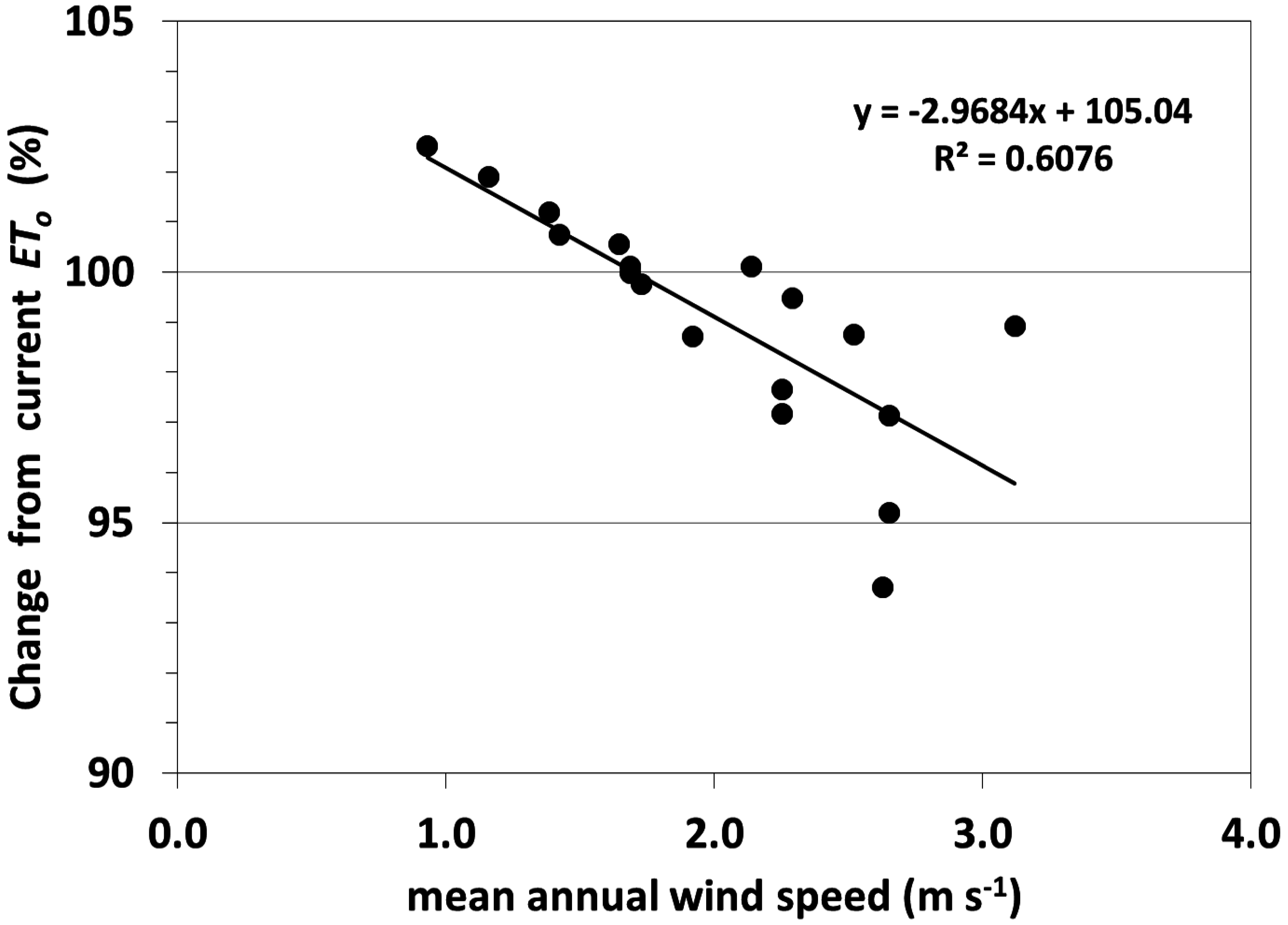
Using 18 California weather stations from a wide range of climates, daily data from 2003 were used to calculate how the annual ET_o might change with the aforementioned climate projections. The results (Figure 1) indicate that the climate change scenario would have little impact on annual ET_o. The annual ET_o increased slightly where there were mean wind speeds less than 1.7 m·s⁻¹, and it decreased for wind speeds greater than 1.7 m·s⁻¹. However, the absolute magnitude of variation from the current annual ET_o was small for all weather stations. Based on the regression lines in Figure 1, the 4 °C rise in T_d and the 17 s·m⁻¹ increase in r_c counteracted the impact of the 3 °C mean temperature increase.

6. Crop Coefficients

Allen et al. [7,8,11] reported a daily time step, standardized reference evapotranspiration equation for short canopies (Equation (7)). While the generated ET_o is actually for a virtual surface, i.e., having characteristics that determine the coefficients in Equation (4), the ET_o approximates the ET_c for a broad expanse of well-watered, cool-season grass. Allen et al. [7,8] also reported a daily time step equation for tall canopies (ET_r) that is expressed as

$$E{T}_r=\frac{0.408∆\left(R_n-G\right)+\frac{1600\gamma \left(e_s-e_a\right)u_2}{T+273}}{∆+\gamma \left(1+0.38u_2\right)} \left(\mathrm{mm}·{\mathrm{d}}^{-1}\right).$$

(9)

Note that Allen et al. [7] used r_c = 45 s·m⁻¹ and r_a = 118/u₂ to obtain the 0.38 = 45/118 in Equation (9). The canopy resistance for about 372 ppm CO₂ was derived using Equation (10) with r_s = 66.7 s·m⁻¹ and LAI = 2.96.

$$r_c=\frac{r_s}{0.5·LAI}=\frac{66.7 \mathrm{s}·{\mathrm{m}}^{-1} }{0.5\times 2.96}=45.1\approx 45 \mathrm{s}·{\mathrm{m}}^{-1}.$$

(10)

Assuming a 20% reduction in alfalfa stomatal conductance when changing from 372 to 550 ppm CO₂ [12], the stomatal conductance changes from 0.015 m·s⁻¹ to 0.012 m·s⁻¹, the stomatal resistance changes from 66.7 to 83.3 s·m⁻¹, and the canopy conductance at 550 ppm is estimated as

$$r_c=\frac{r_s}{0.5·LAI}=\frac{83.3 \mathrm{s}·{\mathrm{m}}^{-1} }{0.5\times 2.96}=56.3\approx 56 \mathrm{s}·{\mathrm{m}}^{-1} .$$

(11)

Strictly speaking, the ET_r equation estimates the ET_c for a virtual surface with characteristics represented by coefficients used in Equation (9), but the ET_r rates are approximately equal to the ET_c of a broad expanse of well-watered, 0.5-meter-tall alfalfa. Derivations and explanations of the ET_o and ET_r equations are addressed in [7,8]. To accurately estimate ET_o and ET_r, the input weather data for Equations (4)–(9) are collected over a broad expanse of well-watered grass. Derivation of the net radiation (R_n) and ground heat flux (G) in MJ·m⁻²·d⁻¹ are presented in [7]. The T (°C) is the mean air temperature measured at a height between 1.5 and 2.0 m, u₂ (m·s⁻¹) is the mean daily wind speed monitored at a 2 m height, the saturation vapor pressure (e_s) in kPa is calculated from T, and the actual vapor pressure (e_a) in kPa is measured at the same height as T. The slope of the saturation vapor pressure (∆) in kPa·°C⁻¹ and the psychrometric constant γ in kPa·°C⁻¹ are computed as described in [7].

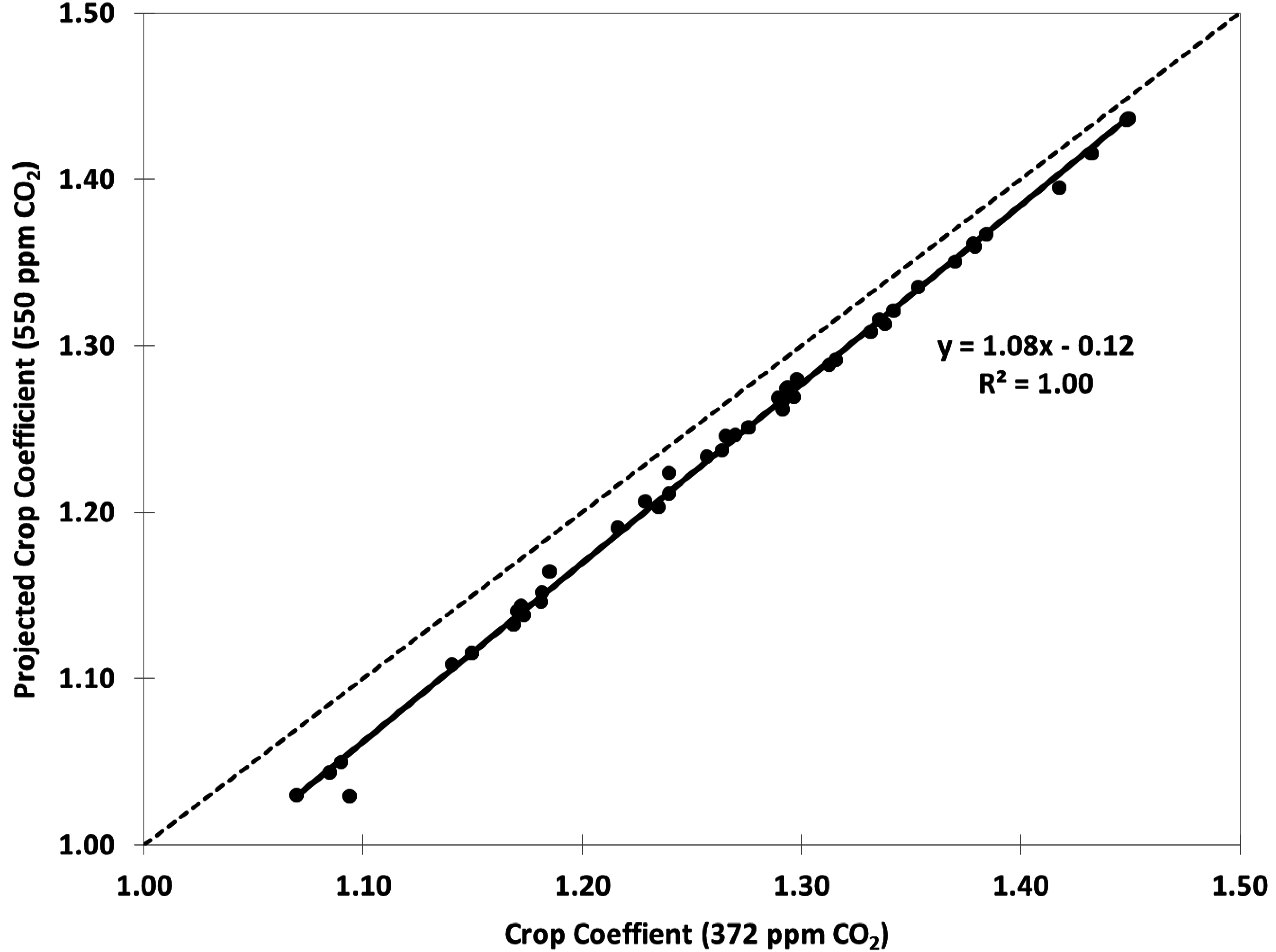
While little change in ET_o rates is expected due to global climate change, crop coefficient (K_c) values might be affected depending on how climate factors change in the future. To evaluate the effect of changing weather variables on K_c values, an analysis was done using data from 49 California Irrigation Management Information System (CIMIS) weather stations [16]. Equations (4) and (9) were used to compute ET_o and ET_r using canopy resistances corresponding to both 372 and 550 ppm CO₂. The stomatal conductances g_s = 0.010 m·s⁻¹ (grass) and g_s = 0.015 m·s⁻¹ (alfalfa) were reduced by 20% to 0.008 m·s⁻¹ (grass) and 0.012 m·s⁻¹ (alfalfa) at 550 ppm CO₂ based on [12]. The K_c for alfalfa was calculated for 372 ppm CO₂ for all 49 stations using the mean climate data from July 2003. For 550 ppm CO₂, the K_c for alfalfa was calculated using the mean climate data from July 2003, but with the monthly mean daily maximum, minimum, and dew point temperatures increased by 2 °C, 4 °C, and 4 °C, respectively. The wind speed and equations for aerodynamic resistance were not changed.

A plot of the 550 ppm versus 372 ppm K_c values (Figure 2) indicates that the crop coefficients are likely to decrease slightly for a wide range of climates. The biggest K_c decrease was about 0.03 when K_c ≈ 1.10, and the smallest decrease was about 0.01 for K_c ≈ 1.40. The differences were approximately 0.01 when K_c values were high. The response of K_c to the projected climate change is most likely related to the alfalfa canopy being more coupled with the environment than the grass canopy, which has a higher aerodynamic resistance. Plant canopies that are more coupled to the environment are more likely to exhibit a reduction in transpiration rate than a canopy that is more controlled by the aerodynamic resistance, e.g., grass. This analysis provides some evidence that coupling with the environment might lead to reductions in crop coefficients due to global climate change.

While changes in the CO₂ concentration can have an effect on the canopy resistance, this analysis showed that the same percentage decrease stomatal conductance can lead to a bigger reduction in transpiration if the aerodynamic resistance is lower and the canopy is more coupled with the environment. There is a lack of information on how crop coefficients of orchard and vine crops might respond to climate change, but the alfalfa example in this paper provides some insight. Since taller rougher canopies, e.g., orchards and vineyards, have considerably lower aerodynamic resistance than alfalfa, it is likely that the K_c values for orchard and vine crops might decrease even more.

For both C₄ and C₃ species, stomatal conductance is reduced by the increasing CO₂ concentration external to leaves [17]. However, small differences in C₄ and C₃ stomatal conductance responses to CO₂ concentration have been reported for grasses with the conductance differences decreasing at higher CO₂ concentrations [18]. On the other hand, grasses are more decoupled from the environment than taller, rougher plant canopies, so the K_c response of grass species due to a projected climate is likely to be smaller than the K_c response of taller rougher plant canopies with lower aerodynamic resistance.

7. Conclusions

In summary, the evidence for anthropogenic global climate change due to the excessive release of CO₂ into the atmosphere is strong. While there are many possible impacts of climate change on horticultural crops, the effect of changes on water use of horticultural crops is particularly important. The fact that global climate change is dependent only on global receipt and reflection of solar radiation and GHGs provides strong evidence that anthropogenic global climate change is real and concerning. The global change can impact many weather factors in addition to affecting physical and biological factors, and these weather factors can affect plant growth and agricultural production. The FACE studies showed that increasing atmospheric CO₂ will decrease stomatal conductance, and this will increase canopy resistance of C₃ species plants, which decreases plant transpiration. Additionally, climate change projections indicate that water vapor content of the air will increase as temperature rises, and increased atmospheric H₂O also decreases transpiration. Using the standardized reference evapotranspiration equation for short canopies to calculate ET_o, the impact of projected increases in atmospheric temperature and CO₂ and H₂O concentrations were evaluated, and a large effect on ET_o rates is unlikely. There was some evidence that ET_o would increase slightly at low wind speeds and it would decrease as wind speeds increased. The calculation of alfalfa K_c values at 372 and 550 ppm CO₂ with an increase of 2 °C, 4 °C, and 4 °C for maximum, minimum, and dew point temperatures in the higher CO₂ environment, showed that K_c values will probably slightly decrease. This decrease is likely due to the higher coupling of canopy to the environment for the alfalfa canopy. There is little information available about how K_c values might change for tree and vine crops, but trees and vines are even more coupled to the environment, so an even bigger decrease in K_c seems plausible for the taller rougher canopies. A similar K_c response to climate change is expected for both C₃ and C₄ plants. While the evapotranspiration responses to global change seem small, the projected changes in precipitation and water storage in snowpack are large and could have devastating impacts on horticulture in some regions.

References

- IPCC. Climate Change 2013. The Physical Science Basis Working Group I Contribution to the Fifth Assessment Report of the Intergovernmental Panel on Climate Change; Cambridge University Press: New York, NY, USA, 2014; pp. 1–1535. [Google Scholar]
- Dixon, G.R.; Collier, R.H.; Bhattacharya, I. An assessment of the effects of climate change on horticulture. In Horticulture: Plants for People and Places; Dixon, G.R., Aldous, D.E., Eds.; Springer: Dordrecht, The Netherlands, 2014; Volume 2, pp. 817–857. [Google Scholar]
- Glenn, D.M.; Kim, S.H.; Ramirez-Villegas, J.; Läderach, P. Response of Perennial Horticultural Crops to Climate Change. In Horticultural Reviews, 1st ed.; Janick, J., Ed.; John Wiley & Sons, Inc.: Hoboken, NJ, USA, 2013; Volume 41, pp. 47–129. [Google Scholar]
- Anderson, J.; Chung, F.; Anderson, M.; Brekke, L.; Easton, D.; Ejeta, M.; Peterson, R.; Snyder, R.L. Progress on incorporating climate change into management of California’s water resources. Clim. Chang. 2008, 87, S91–S108. [Google Scholar] [CrossRef]
- Arrhenius, S.A. On the Influence of Carbonic Acid in the Air Upon the Temperature of the Ground. Philos. Mag. J. Sci. 1896, 41, 237–276. [Google Scholar] [CrossRef]
- NOAA Layers of the Atmosphere. Available online: http://www.srh.noaa.gov/jetstream/atmos/layers.html (accessed on 18 November 2016).
- Allen, R.G.; Walter, I.A.; Elliott, R.L.; Howell, T.A.; Itenfisu, D.; Jensen, M.E.; Snyder, R.L. The ASCE Standardized Reference Evapotranspiration Equation; American Society of Civil Engineers: Reston, VA, USA, 2005; pp. 1–173. [Google Scholar]
- Allen, R.G.; Pruitt, W.O.; Wright, J.L.; Howell, T.A.; Ventura, F.; Snyder, R.L.; Itenfisu, D.; Steduto, P.; Berengena, J.; Baselga Yrisarry, J.; et al. A recommendation on standardized surface resistance for hourly calculation of reference ETo by the FAO56 Penman-Monteith method. Agric. Water Manag. 2006, 81, 1–22. [Google Scholar] [CrossRef]
- Monteith, J.L. Evaporation and Environment. Symp. Soc. Exp. Biol. 1965, 19, 205–234. [Google Scholar] [PubMed]
- Snyder, R.L.; Moratiel, R.; Zhenwei, S.; Swelam, A.; Jomaa, I.; Shapland, T. Evapotranspiration Response to Climate Change. Acta Hortic. 2011, 922, 91–98. [Google Scholar] [CrossRef]
- Allen, R.G.; Pereira, L.S.; Raes, D.; Smith, M. Crop Evapotranspiration: Guidelines for Computing Crop Water Requirements; Irrigation and Drainage Paper No. 56; FAO of United Nations: Rome, Italy, 1998; pp. 1–300. [Google Scholar]
- Long, S.P.; Ainsworth, E.A.; Rogers, A.; Ort, D.R. Rising atmospheric carbon dioxide: plants FACE the future. Ann. Rev. Plant Biol. 2004, 55, 591–628. [Google Scholar] [CrossRef] [PubMed]
- Cayan, D.; Luers, A.L.; Hanemann, M.; Franco, G. Scenarios of Climate Change in California: An Overview; CEC-500-2005-186-SF; California Energy Commission: Sacramento, CA, USA, 2006. [Google Scholar]
- Prentice, I.C.; Farquhar, G.D.; Fasham, M.J.R.; Goulden, M.L.; Heimann, M.; Jaramillo, V.J.; Kheshgi, H.S.; Le Quéré, C.; Scholes, R.J.; Wallace, D.W.R. The Carbon Cycle and Atmospheric Carbon Dioxide. In Climate Change 2001: The Scientific Basis. Contribution of Working Group I to the Third Assessment Report of the Intergovernmental Panel on Climate Change; Cambridge University: Cambridge, UK; New York, NY, USA, 2002; pp. 183–238. [Google Scholar]
- Roderick, M.L.; Farquhar, G.D. Changes in New Zealand Pan Evaporation since the 1970s. Int. J. Climatol. 2005, 25, 2031–2039. [Google Scholar] [CrossRef]
- Snyder, R.L.; Pruitt, W.O. Evapotranspiration Data Management in California; American Society of Civil Engineers: New York, NY, USA, 1992; pp. 128–133. [Google Scholar]
- Morison, J.I.L.; Gifford, R.M. Plant growth and water use with limited water supply in high CO2 concentrations. I. Leaf area, water use and transpiration. Aust. J. Plant Physiol. 1984, 11, 361–374. [Google Scholar]
- Hager, H.A.; Ryan, G.D.; Kovacs, H.M.; Newman, J.A. Effects of elevated CO2 on photosynthetic traits of native and invasive C3 and C4 grasses. BMC Ecol. 2016, 16, 28. [Google Scholar] [CrossRef] [PubMed]
Figure 1.
A plot of the change from current annual ETo (mm·y−1) assuming Tx increases by 2 °C, Tn increases by 4 °C, Td increases by 4 °C, and rc increases from 70 to 87 s·m−1 versus the mean annual wind speed. Figure 1 is from Snyder et al. [10].
Figure 2.
A plot of Kc values for alfalfa calculated from July 2003 mean daily weather data from 49 CIMIS weather stations in California for a climate with 550 ppm versus 372 ppm CO2. For the projected 550 ppm CO2 climate, the original daily maximum temperature data were increased by 2 °C, and the minimum and dew point temperatures were increased by 4 °C relative to July 2003 data. The wind speed and solar radiation were not changed from the original data. The alfalfa ETc was computed using the ETr equation (Equation (9)), and ETo was computed using Equation (4).
© 2017 by the author. Licensee MDPI, Basel, Switzerland. This article is an open access article distributed under the terms and conditions of the Creative Commons Attribution (CC BY) license (http://creativecommons.org/licenses/by/4.0/).
Share and Cite
MDPI and ACS Style
Snyder, R.L. Climate Change Impacts on Water Use in Horticulture. Horticulturae 2017, 3, 27. https://doi.org/10.3390/horticulturae3020027
AMA Style
Snyder RL. Climate Change Impacts on Water Use in Horticulture. Horticulturae. 2017; 3(2):27. https://doi.org/10.3390/horticulturae3020027
Chicago/Turabian StyleSnyder, Richard L. 2017. "Climate Change Impacts on Water Use in Horticulture" Horticulturae 3, no. 2: 27. https://doi.org/10.3390/horticulturae3020027
Note that from the first issue of 2016, this journal uses article numbers instead of page numbers. See further details here.