Performance Analysis of Machine-Learning Approaches for Modeling the Charging/Discharging Profiles of Stationary Battery Systems with Non-Uniform Cell Aging

Abstract

The number of Stationary Battery Systems (SBS) connected to various power distribution networks across the world has increased drastically. The increase in the integration of renewable energy sources is one of the major contributors to the increase in the number of SBS. SBS are also used in other applications such as peak load management, load-shifting, voltage regulation and power quality improvement. Accurately modeling the charging/discharging characteristics of such SBS at various instances (charging/discharging profile) is vital for many applications. Capacity loss due to the aging of the batteries is an important factor to be considered for estimating the charging/discharging profile of SBS more accurately. Empirical modeling is a common approach used in the literature for estimating capacity loss, which is further used for estimating the charging/discharging profiles of SBS. However, in the case of SBS used for renewable integration and other grid related applications, machine-learning (ML) based models provide extreme flexibility and require minimal resources for implementation. The models can even leverage existing smart meter data to estimate the charging/discharging profile of SBS. In this paper, an analysis on the performance of different ML approaches that can be applied for lithium iron phosphate battery systems and vanadium redox flow battery systems used as SBS is presented for the scenarios where the aging of individual cells is non-uniform.

1. Introduction

Leon Walker’s research in the field of Stationary Battery Systems (SBS) has shown that, in comparison with the batteries used for consumer and automotive applications, the market share of SBS is significantly lower [1]. However, there is a steady increase in the total installed capacity of SBS, which in 2023 is expected to reach a market value of approximately USD 13 billion [2]. Primarily, SBS can be categorized into three major areas: renewable energy, auxiliary services for the grid and uninterrupted power supplies. In recent times, the prolific growth of SBS capacity installed in distribution networks is largely attributed to the policies for climate change in various countries across the world, and Singapore is one such country. Because of several initiatives taken to counterbalance rapid climate change, there is a significant increase in integration of different intermittent renewable energy sources like solar photo-voltaics (PVs). Singapore, for instance, is one of the cities where solar PV integration into the distribution network has seen a prolific growth in recent years [3,4]. Also, there have been tenders released by the Singaporean government in favor of increasing the installation of solar PVs to public sector buildings and various Housing Development Board blocks across the city in 2016, and by 2020 the government aims to obtain a solar PV capacity of 350 MWp [3].

Large-scale integration of such intermittent renewable energy sources would have negative impacts on the distribution network’s stability and reliability [5,6,7,8,9,10]. Thus, for such cases, SBS can be used as a buffer which will considerably reduce power output variability along with improving stability and reliability [11,12,13]. In addition, SBS can also provide other benefits for utilities, including peak load management, load-shifting applications (peak shaving and valley filling), voltage regulation and power quality improvement [14]. The Energy Market Authority of Singapore and Singapore Power jointly launched the “Energy Storage Programme” [15] to evaluate utility-scale energy storage systems (ESS) for such applications. Furthermore, there is also a significant contribution from other type of distributed storage in electrical appliances that use solar energy, like refrigerators, air conditioners, and lighting fixtures. Introduction of distributed storage systems like Tesla’s Powerwall and use of the second life of automotive batteries [16] for reducing energy costs will contribute considerably to an increase in the installed capacity of SBS. Generally, the operation of the SBS is done consecutively as a source and load while functions such as load shifting are being executed. Hence, there are variations on the charging/discharging profile of storage devices that are completed under different parameters like initial state of charge (SOC), final desired SOC, storage device type and charging/discharging cycles (corresponds to capacity loss). Accurately determining the charging/discharging profiles of such storage devices connected to a distribution network will enable various energy management applications such as maximum demand prediction, load scheduling and demand response management.

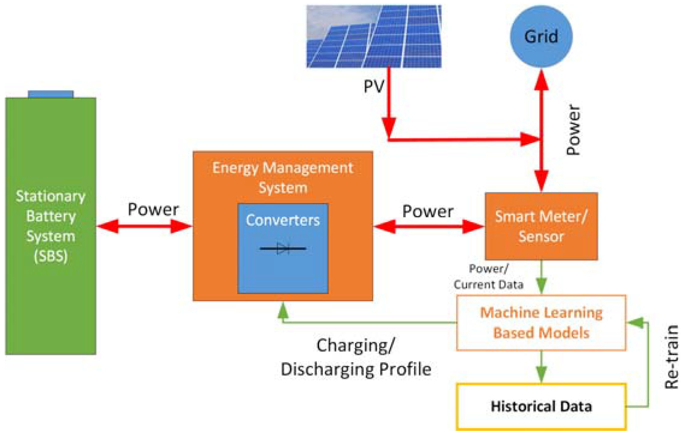
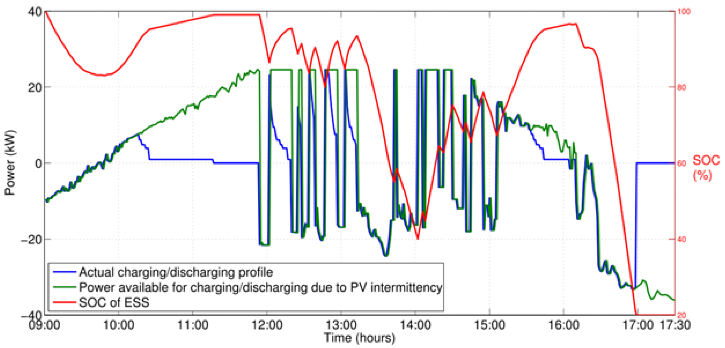
Need for Predicting the Charging/DischargingPprofile

Consider an SBS with 24 kWh battery energy capacity and 48 kW power capacity for a typical roof top PV of 70 kWpeak (size of the SBS is not considered in this scope). The difference between charging/discharging power available due to the intermittency of solar PV and the actual charging/discharging profile of the SBS due to the limitations imposed by constant current (CC) and constant voltage (CV) regions are shown in Figure 1. It is evident from Figure 1 that it is crucial to determine the charging/discharging profiles accurately. The calculations for PV power are shown in Appendix A, and it is assumed that the PV power should be maintained at the average power generated over the day.

2. Literature Review

The charging of SBS is a non-linear process and changes regularly due to the change in chemical composition of the device [17,18]. Capacity loss due to the aging process is an important factor that affects the charging profiles of any SBS [17,18]. There are numerous aging models available in the literature, and the authors have studied the impact of various parameters such as charge/discharge rate, depth of discharge, temperature and calendar aging [19]. The authors of [17,18] and [20,21,22] have studied the aging process of lithium ion and vanadium flow batteries using empirical and physical models. The aging model proposed in [18] for a lithium iron phosphate (LFP) battery was based on accelerated aging, and it is used as a reference model in this paper. The aging model proposed in [23] for a vanadium redox flow battery (VRB) was based on fixed aging and is used as reference model in this paper. The models can be utilized for determining the capacity fade and could be combined with the charging power/current model proposed in [24] to determine the theoretical charging power/current of the whole charging process of any SBS. However, the constants derived based on the accelerated ageing process depend on various operating parameters such as temperature, usage pattern, location of the device, etc., so the parameters would vary among the cells in the same battery pack. SBS deployed in smart grids have the inherent advantage that power/current consumption data is continuously monitored, and in such cases machine-learning (ML) based modeling could be used to determine the charging/discharging profiles of SBS [24,25] (a black box approach). However, it is to be noted that generally an SBS is built connecting large number of individual cells in a series/parallel combination and the aging process of such cells is usually non-uniform [26]. Hence, any black box modeling approach should be capable of capturing the changes in such abnormalities due to non-uniform aging process. Though, ML approaches are used for modeling battery cells [27,28,29], an evaluation of the performance for identifying non-uniform aging of cells at the pack level has not been carried out.

In this paper, ML models based on Artificial Neural Networks (ANN) and Ensemble Learning methods are used to determine the charging/discharging profiles of SBS in which the aging of individual cells are non-uniform. Performance evaluations are carried out for the cases where the aging of individual cells are not uniform. It is to be noted that the contribution of the paper pertains to the approaches used for determining the charging/discharging profile or load demand of SBS and the analysis of the performance rather than the ML models. Leveraging the existing data is an important aspect that would add value to the smart grid infrastructure. To summarize the contributions of this paper, we study the application and comparison of different types of ML models that can be used for SBS and analyze the performance of the models under scenarios where the aging of individual cell is non-uniform. The architecture of the proposed system is presented in Figure 2 for a typical PV application.

3. Models for Simulating Charging/Discharging Profiles

3.1. Lithium Iron Phosphate Batteries

The capacity fade model for LFP batteries proposed in [18] and charging power model proposed in [24] are given below in Equations (1)–(4),

$$C_{fade,k}=0.021\times e^{(-0.01943\times {\varphi }_k\times A{h}_{av})}\times C{d}^{0.7162}\times N{c}^{0.5}$$

(1)

where $C_{fade,k}$ represents the capacity fade (%) of kth cell, $A{h}_{av}$ represents the average Ah/SOC of the SBS during the current cycle, $Cd$ is the cycle depth or depth of discharge of the current cycle, ${\varphi }_k$ is constant which can used to realize non-uniform capacity fade among different cells and $Nc$ is the number of cycles. The charging current in the CC mode is given by

$$I_n=\frac{I_{cc}}{\eta }-(0.05\times \frac{I_{cc}}{\eta })+(W\times 0.01)$$

(2)

where $I_n$ is the current supplied at any instant (negative value is used for discharging), $I_{cc}$ is the current required in CC mode, $W$ is a pseudo-random integer variable uniformly distributed over an interval [0, 1], η is the converter efficiency (considered as 0.95) and $n$ is any instant in the charging process. $W$ is used as a parameter with which the variability introduced by the power electronic converters employed for charging/discharging the SBS can be realized. The charging current in CV mode is given by

$$I_n=I_{n-1}-I_{slope}$$

(3)

where $I_{slope}$ is the slope of current decrement which can be calculated using time required for CV mode. The increment in Ah is calculated using the equation below,

$$A{h}_{new}=A{h}_{old}+[\frac{I_n}{I_{1C}}\times 100]$$

(4)

where $A{h}_{new}$ is the increase in Ah or energy stored, $A{h}_{old}$ is the before supplying $I_n$, $I_{1C}$ is the current requirement for charging the battery at the rate of 1C It is to be noted that all the currents mentioned are on the AC side.

The impact of having different values for $\varphi$ with a 60 Ah LFP cell is shown in Figure 3; the cycle depth $Cd$ is considered constant at 80%. It can be observed that when the value of $\varphi$ is changed from 0.25 to 2.5 the number of cycles changes from 71 to 3648. Hence, the value of $\varphi$ can be used to simulate non-uniform aging of cells. The specifications of the LFP cell used are given

Table 1. Specifications of the 60 Ah LFP cell.

Model-SP-LFP60AHA(A)
Nominal Capacity	60 Ah, 192 Wh
Nominal Voltage	3.2 V
Standard Current	0.3 C, 18 A
Max CC	3 C, 180 A
Self-Discharge	≤3%

.

A SBS consisting of 125 SP-LFP60AHA(A) cells is considered for the evaluation. Non-uniform aging is assigned for the cells; for example in scale 1, the 63rd cell is assumed to have minimum aging with ${\varphi }_k$ = 2.25 and the 1st cell and 125th cell have maximum aging with ${\varphi }_k$ = 2.15. Similarly, the values of ${\varphi }_k$ are varied between 1.0 and 2.25 and the value of ${\varphi }_k$ for different cells under both the scales are shown in Figure 4. Scale 1 represents a lower non-uniformity among the cells whereas scale 2 represents a higher non-uniformity.

The charging profiles of the SBS (LFP) are shown for the 50th, 550th, 1050th and 1550th cycles in Figure 5. A constant current charging/discharging (1C) is assumed for the simulation. The charging process is stopped once any one of the cell reaches its 100% Ah capacity and the discharging process is stopped once any one of the cell reaches 20% Ah capacity. It is to be noted that the capacity fade due to the cyclic effect is considered in each cycle and the cells are updated correspondingly. The effect of having non-uniform aging among cells can be seen in Figure 5. It can be observed that there is a significant reduction in the time required for completing the CV region with an increase in the number of cycles. This is because, with an increase in number of cycles, the capacity of the SBS decreases, as does the energy required in the CV region. However, the converters are designed to charge the SBS with the value of current irrespective of its age. Thus, higher current supplied from the converter and lower energy requirements result in a reduction of the time required for completing the CV region.

3.2. Vanadium Redox Flow Batteries (VRB)

The capacity fade model for VRB proposed in [23] is used in this paper as the reference model; it is given in Equation (5).

$$C_{fade,k}=0.021\times C{d}^{0.7162}\times {\varphi }_k$$

(5)

where $C_{fade,k}$ represents the capacity fade (%) of kth cell. $Cd$ is the cycle or depth of discharge of the current cycle depth, ${\varphi }_k$ is constant which can used to realize non-uniform capacity fade among different cells. The charging current equation is same as Equation (2). As the CV region is usually not required for VRB, $I_{cc}$ is used for the whole charging period as well as the discharging period. The value of ${\varphi }_k$ is varied between 1 and 1.67, similar to the case of LFP and is shown in Figure 6.

The charging profiles of the SBS (VRB) are shown for the 1000th, 2500th, 4000th and 5500th cycles in Figure 7. A constant current charging/discharging (1C) is assumed for the simulation. The charging process is stopped once any of the cells reaches its 100% Ah capacity, and the discharging process is stopped once any of the cells reaches 20% Ah capacity. It is to be noted that the capacity fade due to the cyclic effect is considered in each cycle and the cells are updated correspondingly. The effect of having non-uniform aging among cells can be visualized from Figure 7. Since VRB can be charged with constant current until 100%, the phenomenon described in LFP (reduction in time required for CV region) is not observed in the case of VRB.

4. Machine-Learning (ML) Approaches

ML approaches for modeling charging/discharging profiles are attractive because the default capabilities required for implementing ML algorithms are usually a part of the energy management systems (EMS). The capabilities required for implementing ML models are smart meter/sensor data, high volume of data storage, and powerful data analytic tools. ML approaches are flexible, requires minimal resources, adaptive to any of the changes in the system. Modeling can be carried out based on the extent of data available and is relatively less complex. Various ML tasks such as pattern recognition, clustering and classification are suitable for modeling the charging/discharging profiles of SBS.

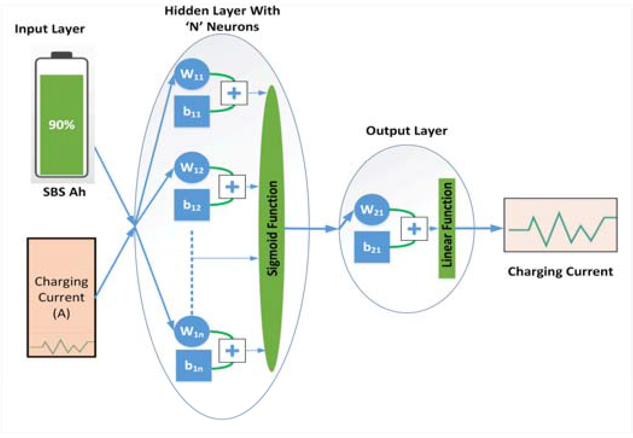
4.1. Model Based on an Artificial Neural Network with Feed-Forward Network and Back-Propagation as Training Algorithm

An ANN-based fitting model consisting of one input layer, a hidden layer and an output layer (feed-forward network) can be used for modeling the charging/discharging behavior of an SBS. The feed-forward network is designed with a sigmoid activation function for hidden neurons and linear activation function for output neurons. This is a standard network, which has the capability to fit multi-dimensional mapping problems arbitrarily well. However, consistency of the data and the sufficiency of neurons in hidden layer play a critical role. In this paper, the network is trained using the Bayesian regularization algorithm. This algorithm typically takes more time (~20 s in this case), but can result in good generalization for difficult, small or noisy data sets. Training stops based on adaptive weight minimization (regularization). The number of hidden neurons is considered as 10. The structure of the network used is shown in Figure 8.

The equations governing the model are given by

$$H_f=f\left({\displaystyle \sum _{i=1}^n(W_{1,i}\times Ah)+b_{1,i}}\right)$$

(6)

$$O_f=f\left({\displaystyle \sum _{i=1}^n(W_{2,i}\times H_f)+b_{2,1}}\right)$$

(7)

$H_f$ is the output of hidden layer where $W_{1,i}$ is the weight of i^th hidden neuron and $b_{1,i}$ is its corresponding bias. $O_f$ is the output of output layer (predicted current) where $W_{2,i}$ is the weight and $b_{2,i}$ is its corresponding bias. The inputs required are obtained from previous charging profiles.

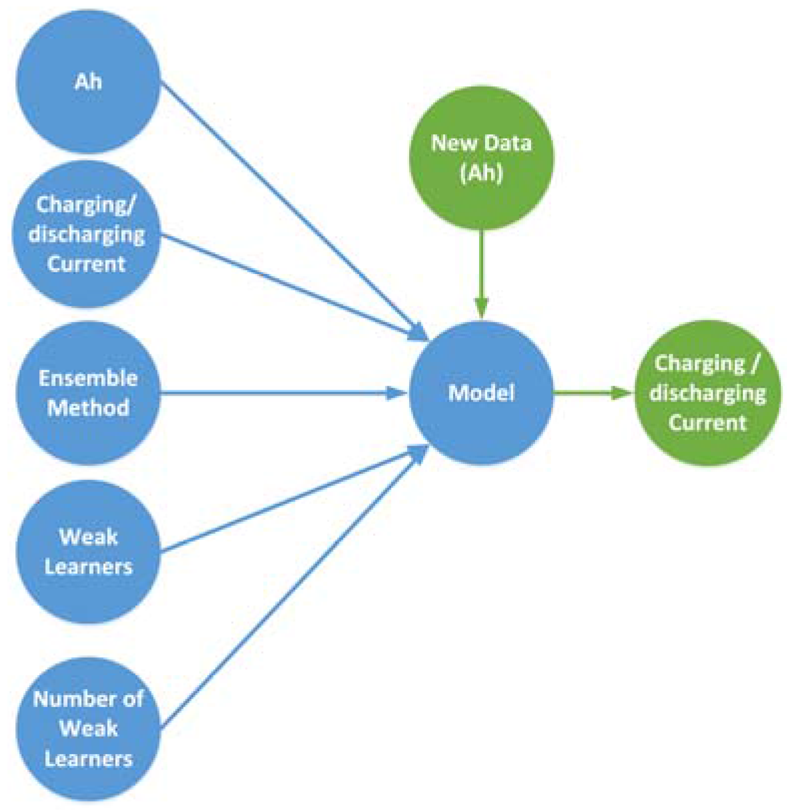
4.2. Model Based on Ensemble Learning (Least Square Boosting)

Ensemble learning is a type of machine learning process in which multiple learning algorithms are used to obtain a better prediction superior to the results obtained by using of any of the individual constituent learning algorithms alone. In the boosting method, the ensemble is built incrementally; emphasis is given to instances where training using previous models resulted in a mis-classification. Boosting yields better accuracy compared to bagging in some cases, although it is likely to over-fit the training data. The least square boost is used for the proposed application. In this method, the difference between the output obtained and the aggregated prediction of all learners in the previous steps is fitted with the new learner. “Tree” type learners are used and the number of weak learners is considered to be 100. The structure used is shown in Figure 9. The equations governing the model are given by

$$F_{(m+1)}(x)=F_m(x)+h(x)$$

(8)

$$h(x)=y-F_m(x)$$

(9)

$F_{(m+1)}(x)$ is the model/predictor at the current iteration, $F_m(x)$ is the model/predictor at the previous stage ($x$ is the Ah and $F_{(m+1)}(x)$ is the predicted charging current). It can be observed from the above equations that the accuracy of the model is improved at each iteration by fitting the residual from the previous iteration. The inputs required are obtained from previous charging profiles.

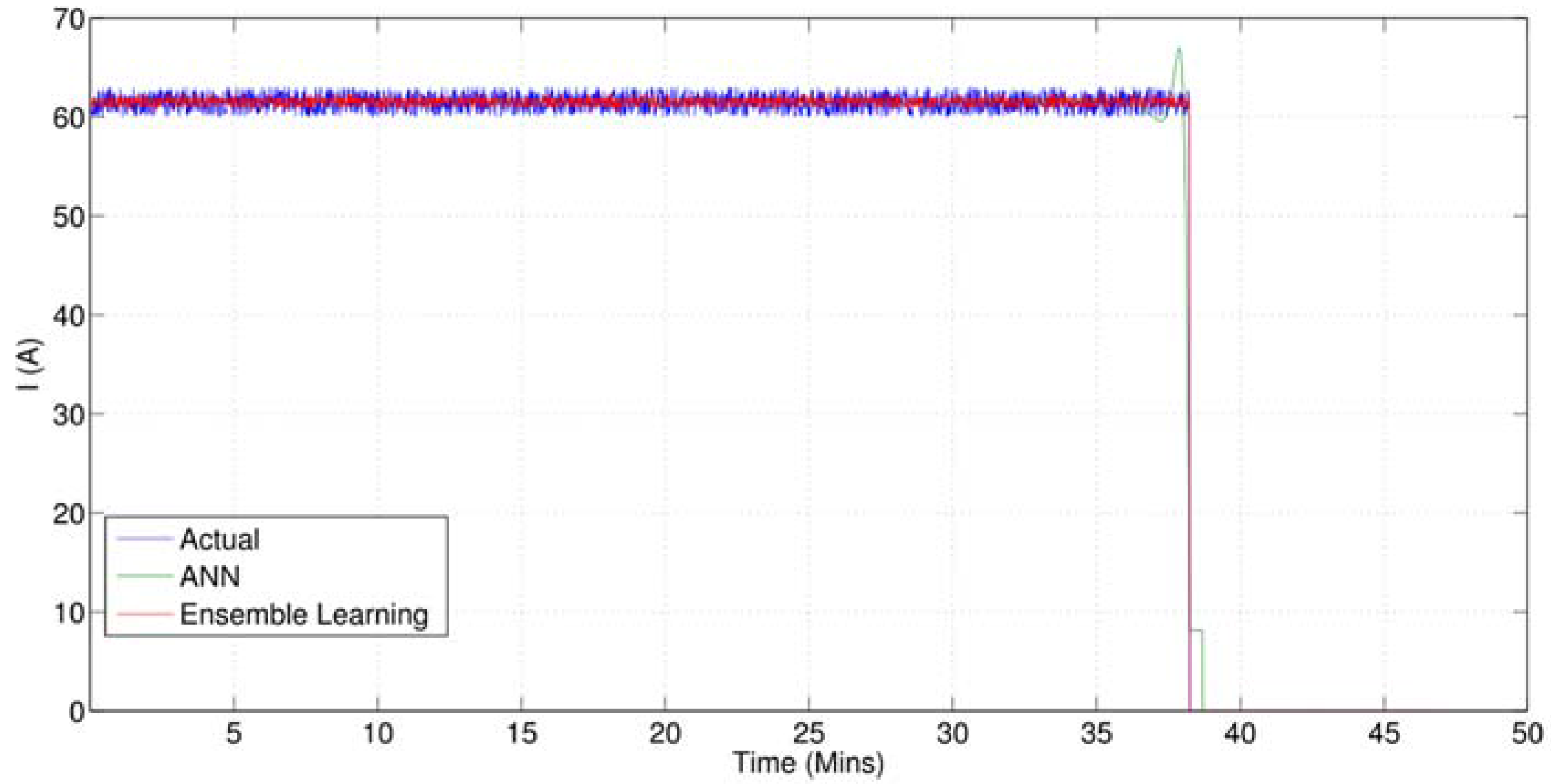
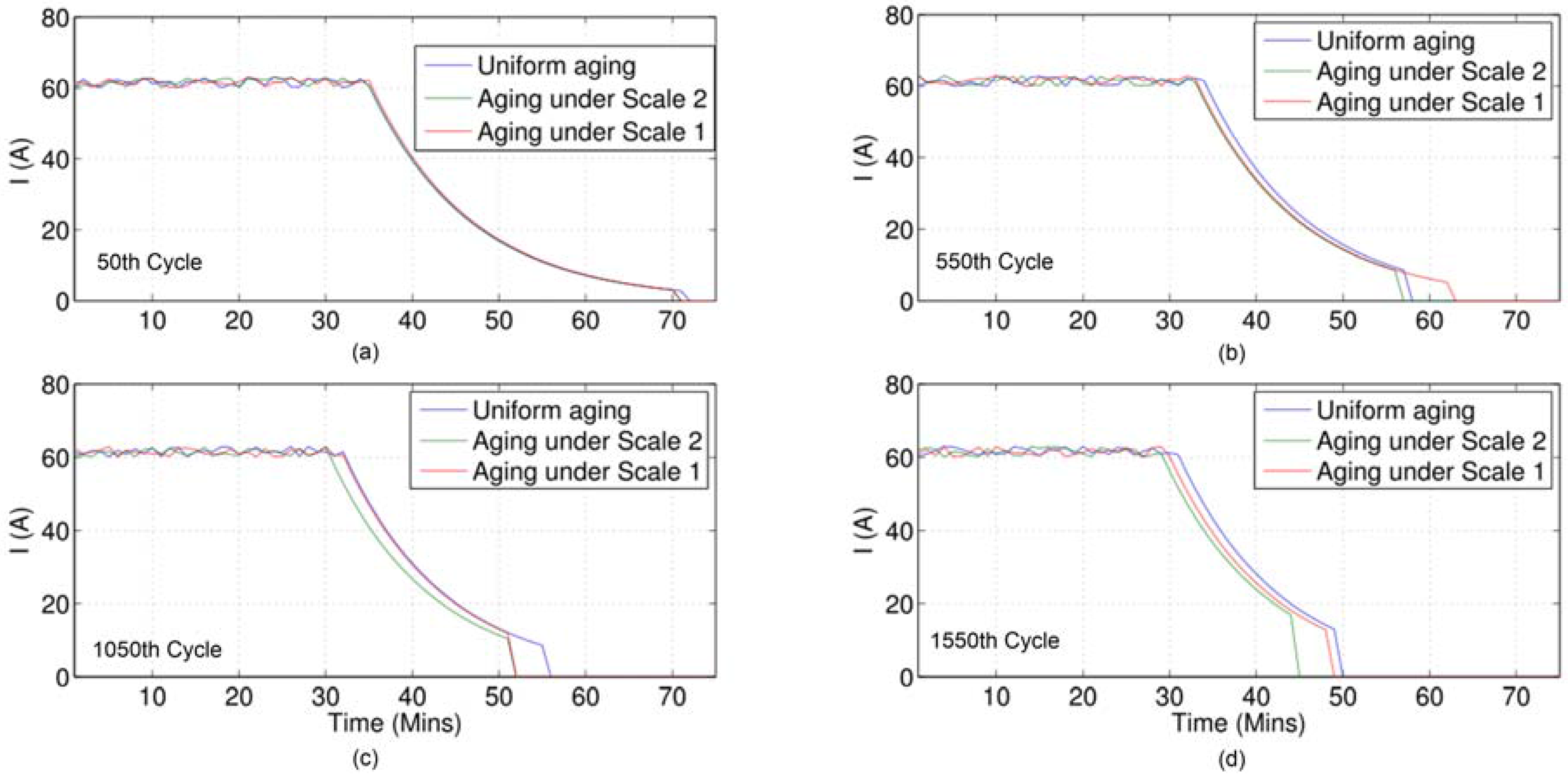
5. Simulation Results and Discussion

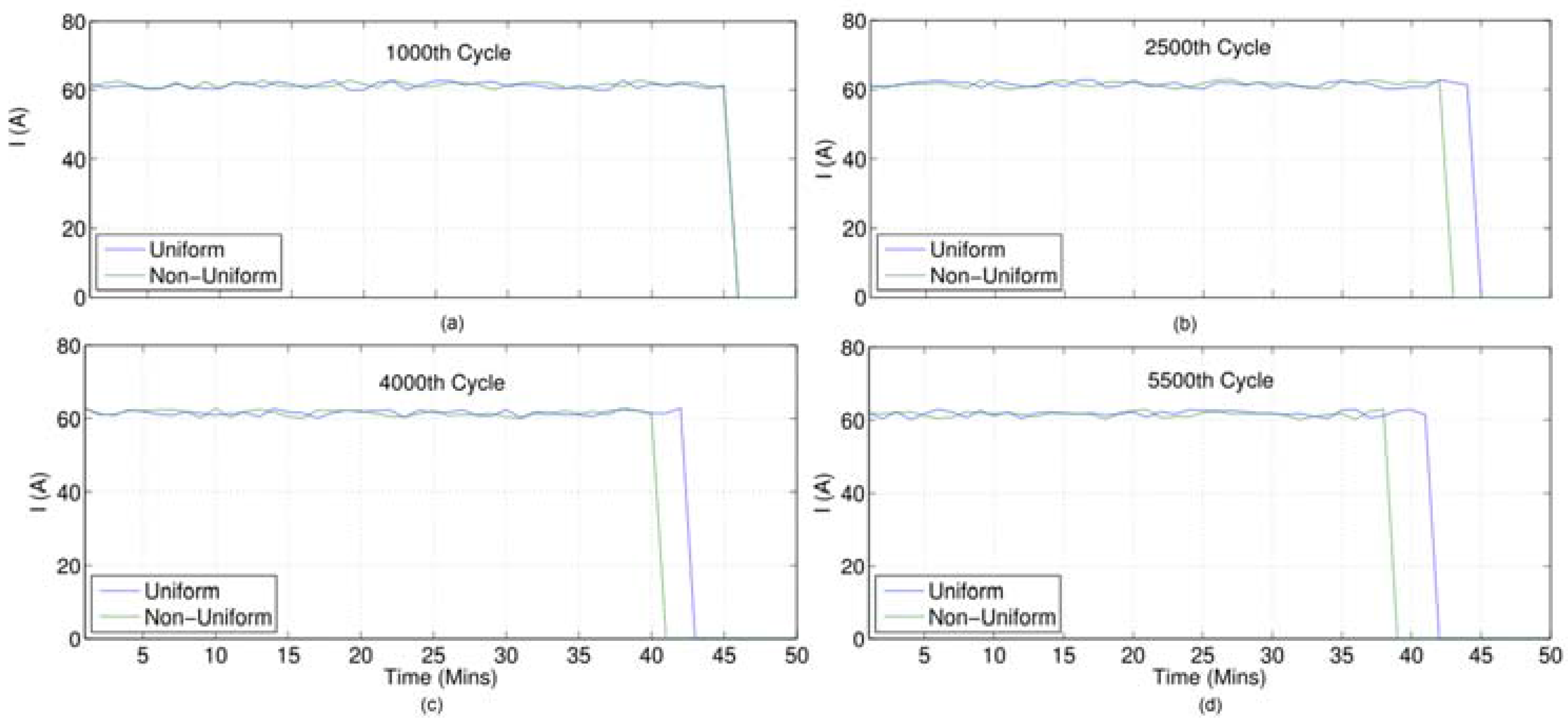
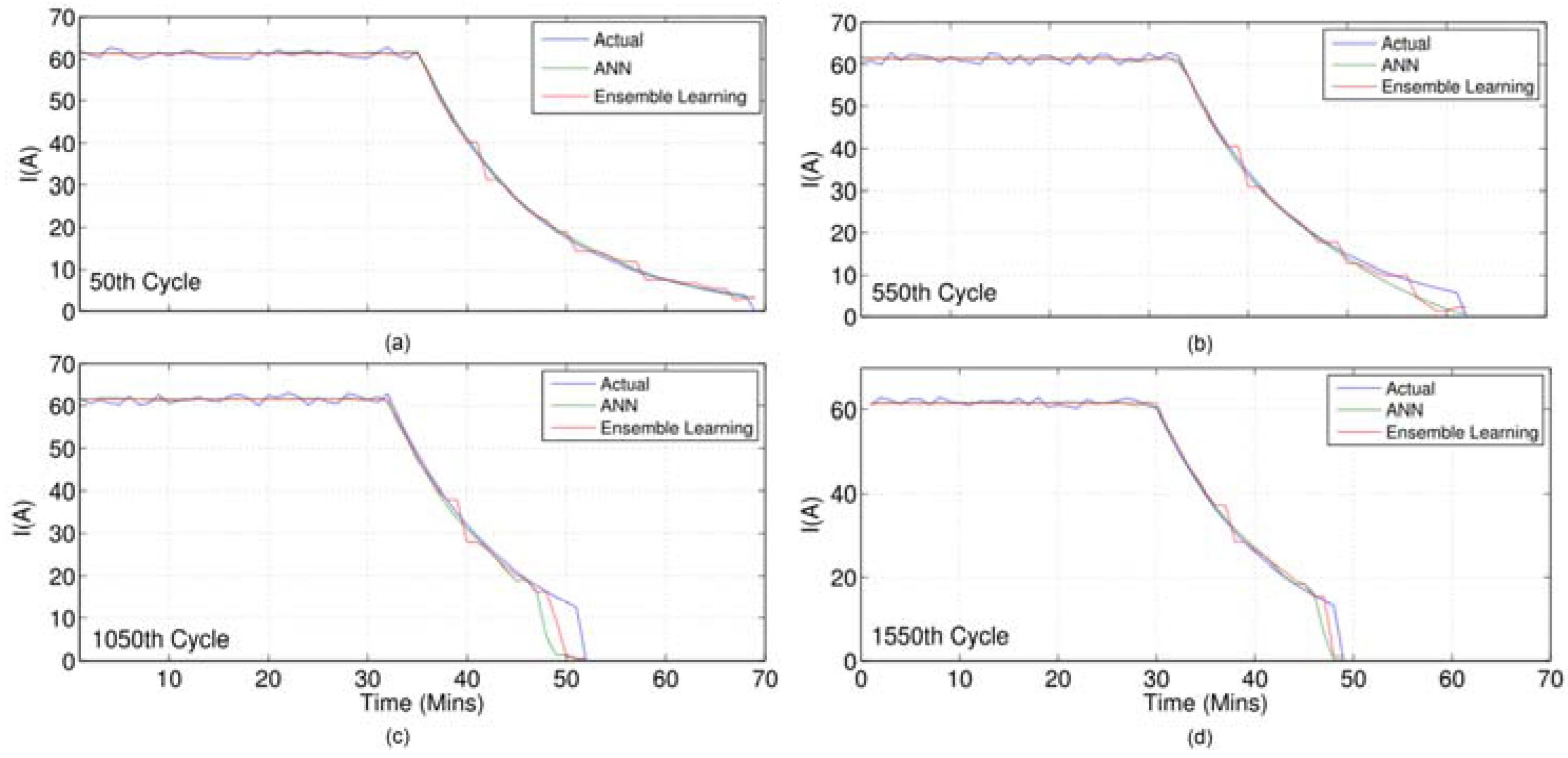
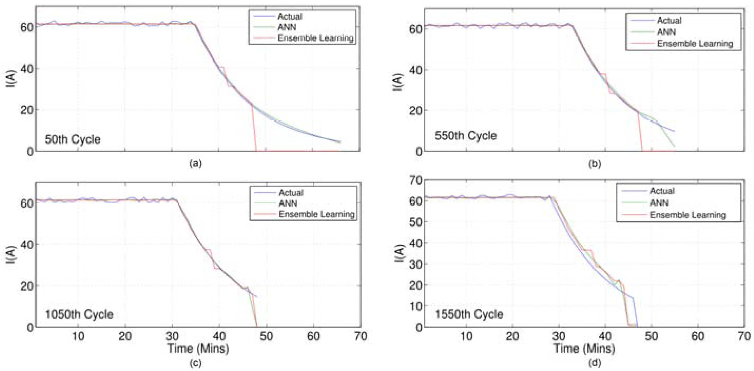
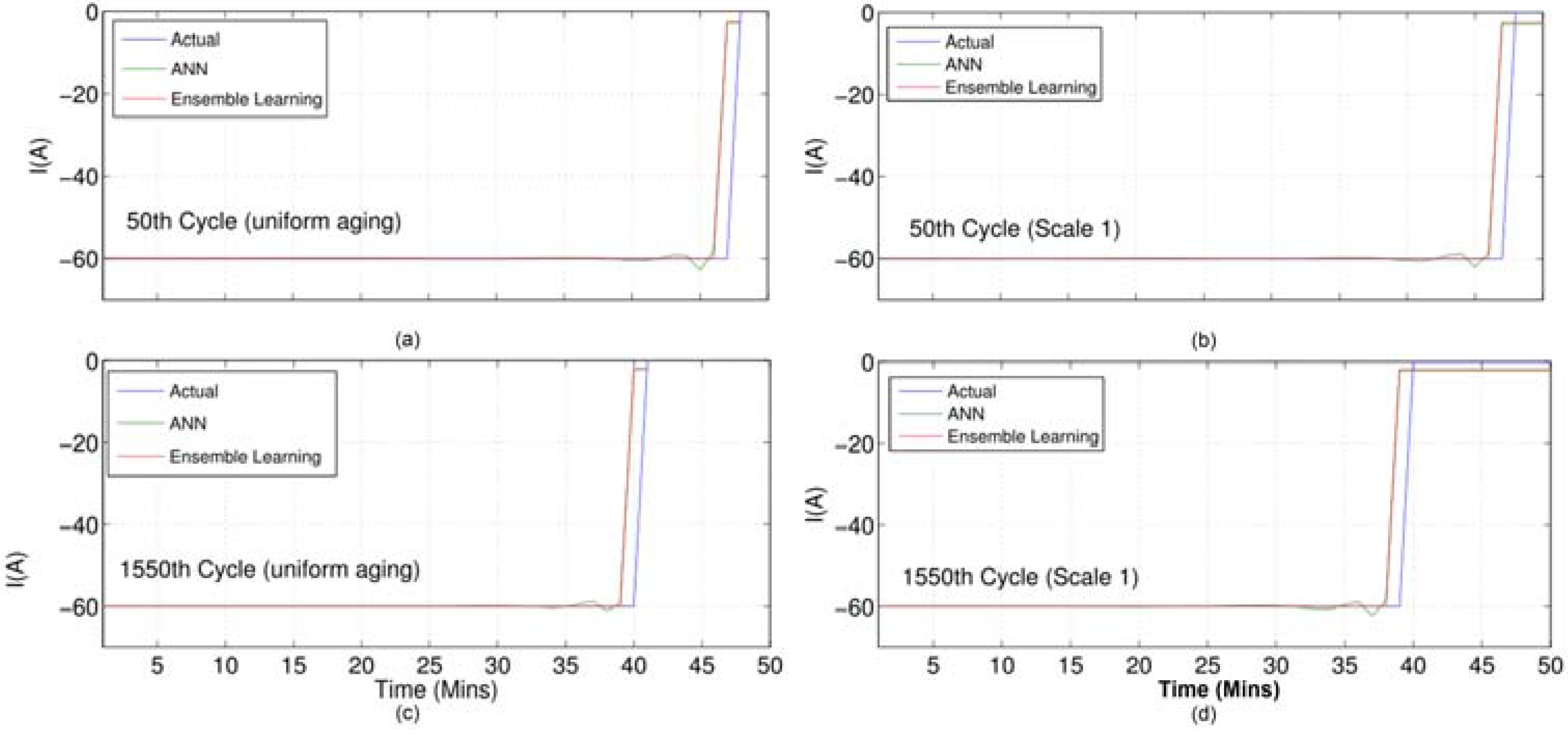
5.1. Lithium Iron Phosphate Batteries

The charging and discharging of the battery pack with ‘125’ SP-LFP60AHA(A) cells is simulated for uniform aging, non-uniform aging under scale 1 and scale 2 of Figure 4 until the capacity of any one cell reaches 80% of its original value. The prediction of charging is carried out for 50th, 550th, 1050th and 1550th cycle using both the ML models for all three cases. The results for charging profiles predictions are presented in Figure 10, Figure 11 and Figure 12. In the Figure 10, Figure 11 and Figure 12, the actual curve represents the simulated profile (indicated in blue) and the other two curves represent the predicted charging profile. The prediction is carried out for the whole charging period for all the cycles presented in the paper. The prediction of discharging is carried out for 50th and 1550th cycle (uniform aging and Scale 1), and the results are presented in Figure 13. The negative sign for current indicates discharging. From Figure 10, Figure 11 and Figure 12, it is evident that ANN generates a better prediction for the complete charging period. The performance of ensemble learning model is similar to ANN in the CC region, however, the error increases in the CV region. ANN provides a better performance in the CV region. It is also to be noted that the error of both the models not only increases with aging/number of cycles but also with the increase in non-uniformity in the aging of the cells. Furthermore, the ensemble learning model suffers from over fitting in few cases and cab be clearly observed in 50th cycle of Figure 12.

It is to be noted that since CC discharging is used and since there is no CV region while discharging, a superior performance is observed for the case of discharging profile prediction as observed from Figure 13. Higher accuracy in the prediction of discharging profiles can be attributed to the absence of non-linearity, as in the case of charging profiles. Furthermore, the performance of the ensemble learning model is better than ANN in predicting the discharging current, as ANN usually has a small error at the end of the discharging profile. An important observation is that with both the methods there is a fixed error at the extreme end of the Ah, i.e., 100% Ah (while charging) and 20% Ah (while discharging).

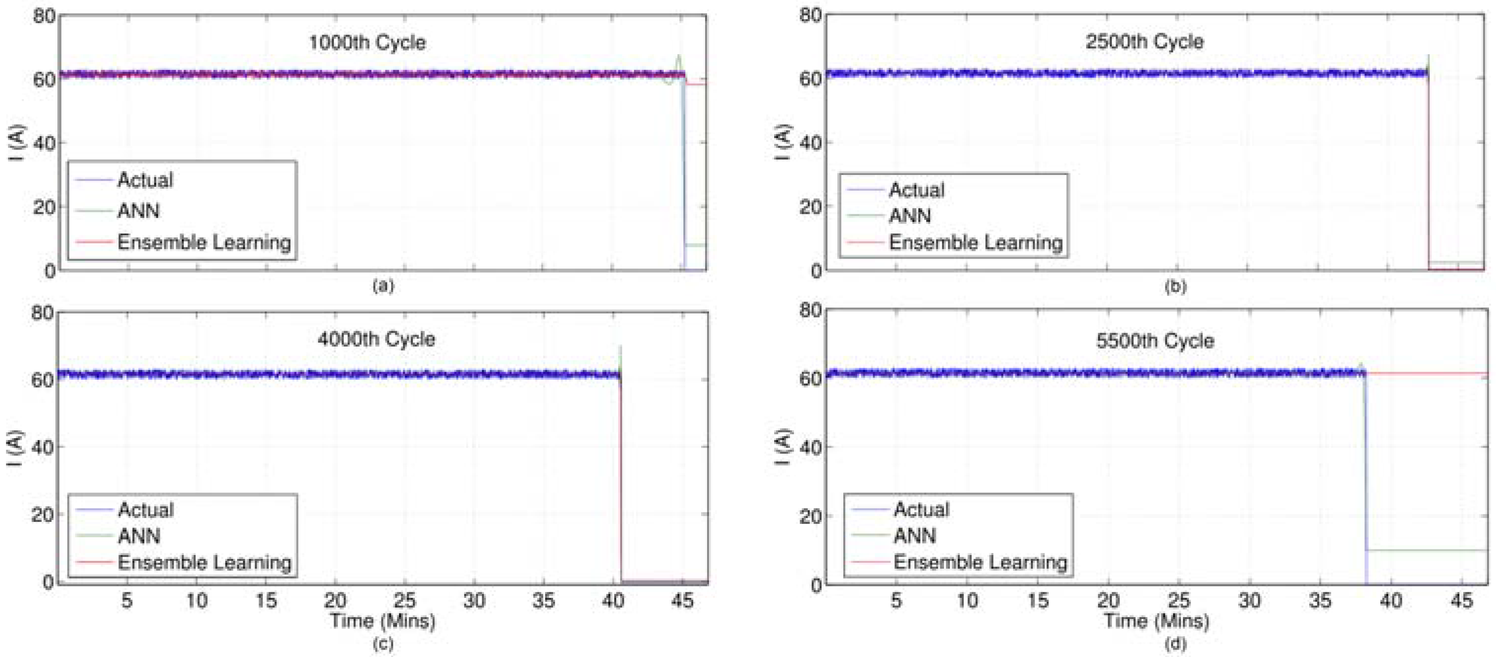
5.2. Vanadium Redox Flow Batteries

The charging and discharging of a battery pack with 125 cells is simulated for uniform aging and non-uniform aging as shown in Figure 6 until the capacity of any one cell reaches 80% of its original value. The prediction of charging profile is carried out for the 1000th and 6000th cycles using both the ML models for uniform and non-uniform aging. The prediction results are presented for charging in Figure 14; however, owing to symmetry for the results, discharging is not presented. The performance of the ML algorithms both in predicting charging and in discharging profiles is similar to that of discharging cases in LFP. This is due to the fact that no non-linear charging/discharging is considered (or practiced) for VRB.

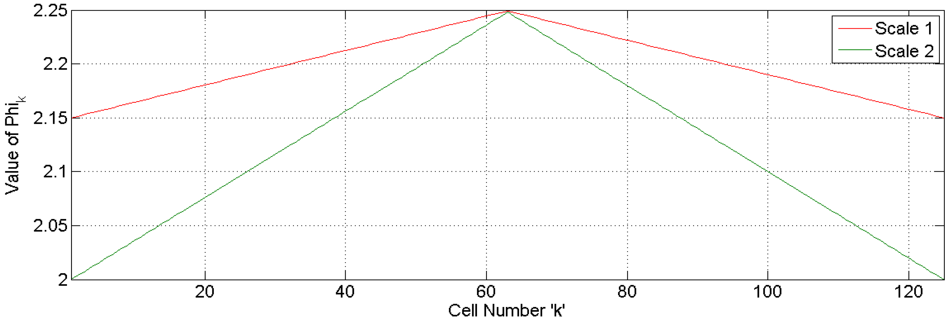
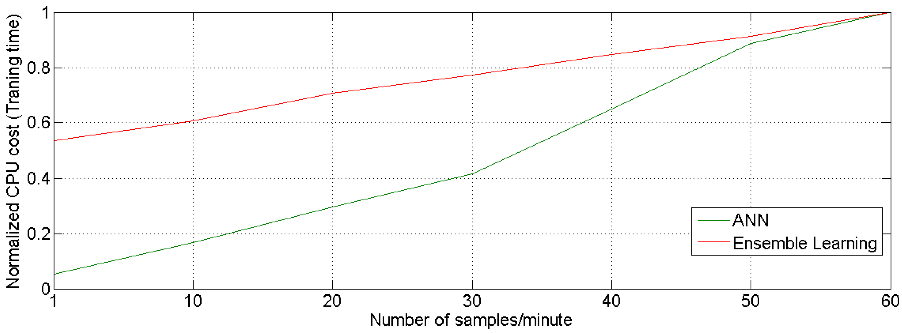
5.3. Impact of Sample Size and Other Model Parameters

In all the above simulations, a sample size of one sample/minute is used, and with the increase in sample size the accuracy also increases. The prediction results with increased sample size i.e., one sample/second is shown in Figure 15 for the 1000th, 2500th, 4000th and 5500th cycles under non-uniform aging. It can be observed that the accuracy is significantly improved as compared to sample size of one sample/minute. For ANN training, since more data is available, Levenberg-Marquardt back propagation is used as the training algorithm in place of Bayesian Regularization algorithm. The number of hidden neurons is increased to 20. In the case of ensemble learning, bagging is used instead of least square boosting. “Tree” type learners are used and the number of weak learners is maintained at 100. It can be inferred from Figure 15 that ANN generates more reliable predictions in all the cases, whereas boosting or bagging results in over fitting on some cases (similar to the case of Figure 12). However, it should be noted that the training time/prediction time depends on the sample size, algorithm and the parameters chosen for the algorithm. For example, Figure 16 shows the normalized CPU cost (training time) as a function of sample size in a typical case; for both ANN and Ensemble learning methods. A linear increase in the CPU cost can be observed for both the methods, however, the rate of change is different. Optimal sample size should be selected based on the EMS’s capabilities and the size would differ from case to case. Furthermore, the training algorithms and the sample size issue are applicable for VRB based SBS as well as LFP based SBS. The fixed error at the extreme end of the Ah i.e., 100% Ah (while charging) and 20% Ah (while discharging) can be eliminated with saturation blocks or any other data post processing and can be handled by the EMS. The effect of using saturation block is demonstrated in Figure 17 for the 5500th cycle of Figure 15.

6. Materials and Methods

Matlab 2014a was used for all the simulations and all the computer code associated with the publication is available to readers (after acceptance). Machine learning toolbox and ANN tool box of Matlab 2014a were the tools used for modeling. Inter (R) Core(TM) 2 Duo with 4 GB memory (RAM) was used for simulations.

7. Conclusions

An analysis of the performance of different ML approaches that can be applied for LFP batteries and VRB used as SBS was presented in this paper. The charging/discharging profiles of the SBS were predicted using ANN and ensemble learning methods for various scenarios (50th to 1550th cycle in case of LFP and 1000th to 6000th in case of VRB) where the aging of individual cells is either uniform or non-uniform. In the case of LFP, non-uniformity under two scales (${\varphi }_k$ = 2 to 2.25 and ${\varphi }_k$ = 2 to 2.15) was studied, whereas in the case of VRB, only one scale (${\varphi }_k$ = 1 to 1.67) was studied. It was observed that the accuracy of ML approaches was not significantly affected by aging and the scale of non-uniformity of the aging process. However, the accuracy depends on the sample size used and the error is usually observed at the last few (3–5) samples irrespective of the sample size. It was also deduced that increasing the sample size would increase the accuracy of ML methods at the cost of training time. Hence, with an increase in sample size, the error decreases proportionally, as each sample represents a lesser time stamp; i.e., while using 60 samples/min, the error observed in the estimation is for the last 3–5 s, whereas in the case of one sample/min, the error observed in the estimation is for 3–5 min. However, the training time is directly proportional to the sample size and increases linearly with an increase in sample size. It was observed from simulations that the training time increases by 20 times (approximately) in the case of ANN models and two times (approximately) in the case of ensemble learning if the sample size is increased from one sample/minute to 60 samples/min. An informed decision on the sample size considering the capabilities of the EMS is imperative while applying ML approaches for predicting the charging/discharging profiles of SBS. Hence, in the case of SBS used for renewable integration and other grid-related applications, ML-based models can be deployed by leveraging existing smart meter data to estimate the charging/discharging profiles with a certain degree of compromise (in terms of sample size and accuracy) and flexibility. Furthermore, no additional cost is imposed on the system and the overhead on the computation is minimal, owing to the fact that the execution of ML algorithms could be carried out in powerful EMS used for managing the overall renewable energy system.

References

1. Stationary Storage Fraction of Advanced Battery Market. Available online: https://www.energymanagertoday.com/stationary-storage-fraction-of-advanced-battery-market-097419/ (accessed on 27 March 2017).
2. Stationary Battery Energy Storage Speeds up the Energy Transition and Creates a $13.5 Billion Opportunity by 2023. Available online: http://www.yole.fr/Energy_Management_Battery.aspx#.WRE7X_mGNaQ (accessed on 15 May 2017).
3. Education Bureau. 900 HDB Blocks, Eight Govt Sites to be Equipped with Solar Panels. Available online: https://www.edb.gov.sg/content/edb/en/news-and-events/news/2015-news/hdb-launches-first-tender-under-edb-ledprogramme-solarnova.html (accessed on 27 March 2017).
4. Wong, R. 244 Solar Potential of HDB Blocks in Singapore. Energy Stud. Inst. Bull. Energy Trends Dev. 2011, 4, 6–7. [Google Scholar]
5. Wu, J.; Botterud, A.; Mills, A.; Zhou, Z.; Hodge, B.M.; Heaney, M. Integrating solar PV (photovoltaics) in utility system operations: Analytical framework and Arizona case study. Energy 2015, 85, 1–9. [Google Scholar] [CrossRef]
6. Jenkins, N. Distributed Generation; The Institution of Engineering and Technology: Herts, UK, 2010. [Google Scholar]
7. Vegunta, S.C.; Twomey, P.; Randles, D. Impact of PV and Load Penetration on LV Network Voltages and Unbalance and Potential Solutions. In Proceedings of the IEEE 22nd International Conference and Exhibition on Electricity Distribution (CIRED 2013), Stockholm, Sweden, 10–13 June 2013; pp. 1–4. [Google Scholar]
8. Adefarati, T.; Bansal, R. Integration of renewable distributed generators into the distribution system: A review. IET Renew. Power Gener. 2016, 10, 873–884. [Google Scholar] [CrossRef]
9. Vithayasrichareon, P.; MacGill, I.F. Valuing large-scale solar photovoltaics in future electricity generation portfolios and its implications for energy and climate policies. IET Renew. Power Gener. 2016, 255, 79–87. [Google Scholar] [CrossRef]
10. Xu, D.; Li, H.; Zhu, Y.; Shi, K.; Hu, C. High-surety Microgrid: Super Uninterruptable Power Supply with Multiple Renewable Energy Sources. Electr. Power Compon. Syst. 2015, 43, 839–853. [Google Scholar] [CrossRef]
11. Barelli, L.; Desideri, U.; Ottaviano, A. Challenges in load balance due to renewable energy sources penetration: The possible role of energy storage technologies relative to the Italian case. Energy 2015, 93, 393–405. [Google Scholar] [CrossRef]
12. Denholm, P.; Ela, E.; Kirby, B.; Milligan, M. The Role of Energy Storage with Renewable Electricity Generation. Available online: http://digitalscholarship.unlv.edu/renew_pubs/5 (accessed on 27 May 2017).
13. Ahmad Hamidi, S.; Ionel, D.M.; Nasiri, A. Modeling and Management of Batteries and Ultracapacitors for Renewable Energy Support in Electric Power Systems—An Overview. Electr. Power Compon. Syst. 2015, 43, 1434–1452. [Google Scholar] [CrossRef]
14. Fooladivanda, D.; Rosenberg, C.; Garg, S. Energy Storage and Regulation: An Analysis. IEEE Trans. Smart Grid 2016, 7, 1813–1823. [Google Scholar] [CrossRef]
15. Energy Market Authority of Singapore and Singapore Power, Energy Storage Programme. Available online: https://www.ema.gov.sg/Energy_Storage_Programme.aspx (accessed on 27 March 2017).
16. Canals Casals, L.; Amante García, B. Second-Life Batteries on a Gas Turbine Power Plant to Provide Area Regulation Services. Batteries 2017, 3, 10. [Google Scholar] [CrossRef]
17. Badrinarayanan, R.; Zhao, J.; Tseng, K.; Skyllas-Kazacos, M. Extended dynamic model for ion diffusion in all-vanadium redox flow battery including the effects of temperature and bulk electrolyte transfer. J. Power Sour. 2014, 270, 576–586. [Google Scholar] [CrossRef]
18. Stroe, D.I.; Knap, V.; Swierczynski, M.; Stan, A.; Teodorescu, R. Operation of Grid-Connected Lithium-Ion Battery Energy Storage System for Primary Frequency Regulation: A Battery Lifetime Perspective. IEEE Trans. Ind. Appl. 2016, 53, 430–438. [Google Scholar] [CrossRef]
19. Stroe, D.I.; Swierczynski, M.; Stroe, A.I.; Knudsen Kær, S. Generalized Characterization Methodology for Performance Modelling of Lithium-Ion Batteries. Batteries 2016, 2, 37. [Google Scholar] [CrossRef]
20. Wang, J.; Liu, P.; Hicks-Garner, J.; Sherman, E.; Soukiazian, S.; Verbrugge, M.; Tataria, H.; Musser, J.; Finamore, P. Cycle-life model for graphite-LiFePO4 cells. J. Power Sour. 2011, 196, 3942–3948. [Google Scholar] [CrossRef]
21. Lam, L.; Bauer, P. Practical capacity fading model for Li-ion battery cells in electric vehicles. IEEE Trans. Power Electron. 2013, 28, 5910–5918. [Google Scholar] [CrossRef]
22. Ramadass, P.; Haran, B.; White, R.; Popov, B.N. Mathematical modeling of the capacity fade of Li-ion cells. J. Power Sources 2003, 123, 230–240. [Google Scholar] [CrossRef]
23. Badrinarayanan, R.; Zhao, J. Investigation of capacity decay due to ion diffusion in Vanadium Redox Flow Batteries. In Proceedings of the 2013 IEEE PES Asia-Pacific Power and Energy Engineering Conference (APPEEC), Kowloon, Hong Kong, 8–11 December 2013; pp. 1–5. [Google Scholar]
24. Nandha, K.; Cheah, P.; Sivaneasan, B.; So, P.; Wang, D. Electric vehicle charging profile prediction for efficient energy management in buildings. In Proceedings of the IEEE Conference on Power & Energy (IPEC 2012), HO Chi Minh City, Vietnam, 12–14 December 2012; pp. 480–485. [Google Scholar]
25. Panahi, D.; Deilami, S.; Masoum, M.A.; Islam, S.M. Forecasting plug-in electric vehicles load profile using artificial neural networks. In Proceedings of the IEEE 2015 Australasian Universities Power Engineering Conference (AUPEC), Wollongong, NSW, Australia, 27–30 September 2015; pp. 1–6. [Google Scholar]
26. Devie, A.; Dubarry, M. Durability and Reliability of Electric Vehicle Batteries under Electric Utility Grid Operations. Part 1: Cell-to-Cell Variations and Preliminary Testing. Batteries 2016, 2, 28. [Google Scholar] [CrossRef]
27. Gong, X.; Xiong, R.; Mi, C.C. A data-driven bias correction method based lithium-ion battery modeling approach for electric vehicles application. In Proceedings of the 2014 IEEE Transportation Electrification Conference and Expo (ITEC), Dearborn, MI, USA, 15–18 June 2014; pp. 1–6. [Google Scholar]
28. Xiong, R.; Sun, F.; He, H.; Nguyen, T.D. A data-driven adaptive state of charge and power capability joint estimator of lithium-ion polymer battery used in electric vehicles. Energy 2013, 63, 295–308. [Google Scholar] [CrossRef]
29. Xiong, R.; Sun, F.; Chen, Z.; He, H. A data-driven multi-scale extended Kalman filtering based parameter and state estimation approach of lithium-ion polymer battery in electric vehicles. Appl. Energy 2014, 113, 463–476. [Google Scholar] [CrossRef]
30. Kandasamy, N.K.; Kandasamy, K.; Tseng, K.J. Loss-of-Life Investigation of EV Batteries used as Smart Energy Storage for commercial building based Solar Photovoltaic Systems. IET Electr. Syst. Trans 2017, in press. [Google Scholar]
Figure 1. Comparison of charging/discharging power available due to the intermittency of solar PV and charging/discharging profile of the SBS.
Batteries 03 00018 g001
Figure 2. Architecture for implementing machine-learning based models for SBS used in integration of solar PV.
Batteries 03 00018 g002
Figure 3. The impact of having different values for ϕ k on number of cycles.
Batteries 03 00018 g003
Figure 4. The values of ϕ k for different cells (LFP).
Batteries 03 00018 g004
Figure 5. The charging profiles of the SBS (LFP) with uniform and non-uniform aging. (a) 50th Cycle; (b) 550th Cycle; (c) 1050th Cycle; (d) 1550th Cycle.
Batteries 03 00018 g005
Figure 6. The values of ϕ k for different cells (VRB).
Batteries 03 00018 g006
Figure 7. The charging profiles of the SBS (VRB) with uniform and non-uniform aging. (a) 1000th Cycle; (b) 2500th Cycle; (c) 4000th Cycle; (d) 5500th Cycle.
Batteries 03 00018 g007
Figure 8. ANN Model.
Batteries 03 00018 g008
Figure 9. Ensemble Learning Model.
Batteries 03 00018 g009
Figure 10. Charging profiles predictions for uniform aging of cells. (a) 50th Cycle; (b) 550th Cycle; (c) 1050th Cycle; (d) 1550th Cycle.
Batteries 03 00018 g010
Figure 11. Charging profiles predictions for non-uniform aging of cells—Scale 1. (a) 50th Cycle; (b) 550th Cycle; (c) 1050th Cycle; (d) 1550th Cycle.
Batteries 03 00018 g011
Figure 12. Charging profiles predictions for non-uniform aging of cells-Scale 2. (a) 50th Cycle; (b) 550th Cycle; (c) 1050th Cycle; (d) 1550th Cycle.
Batteries 03 00018 g012
Figure 13. Discharging profiles predictions for uniform aging and non-uniform aging with Scale 1. (a) 50th Cycle; (b) 550th Cycle; (c) 1050th Cycle; (d) 1550th Cycle..
Batteries 03 00018 g013
Figure 14. Charging profiles predictions for uniform and non-uniform aging of cells. (a) 1000th Cycle (uniform aging); (b) 6000th Cycle (uniform aging); (c) 1000th Cycle (non-uniform aging); (d) 6000th Cycle (non-uniform aging).
Batteries 03 00018 g014
Figure 15. The impact of increasing the sample size to one sample/second. (a) 1000th Cycle; (b) 2500th Cycle; (c) 4000th Cycle; (d) 5500th Cycle.
Batteries 03 00018 g015
Figure 16. Normalized CPU cost as a function sample size.
Batteries 03 00018 g016
Figure 17. The effect of using the saturation block.
Batteries 03 00018 g017