
On-Line Remaining Useful Life Prediction of Lithium-Ion Batteries Based on the Optimized Gray Model GM(1,1)

1
State Key laboratory of Virtual Reality Technology and System, Beijing 100191, China
2
School of Reliability and Systems Engineering, Beihang University, Beijing 100191, China
*
Author to whom correspondence should be addressed.
Batteries 2017, 3(3), 21; https://doi.org/10.3390/batteries3030021
Submission received: 7 April 2017
/
Revised: 30 May 2017
/
Accepted: 26 June 2017
/
Published: 8 July 2017
(This article belongs to the Special Issue Battery Management Systems)
Abstract
:Lithium-ion battery on-line remaining useful life (RUL) prediction has become increasingly popular. The capacity and internal resistance are often used as the batteries’ health indicator (HI) for quantifying degradation and predicting the RUL. However, the capacity and internal resistance are too difficult to measure on-line due to the batteries’ internal state variables being inaccessible to sensors under operational conditions. In addition, measuring these variables requires accurate measurement devices, which can be expensive, and have limited applicability in practice. In this paper, a novel HI is extracted from the operating parameters of lithium-ion batteries for degradation models and RUL prediction. Moreover, the Box–Cox transformation is applied to improve the correlation between the extracted HI and the battery’s real capacity. Then, Pearson and Spearman correlation analyses are utilized to assess the similarity between the real capacity and the estimated capacity derived from the HI. An optimized gray model GM(1,1) is employed to predict the RUL based on the presented HI. The experimental results show that the proposed method is effective and accurate for battery degradation modeling and RUL prediction.
1. Introduction
Lithium-ion batteries are playing an increasingly significant role in more aspects of our daily lives, such as in portable communication devices including smart phones and laptops, portable medical information devices, and now electrified transportation systems. For light weight and high energy density, and clean environmental considerations, lithium-ion batteries stand up among various existing rechargeable batteries due to their long lives and low self-discharge as well as their memory-less property [1]. Therefore, they are a prime candidate for a portable device’s battery as well as those of electrical vehicles (EVs) of different kinds [2]. With the increasingly widespread application of lithium-ion batteries, a range of issues raised by a lithium-ion battery’s lifespan are beginning to emerge. As the number of charges/discharges of the battery increases, battery performance will gradually degrade or fail, and disaster may even occur. For example, in 2006, the National Aeronautics and Space Administration (NASA)’s Mars Global Surveyor stopped working due to the failure of its batteries. In 2013, all Boeing 787 Dreamliners were indefinitely grounded due to battery failures that occurred on two airplanes [3]. It will cause the failure of the overall function of the system under an unexpected end of the battery’s life. Moreover, to ensure batteries are reliable and capable of delivering power and energy when required, an accurate determination of battery performance, health, and life prediction is necessary [4].
Hence, monitoring the degradation process, evaluating the state of health, and predicting the remaining useful life (RUL) has become increasingly important for lithium-ion batteries [5]. Remaining useful life (RUL) prediction is a key part of prognostics and health management (PHM). The RUL of lithium-ion batteries is defined as the length of time from the present time to the end of useful life [6]. Lithium-ion battery capacity degradation is often used as a health indicator to establish lithium-ion battery degradation models. Lithium-ion battery failure occurs when the capacity drops below a normal capacity value. From an application point of view, the reliable RUL prediction is significant to provide further guidance on battery operation, maintenance, and health management systems.
In recent years, extensive research has been carried out in lithium-ion battery degradation modeling and RUL prediction. Zhang et al. [7] review various aspects of lithium-ion battery prognostics and health monitoring, and summarized the techniques, algorithms, and models used for state of charge (SOC) estimation, current/voltage estimation, capacity estimation, and remaining RUL prediction. He et al. [8] put forward the multi-scale Gaussian process modeling method in wavelet analysis, which is based on the degradation data of lithium-ion batteries in constant-current discharge to predict the RUL. Dalal et al. [9] propose a methodology for the prediction of RUL using a particle filter (PF) framework. Yu et al. [10] construct a state-space model based on logistic regression and PF to predict RUL with NASA’s lithium-ion battery degradation experiment data. Miao et al. [11] put forward a particle filtering method and compare it to the extended Kalman filtering prediction technique. The results show that the particle filtering algorithm is more accurate and can predict the actual failure time with an error of less than 5%.
With the rapid development of machine learning and artificial intelligence technology, many methods, such as the autoregressive (AR) model [12], neural networks [13,14,15], the support vector machine (SVM) [16,17,18], and the relevance vector machine (RVM) [19] have been used to fit the variable degradation model and calculate the RUL. Wang et al. [20] propose a non-iterative prediction model based on flexible support vector regression (F-SVR) and an iterative multi-step prediction model based on support vector regression (SVR) using the energy efficiency and battery working temperature as input physical characteristics. Saha et al. [21] propose a Bayesian theory of uncertainty management to optimize autoregressive integrated moving (AMIMA), the extended Kalman filtering (EKF) algorithms, the relevance vector machine (RVM) and the particle filter (PF). They present a comparative study of the four methods by using the NASA’s batteries experiment data. Rezvano et al. [22] present a comparative study of an adaptive neural network (AdNN) and linear prediction error method (L-PEM). Arabmakki et al. [23] propose a reduced labeled samples (RLS) approach for streaming imbalanced data with concept drift, which can be used to update a model with fewer labeled samples. It is helpful for improving the performance of the classification algorithm.
In order to improve the performance of battery RUL estimation, some fusion prognostic methods have been studied. Liu et al. [24] propose a novel data-model-fusion prognostic framework to improve system state long-horizon forecasting, which integrates the strengths of the data-drive prognostic method and the model-based particle filtering approach. Liu et al. [25] present an optimized nonlinear degradation autoregressive (ND-AR) time series model. Kozlowski et al. [26] propose a data-driven approach that combined three predictors: an autoregressive and moving average (ARMA) model, neural networks, and fuzzy logic to achieve a fusion prognostic method. Li et al. [27] built a mixture of the Gaussian process model and the particle filter approach to predict the state of health (SOH) of lithium-ion batteries. Xing et al. [28] present an ensemble model, which fuses an empirical exponential and a polynomial regression model to track a battery’s degradation trend over its cycle life based on experimental data analysis. The model parameters are adjusted online using a particle filtering (PF) approach.
We should point out that most of the related research on lithium-ion battery RUL estimation is mainly focused on developing various algorithms to improve an estimation’s accuracy and efficiency. These methods often utilize capacity or internal resistance as the health indicator to build the degradation model and make an RUL prediction. However, capacity and internal resistance are too difficult to measure on-line due to batteries’ internal state variables being inaccessible to sensors under operational conditions. Moreover, directly and precisely measuring the internal parameters is very expensive, which means that on-line monitoring almost impossible to achieve. Thus, it is important to extract some of the performance parameters reflecting the health state of a battery from the available monitoring parameters.
Until now, a few scholars have begun to study the lithium-ion battery on-line remaining useful life method, and extract some novel health indicators (HIs). Chiang et al. [29] propose an on-line technique for estimating the internal resistance and open-circuit voltage of lithium-ion batteries in electric vehicles. Based on an equivalent circuit model (ECM) and underdetermined model parameters, an adaptation algorithm is developed, which is accurate and robust. Liu et al. [30] consider the discharge voltage difference of equal time intervals as a health indicator in each discharging cycle, and establish a framework for the extraction and optimization of this health indicator. Widodo et al. [31] propose an intelligent prognostic for battery health based on sample entropy features of discharging voltage, which can provide computational means for assessing the predictability of a time series, and also can quantify the regularity of a data sequence. However, this technique is time-consuming and also requires a capacity parameter in evaluating the sample entropy indicator. Shahriari et al. [32] present an on-line method for the estimation of the state of health (SOH) of valve-regulated lead acid batteries based on the state of charge. Williard et al. [33] take the length of time of the constant current and the constant voltage phases of charging as two new indicators of the state of a battery’s health, which are evaluated and compared with the battery’s capacity and resistance. Zhou et al. [34] propose mean voltage falloff as an HI to quantify capacity degradation. Liu et al. [35] take the time interval of an equal discharging voltage difference as an HI, and analyze the correlation between the proposed HI and the capacity. However, this method does not further improve the linear relationship between the HI and capacity. Therefore, there is some room for improvement.
As mentioned above, we have made further improvements to the health indicator (time interval of equal discharging voltage difference) that has been proposed. In this paper, an HI extraction process based on monitoring discharge voltage and time is described in detail. In order to enhance the degree of linear correlation between the HI and capacity, a Box–Cox transformation is employed via Statistical Analysis System (SAS) software. Then, correlation analyses are utilized to quantitatively analyze the regression between the capacity and the HI. We also present an optimized gray model GM(1,1) algorithm for RUL estimation, which has excellent performance in predicting the proposed HI under poor information conditions, even using few data points for the model.
This paper is organized as follows. The optimized gray model algorithm and Box–Cox transformation are introduction in Section 2. The proposed HI extraction and optimization methods are detailed in Section 3. In Section 4, the prognostics of lithium-ion batteries’ RUL is made based on the HI. Finally, we conduct a discussion and draw a conclusion in Section 5.
2. Related Algorithms
2.1. Gray Model GM(1,1)
The gray systems theory was formulated by Ju-long Deng in 1982. It focuses on the study of problems involving small samples and poor information [36]. It has been widely used in various predictions, including but not limited to transportation, short-term stock market forecasting, foreign exchange rates, and customer demand [37]. GM(1,1) is currently one of the most widely used gray prediction models. The GM(1,1) procedure is expressed as follows [38,39].
- Step 1:
- The non-negative historical sequence X is expressed as
- Step 2:
- When this sequence is subjected to the accumulating generation operation (AGO), the following sequence is acquired. The AGO is expressed as:
- Step 3:
- The whitening gray dynamic model can be acquired by a first order differential equation with coefficient b, where b represents the influence of the external impact on the development of an event.where is a sequence of parameters that can be found as follows,where
According to the Equation (3), the forecasting value of the whitening differential equation is acquired:
- Step 4:
- To obtain the forecasting values of , the inverse accumulated generating operation (IAGO) is used to establish the following gray model:where .
2.2. Optimized Gray Model GM(1,1)
With the accelerated aging of lithium-ion batteries, the traditional gray model GM(1,1) prediction error may increase rapidly. At the same time, some new information is also incorporated into the errors. Thus, the errors can be used to establish a new GM(1,1). The procedure is expressed as follows:
- Step 5:
- Using the GM(1,1) model from Equations (7) and (8) to forecast the values of the original data, the error is then written as follows:
- Step 6:
- Establish the GM(1,1) model for the above mentioned error by the same procedures as described in Equations (1)–(8), and the get the following gray model:
- Step 7:
- Combining Equations (8) and (11), obtain Equation (12).
In addition, the residual error sequence from Equation (11) could be divided into k states, so we can use the state transition probability matrix of the Markov chain to calculate it. The residual error could be negative or positive. Thus, a positive residual error is defined at state 0, and a negative one at state 1. Then, we define a transition probability matrix P to represent these states:
where , , , and are the transition probability of positive residual error transferred from positive residual error, positive residual error from negative residual error, negative residual error transferred from positive residual error, and negative residual error from negative residual error, respectively.
The state probability vector is defined as follows
where represents the probability of state 0, and represents the probability of state 1. After n’ steps of state transition, it derives , where , P represents the transition probability at the moment of step n’, and represents the probability of the residual error at the moment of step n’, so that the sign of the residual error at the moment of n’ is as follows:
The result of Markov-residual error correction is as follows:
where .
2.3. Making Predictions
It is assumed that the optimized GM(1,1) uses i number of data points (i >5) to predict m number of data points (m > 5). The optimized GM(1,1) prediction model is described as follows:
- Step 1:
- We assume that the raw data are , then the data are predicted by an optimized GM(1,1) model. This is can be represented as:
- Step 2:
- When new data are obtained, the previous data should be removed, and a new GM(1,1) model established by the series . Later, by using the new model, the series is predicted.
This step can be illustrated as:
- Step 3:
- Steps 1 and 2 should be implemented iteratively until the last data point has been utilized.
2.4. Box–Cox Transformation
The Box–Cox transformation is a family of power transformations. The Box–Cox transformation is a useful data transformation technique used to stabilize variance, make the data more normal distribution-like, and improve the validity of measures of association such as the Pearson correlation between variables and other data stabilization procedures. Box–Cox transforms non-normally distributed data to a set of data that has an approximately normal distribution. It has been widely used in statistical data analysis, which can be applied to enhance the linear relationship between two data sets.
Box–Cox Transformation [40]: Consider a linear regression model:
where q is the number of independent variables, n is the sample size, are the coefficients, and are random errors that are independent and identically distributed and follow the normal distribution with zero mean and variance .
In practice, the Box–Cox transformation can provide an adequate statistical fitting to collected data using the regression model [40]. The Box–Cox transformation is defined as:
and the corresponding inverse transformation is:
where is the transformation parameter to be determined. According to Equation (19), the transformed form is written as:
Parameter Estimation for Box–Cox transformation
To make the transformed data conform to a normal distribution, the optimal parameter λ needs to be found. Box and Cox proposed maximum likelihood as well as Bayesian methods for the estimation of the parameter [40].
We assume the transformed responses . The density for is:
We observe the design matrix and the raw data y. is the Jacobian of the transformation from to . Then, the likelihood function is as follows:
Then, we take the partial derivatives of with respect to and . Let the resulting equations resolve to zero, respectively. Then we can get the equation as follows:
Substituting Equations (25) and (26) into Equation (24), we can obtain the maximum value of the likelihood function:
In order to facilitate the calculation of , the logarithmic function is applied to both sides of the equation. Then we have:
To maximize the log-likelihood, we only need to find the λ that maximizes:
3. HI Extraction and Optimization
In order to make our research work more detailed and clear, the explanation is based on a specific data set which is obtained from the data repository of the NASA Ames Prognostics Center of Excellence [41]. The experimental setup primarily consists of a set of lithium-ion cells (which may reside either inside or outside an environmental chamber), chargers, loads, Electrochemical Impedance Spectroscopy (EIS) equipment for battery health monitoring (BHM), a suite of sensors (voltage, current, and temperature), some custom switching circuitry, a data acquisition system, and a computer for control and analysis. The cells will be cycled through charge and discharge cycles under different load and environmental conditions set by the electronic load and environmental chamber, respectively.
The lithium-ion batteries (#5, #6, #7, and #18) were run through three different operational profiles (charge, discharge, and impedance) at room temperature. Charging was carried out in a constant current (CC) mode at 1.5 A until the battery voltage reached 4.2 V and then continued in a constant voltage (CV) mode until the charge current dropped to 20 mA. Discharge was carried out at a constant current (CC) level of 2 A until the battery voltage fell to 2.7 V, 2.5 V, 2.2 V, and 2.5 V for batteries 5, 6, 7, and 18 respectively. The repeated charge and discharge cycles resulted in the accelerated aging of the batteries. The experiments were stopped when the batteries reached end-of-life (EOL) criteria, which was a 30% fade in rated capacity (from 2 Ahr to 1.4 Ahr). In this paper, the data used in our study belongs to battery #5 [41].
3.1. HI Extraction
As motioned above, the HI should be a parameter that is particularly easy to obtain. For lithium-ion batteries, the charging and discharging voltages, current, temperature, and time can be easily detected and measured during operation.
Generally, we consider that a new lithium-ion battery can be at its maximal operating time after a full charge at the very beginning. However, the operating time (discharging time period) after subsequent full charges becomes shorter and shorter due to the repeated charging and discharging. This is because the maximum charging capacity fades with the cyclic charging/discharging. Meanwhile, there is a certain relationship between the discharging time period and the capacity of lithium-ion batteries [35]. According to the above analysis, the time interval of equal discharging voltage difference (TIEDVD) could be an HI to measure the capacity degradation in each charging and discharging cycle. The HI extraction for a charging and discharging cycle is shown in Figure 1.
The TIEDVD parameter is defined as the time interval corresponding to a certain discharge voltage difference. The degradation of the TIEDVD parameter is similar to battery capacity. In particular, the time interval corresponding to a certain discharging voltage difference in the th cycles is:
where represents the time corresponding to the high voltage value, and represents the time corresponding to the low voltage value.
In this paper, we set the = 3.9 V, and the = 3.5 V for the four batteries. Since the maximum charge capacity decays with the charge/discharge cycle, the discharge voltage becomes more instable. The discharge voltage will drop sharply in the later stages. Therefore, the values of and should be chosen at an early stage of the normal operating range. In addition, the interval value between and should take the voltage fluctuation into account. In theory, the discharge voltage should decrease as time increases. However, due to measurement mistakes or some unknown reasons in the battery, the coming voltage is fortuitously larger than the previous voltage. So, the interval value should not be too small. Overall, (3.9 V) and (3.5 V) are selected in this study, which is close to the rated voltage (4.2 V), and is higher than the median voltage (2.4 V), respectively.
The HI series can be expressed as follows:
In summary, we develop a brief three-step HI extraction procedure as follows:
- Step 1:
- Extract the monitoring voltage and cycle index in each discharging cycle.
- Step 2:
- Define the discharging voltage interval ( and ), and extract the health indicating time series. Thus, the time interval corresponding to the discharging voltage between and can be obtained by Equation (30).
- Step 3:
- Combine the in every discharging cycle to form the HI series .
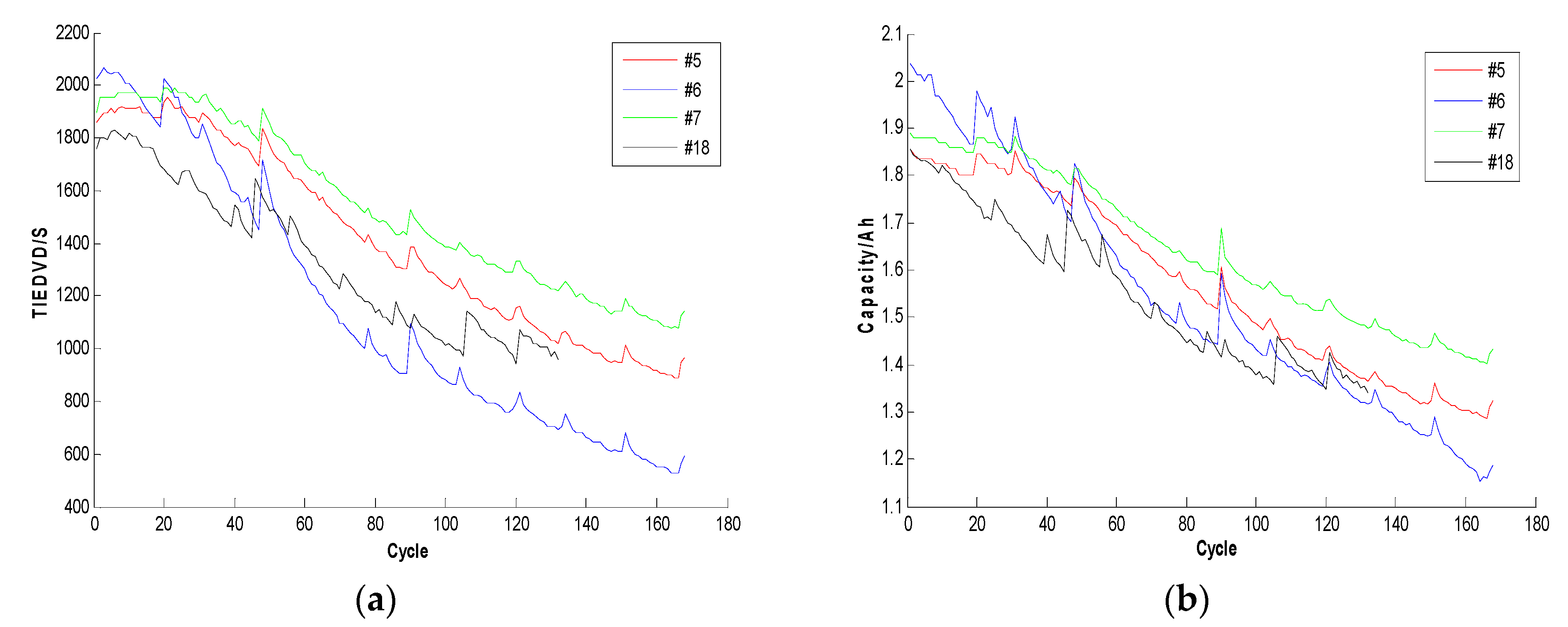
Using NASA’s battery #5, #6, #7, and #18, we have the extracted the HI series based on the three-step HI extraction procedure, as shown in Figure 2a. The batteries’ actual capacity degradation curve is shown in Figure 2b. We can see that there is similarity between the capacity degradation and the HI series.
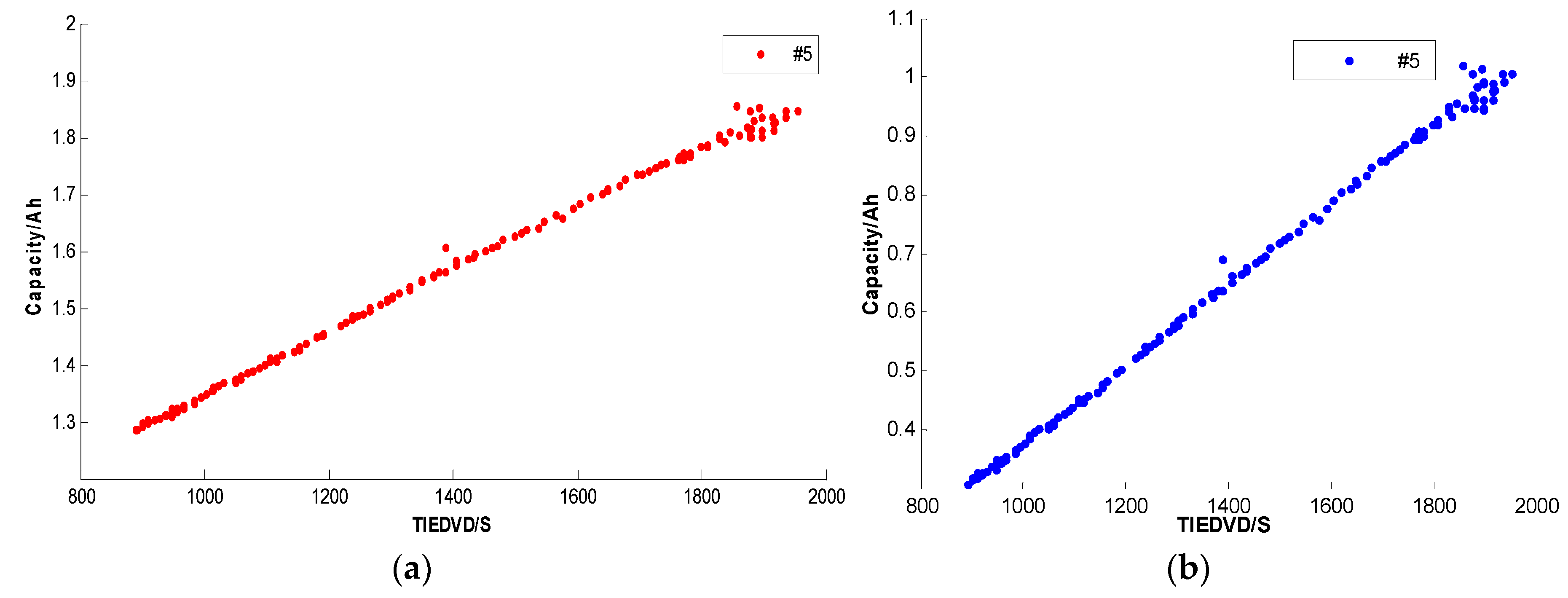
In this study, we only consider battery #5 to verify the on-line remaining useful life prediction method. Then, we use scatter plots to present the correlation between the TIEDVD and raw capacity series as shown in Figure 3. As can be seen, there is a close linear relationship between the HI series and battery capacity. However, there is still room for improvement of the linearity.
3.2. HI Optimization
3.2.1. Qualitative Analysis
In order to further improve the linearity of the extracted HI and battery capacity, the Box–Cox transformation is applied as introduced in Section 2.2.
With the identified parameter for the Box–Cox transformation, the linear model for the capacity (denoted C) and the TIEDVD is shown as:
where , , and is the transformed capacity as:
The logarithm is the natural logarithm (log base e). The algorithm calls for finding the λ value that maximizes the log-Likelihood Function (LLF). The search is conducted using Statistical Analysis System (SAS) software. We take the value λ from [−5, +5] at the interval 0.5. We choose the λ which maximizes g(λ). The correlation between the log-likelihood function and the parameter λ is shown in Figure 4. Thus, we choose λ = 1.5 to make the Box–Cox transformation. After the Box–Cox transformation, we get the correlation between transformed capacity and TIEDVD, as shown in Figure 3b. The linearity between the transformed capacity and the TIEDVD has been improved, but we need to further quantify the analysis.
3.2.2. Correlation Analysis and Evaluation
To quantitatively evaluate the improvement of the correlation after performing the Box–Cox transformation, the Pearson correlation and Spearman rank correlation between the TIDEVE series and capacity are calculated.
The Pearson correlation analysis is a measure of the linear dependence between the TIEDVD and the capacity. Pearson correlation coefficient r has a value between +1 and −1 inclusive, where 1 is total positive linear correlation, 0 is no linear correlation, and −1 is total negative linear correlation. The formula is as follows:
Spearman’s rank correlation analysis is a nonparametric measure of rank correlation. It assesses how well the relationship between two variables can be described using a monotonic function. While Pearson’s correlation assesses linear relationships, Spearman’s correlation assesses a monotonic relationship (whether linear or not). If there are no repeated data values, a perfect Spearman correlation of +1 or −1 occurs when each of the variables is a perfect monotone function of the other. It can be inferred that the Spearman correlation between the TIEDVD and capacity will be high. We use MATLAB to calculate the value of the Spearman rank correlation. Table 1 shows the correlation analysis results of battery #5.
In order to show the validity of the results in detail, the Spearman correlation coefficient is used to evaluate the linear relationship between the TIEDVD and the transformed capacity with different parameters λ. As shown in Figure 5, the Pearson correlation coefficient is at maximum at λ = 1.5, which verified the validity and rationality of the proposed maximum likelihood method. The highest Pearson correlation coefficients are 0.9988, approximating 1, which means that the transformed capacity and the TIEDVD have a very strong linear relationship. Although the Spearman correlation analysis shows that the relationship between transformed capacity and TIEDVD is not strictly monotonic, the TIEDVD is accurate enough to replace capacity through a linear function to be a new HI for quantifying battery degradation.
3.3. HI Performance Evaluation
3.3.1. Evaluation Criterion
The root mean squared error (RMSE) and the fitness degree () are two evaluation criteria to evaluate the performance of the extracted HI:
where C is the actual capacity, is the estimated capacity with transformation, is actual mean value of the C, and n is the sample size.
3.3.2. Evaluation Result
According to Equation (25), we can calculate , and then we can get the transformed capacity from . We can get the estimated capacity through Equation (21):
After all of the above computation, the detailed experimental results are shown in Figure 6 and Table 2.
We can see that the estimated capacity is very close to the actual capacity HI.
As shown in Table 2, is 0.9753 and RMSE is 0.0297, which means an adequate statistical fit. Both criteria indicate that the proposed method can provide an appropriate HI and improve the similarity between the extracted HI and capacity. Especially, the is almost equal to 1. Capacity can quantify the actual battery degradation, so the real-time degradation process can be effectively modeled with this extracted HI.
4. Battery RUL Prediction
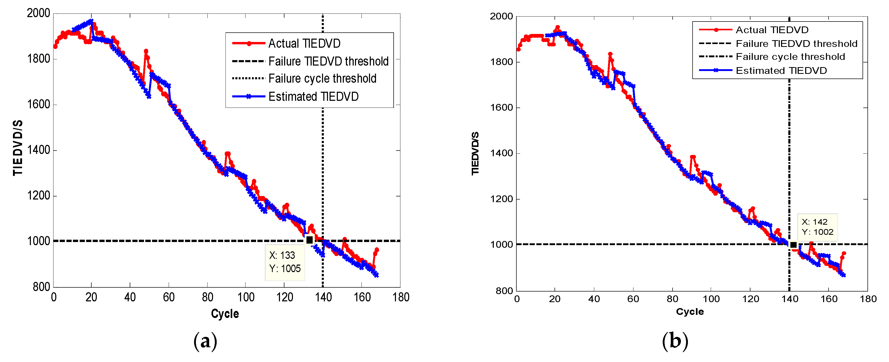
After the evaluation and verification of the extracted and optimized HI, we performed a RUL estimation with the optimized gray model GM(1,1). The RUL estimates are carried out at the starting points of 10th cycle, 15th cycle, and 20th cycle, respectively.
Before the prediction, we should calculate the failure TIEDVD threshold of the battery. As a fact, the end-of-life (EOL) criterion of the batteries is a 30% fade capacity rated from 2 Ahr to 1.4 Ahr. The Box–Cox transformed failure threshold capacity can be obtained. According to the linearity correlation between the transformed failure threshold capacity and the HI, we deduce the failure threshold of the TIEDVD. Battery #5’s failure threshold time was 1002 s, and the corresponding failure cycle was 140.
To evaluate the performance of RUL estimation, we use the absolute error (AE) and relative error (RE) defined by
where R is the actual RUL value, and are the predicted RUL values.
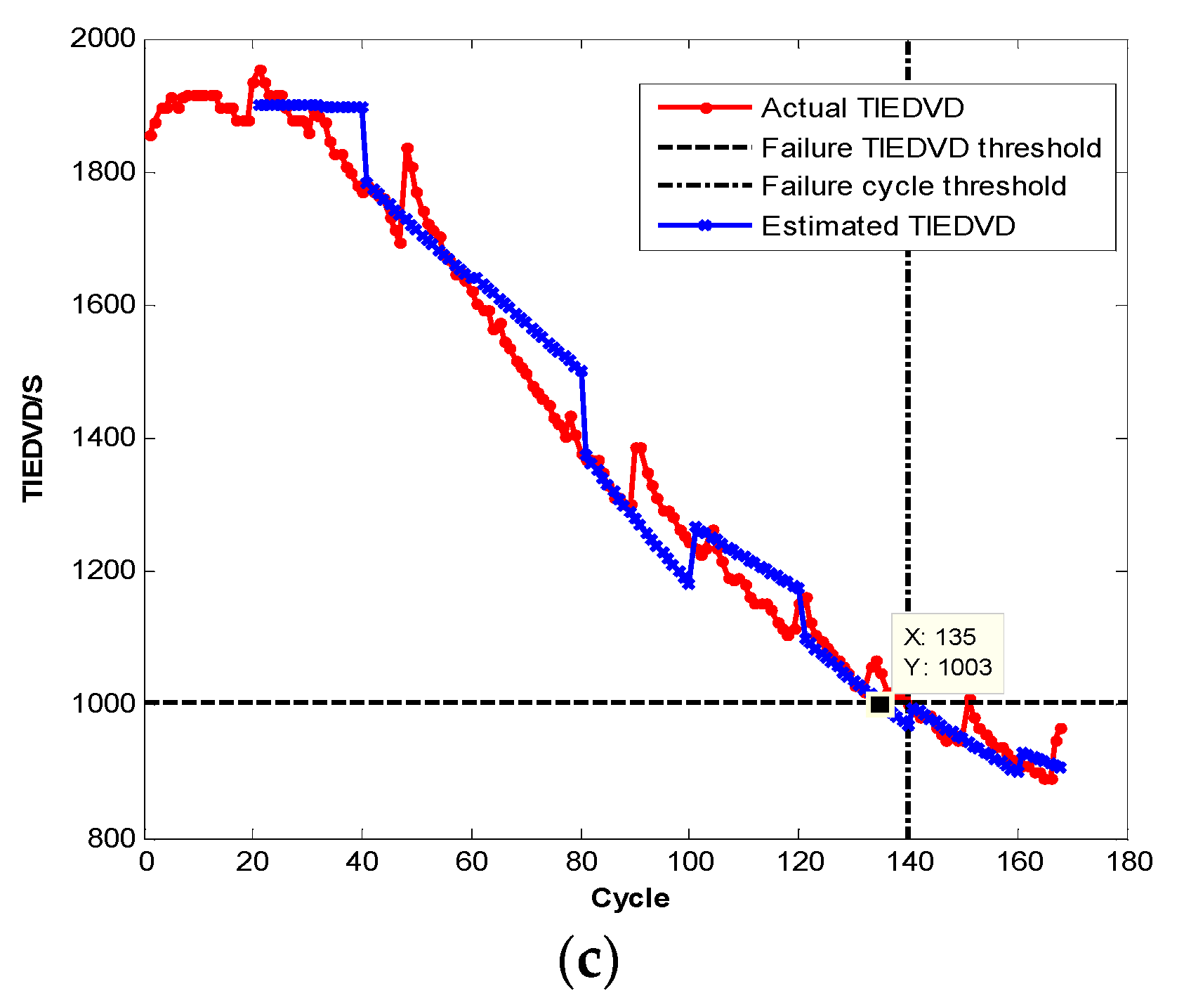
In order to verify the validity and accuracy of the proposed method, different iterative data points 10, 15, and 20 were used to predict the battery’s degradation process. The different iterative data points of the battery’s TIEDVD data sequence as the prediction began are used to build the optimized prediction model, when the old data is removed. Then a new data point is input to continue the prediction until the last data point has been utilized. The forecasting start points are 10, 15, and 20, respectively, which means the data points number i equals 10, 15, and 20, respectively, and the predicting number m equals 10, 20, and 5, respectively. The RUL prediction results are shown in Figure 8. As discussed in Section 2.2, the parameter a denotes the coefficient, which describes the fading trend of the testing samples, while the parameter b represents the influence of external impacts on TIEDVD fading. As we introduced the optimized gray model, the parameters a and b can self-adaptively change. These figures show that parameter a fluctuates over the cycle numbers and b decreases with cycle number, which indicates that the disturbance effect is restrained with the cycles. From Figure 8, the smaller the prediction number, the higher the accuracy of the prediction. The detailed numeric results are shown in Table 4.
5. Conclusions
In this paper, an optimized gray model is presented to predict the RUL of lithium-ion batteries by using the extracted HI from the discharge voltage and operating time. The optimized gray model has a strong dynamic adaptability, which is more robust and accurate, especially for small amounts of data and poor information. When comparing the HI with actual capacity, we find a linear correlation between the HI and capacity, which makes the HI as a lithium-ion battery degradation criterion more convincing. With the Box–Cox transformation, the HI is optimized to enhance the performance in the RUL’s estimation. The Pearson and Spearman correlation analyses are employed to assess the similarity between the real capacity and the estimated capacity derived from the HI. The results show that the prediction accuracy is satisfactory. Therefore, we can conclude that our proposed on-line prediction method is appropriate for quantifying lithium-ion battery degradation and making RUL predictions.
It is very meaningful to point out that the TIEDVD used in this paper is one in which the current is constant in each discharge cycle. Since the experimental data are obtained in a relatively stable environment, the degradation modes and cycle life features of batteries may be significantly different in practice.
In the future, we need to find more appropriate on-line HI for quantifying battery degradation and making RUL predictions. More importantly, lithium-ion battery degradation modeling and HI evaluation should be considered under different operating environments.
Author Contributions
Dong Zhou helped to guide many professional problems of English paper writing. Long Xue performed the data analysis and wrote the manuscript. Yijia Song contributed to analysis and manuscript preparation; Jiayu Chen revised the manuscript.
Conflicts of Interest
The authors declare no conflict of interest.
References
- Lithium-ion Battery. Available online: https://en.wikipedia.org/wiki/Lithium-ion_battery?wprov=sfla1 (accessed on 13 January 2001).
- Leng, F.; Tan, C.M.; Yazami, R.; Le, M.D. A practical framework of electrical based online state-of-charge estimation of lithium ion batteries. J. Power Sources 2014, 255, 423–430. [Google Scholar] [CrossRef]
- Williard, N.; He, W.; Hendricks, C.; Pecht, M. Lessons Learned from the 787 Dreamliner Issue on Lithium-Ion Battery Reliability. Energies 2013, 6, 4682–4695. [Google Scholar] [CrossRef]
- Rezvanizaniani, S.M.; Liu, Z.; Chen, Y.; Lee, J. Review and recent advances in battery health monitoring and prognostics technologies for electric vehicle (EV) safety and mobility. J. Power Sources 2014, 256, 110–124. [Google Scholar] [CrossRef]
- Tang, S.; Yu, C.; Wang, X.; Guo, X.; Si, X. Remaining Useful Life Prediction of Lithium-Ion Batteries Based on the Wiener Process with Measurement Error. Energies 2014, 7, 520–547. [Google Scholar] [CrossRef]
- Si, X.S.; Wang, W.; Hu, C.H.; Zhou, D.H. Remaining useful life estimation—A review on the statistical data driven approaches. Eur. J. Oper. Res. 2011, 213, 1–14. [Google Scholar] [CrossRef]
- Zhang, J.; Lee, J. A review on prognostics and health monitoring of Li-ion battery. J. Power Sources 2011, 196, 6007–6014. [Google Scholar] [CrossRef]
- He, Y.J.; Shen, J.N.; Shen, J.F.; Ma, Z.F. State of health estimation of lithium-ion batteries: A multiscale Gaussian process regression modeling approach. AIChE J. 2015, 61, 1589–1600. [Google Scholar] [CrossRef]
- Dalal, M.; Ma, J.; He, D. Lithium-ion battery life prognostic health management system using particle filtering framework. J. Risk Reliab. 2011, 225, 81–90. [Google Scholar] [CrossRef]
- Yu, J. State-of-Health Monitoring and Prediction of Lithium-Ion Battery Using Probabilistic Indication and State-Space Model. IEEE Trans. Instrum. Meas. 2015, 64, 2937–2949. [Google Scholar]
- Miao, Q.; Cui, H.; Xie, L.; Zhou, X. Remaining useful life prediction of the lithium-ion battery using particle filtering. J. Chongqing Univ. 2013, 36, 47–52. [Google Scholar]
- Long, B.; Xian, W.; Jiang, L.; Liu, Z. An improved autoregressive model by particle swarm optimization for prognostics of lithium-ion batteries. Microelectron. Reliab. 2013, 53, 821–831. [Google Scholar] [CrossRef]
- Charkhgard, M.; Farrokhi, M. State-of-Charge Estimation for Lithium-Ion Batteries Using Neural Networks and EKF. IEEE Trans. Ind. Electron. 2010, 57, 4178–4187. [Google Scholar] [CrossRef]
- Bai, G.; Wang, P.; Hu, C.; Pecht, M. A generic model-free approach for lithium-ion battery health management. Appl. Energy 2014, 135, 247–260. [Google Scholar] [CrossRef]
- Eddahech, A.; Briat, O.; Bertrand, N.; Delétage, J.Y.; Vinassa, J.M. Behavior and state-of-health monitoring of Li-ion batteries using impedance spectroscopy and recurrent neural networks. Int. J. Electr. Power Energy Syst. 2012, 42, 487–494. [Google Scholar] [CrossRef]
- Khelif, R.; Chebel-Morello, B.; Malinowski, S.; Laajili, E.; Fnaiech, F.; Zerhouni, N. Direct Remaining Useful Life Estimation Based on Support Vector Regression. IEEE Trans. Ind. Electron. 2016, 64, 2276–2285. [Google Scholar] [CrossRef]
- Dong, H.; Jin, X.; Lou, Y.; Wang, C. Lithium-ion battery state of health monitoring and remaining useful life prediction based on support vector regression-particle filter. J. Power Sources 2014, 271, 114–123. [Google Scholar] [CrossRef]
- Klass, V.; Behm, M.; Lindbergh, G. A support vector machine-based state-of-health estimation method for lithium-ion batteries under electric vehicle operation. J. Power Sources 2014, 270, 262–272. [Google Scholar] [CrossRef]
- Chen, X.Z.; Yu, J.S.; Tang, D.Y.; Wang, Y.X. Probabilistic Residual Life Prediction for Lithium-ion Batteries Based on Bayesian LS-SVR. Acta Aeronaut. Astronaut. Sin. 2013, 34, 2219–2229. [Google Scholar]
- Wang, S.; Zhao, L.; Su, X.; Ma, P. Prognostics of Lithium-Ion Batteries Based on Battery Performance Analysis and Flexible Support Vector Regression. Energies 2014, 7, 6492–6508. [Google Scholar] [CrossRef]
- Saha, B.; Goebel, K.; Christophersen, J. Comparison of prognostic algorithms for estimating remaining useful life of batteries. Trans. Inst. Meas. Control 2009, 31, 293–308. [Google Scholar] [CrossRef]
- Rezvani, M.; Lee, S.; Lee, J. A Comparative Analysis of Techniques for Electric Vehicle Battery Prognostics and Health Management (PHM); Society of Automotive Engineers (SAE) International: Warrendale, PA, USA, 2011. [Google Scholar]
- Arabmakki, E.; Kantardzic, M.; Sethi, T.S. RLS-A reduced labeled samples approach for streaming imbalanced data with concept drift. In Proceedings of the 2014 IEEE 15th International Conference on Information Reuse and Integration, San Francisco, CA, USA, 13–15 August 2014; pp. 779–786. [Google Scholar]
- Liu, J.; Wang, W.; Ma, F.; Yang, Y.B.; Yang, C.S. A data-model-fusion prognostic framework for dynamic system state forecasting. Eng. Appl. Artif. Intell. 2012, 25, 814–823. [Google Scholar] [CrossRef]
- Liu, D.; Luo, Y.; Liu, J.; Peng, Y.; Guo, L.; Pecht, M. Lithium-ion battery remaining useful life estimation based on fusion nonlinear degradation AR model and RPF algorithm. Neural Comput. Appl. 2014, 25, 557–572. [Google Scholar] [CrossRef]
- Kozlowski, J.D. Electrochemical cell prognostics using online impedance measurements and model-based data fusion techniques. In Proceedings of the 2003 IEEE Aerospace Conference, Big Sky, MT, USA, 8–15 March 2003; pp. 3257–3270. [Google Scholar]
- Li, F.; Xu, J. A new prognostics method for state of health estimation of lithium-ion batteries based on a mixture of Gaussian process models and particle filter. Microelectron. Reliab. 2015, 55, 1035–1045. [Google Scholar] [CrossRef]
- Xing, Y.; Ma, E.W.M.; Tsui, K.L.; Pecht, M. An ensemble model for predicting the remaining useful performance of lithium-ion batteries. Microelectron. Reliab. 2013, 53, 811–820. [Google Scholar] [CrossRef]
- Chiang, Y.-H.; Sean, W.-Y.; Ke, J.-C. Online estimation of internal resistance and open-circuit voltage of lithium-ion batteries in electric vehicles. J. Power Sources 2011, 196, 3921–3932. [Google Scholar] [CrossRef]
- Liu, D.; Zhou, J.; Liao, H.; Peng, Y.; Peng, X. A Health Indicator Extraction and Optimization Framework for Lithium-Ion Battery Degradation Modeling and Prognostics. IEEE Trans. Syst. Man Cybern. Syst. 2015, 45, 915–928. [Google Scholar]
- Widodo, A.; Shim, M.C.; Caesarendra, W.; Yang, B.S. Intelligent prognostics for battery health monitoring based on sample entropy. Expert Syst. Appl. Int. J. 2011, 38, 11763–11769. [Google Scholar] [CrossRef]
- Shahriari, M.; Farrokhi, M. Online State-of-Health Estimation of VRLA Batteries Using State of Charge. IEEE Trans. Ind. Electron. 2013, 60, 191–202. [Google Scholar] [CrossRef]
- Williard, N.; He, W.; Osterman, M.; Pecht, M. Comparative Analysis of Features for Determining State of Health in Lithium-Ion Batteries. Int. J. Progn. Health Manag. 2013, 4, 1–7. [Google Scholar]
- Zhou, Y.; Huang, M.; Chen, Y.; Tao, Y. A novel health indicator for on-line lithium-ion batteries remaining useful life prediction. J. Power Sources 2016, 321, 1–10. [Google Scholar] [CrossRef]
- Liu, D.; Wang, H.; Peng, Y.; Xie, W.; Liao, H. Satellite Lithium-Ion Battery Remaining Cycle Life Prediction with Novel Indirect Health Indicator Extraction. Energies 2013, 6, 3654–3668. [Google Scholar] [CrossRef]
- Lu, I.J.; Lin, S.J.; Lewis, C. Grey relation analysis of motor vehicular energy consumption in Taiwan. Energy Policy 2008, 36, 2556–2561. [Google Scholar] [CrossRef]
- Kayacan, E.; Ulutas, B.; Kaynak, O. Grey System Theory-Based Models in Time Series Prediction. Expert Syst. Appl. 2010, 37, 1784–1789. [Google Scholar] [CrossRef]
- Xu, J.; Tan, T.; Tu, M.; Qi, L. Improvement of grey models by least squares. Expert Syst. Appl. 2011, 38, 13961–13966. [Google Scholar] [CrossRef]
- Chen, L.; Lin, W.; Li, J.; Tian, B.; Pan, H. Prediction of lithium-ion battery capacity with metabolic grey model. Energy 2016, 106, 662–672. [Google Scholar] [CrossRef]
- Sakia, R.M. The Box-Cox Transformation Technique:A Review. J.R.Stat. Soc.B 1992, 41, 169–178. [Google Scholar]
- Saha, B.; Goebel, K. Battery Data Set, NASA Ames Prognostics Data Repository; NASA Ames Research Center: Moffett Field, CA, USA, 2007. Available online: http://ti.arc.nasa.gov/project/prognostic-data-repository (accessed on 26 October 2010).
Figure 1.
Health indicator (HI) extraction with time interval and discharging voltage difference.
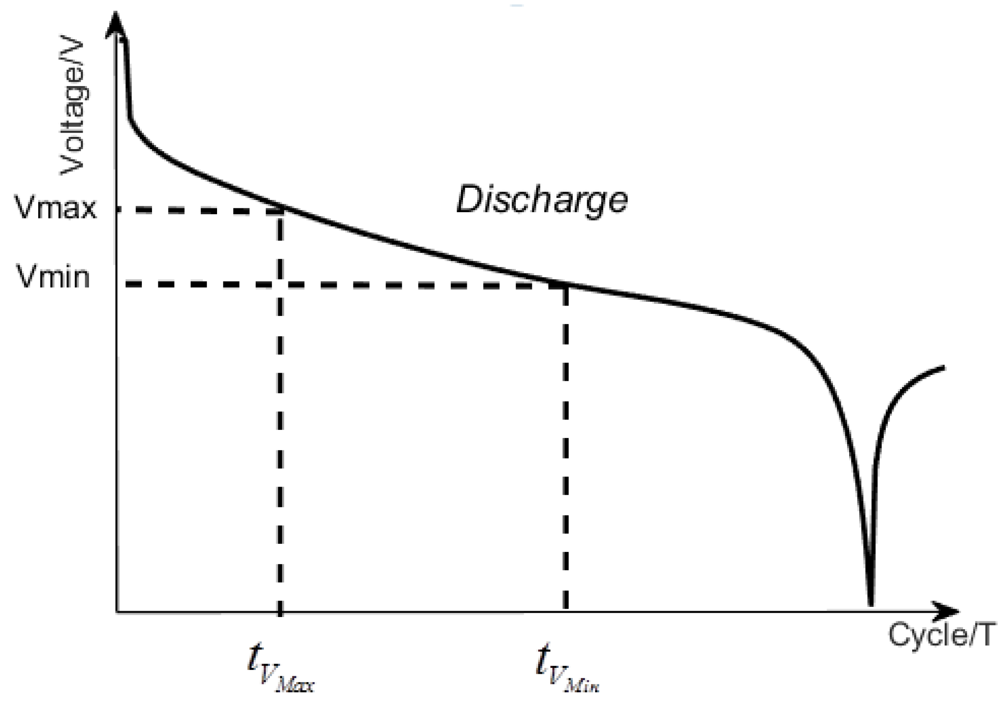
Figure 2.
National Aeronautics and Space Administration (NASA) battery degradation curve of extracted HI and capacity. (a) The extracted HI, time interval of equal discharging voltage difference (TIEDVD) degradation curve; (b) The actual capacity degradation curve.
Figure 2.
National Aeronautics and Space Administration (NASA) battery degradation curve of extracted HI and capacity. (a) The extracted HI, time interval of equal discharging voltage difference (TIEDVD) degradation curve; (b) The actual capacity degradation curve.

Figure 3.
Liner correlation between TIEDVD and capacity. (a) The linear correlation between TIEDVD and raw capacity; (b) The linear correlation between TIEDVD and transformed capacity.
Figure 3.
Liner correlation between TIEDVD and capacity. (a) The linear correlation between TIEDVD and raw capacity; (b) The linear correlation between TIEDVD and transformed capacity.

Figure 4.
Log-likelihood function with parameter λ.
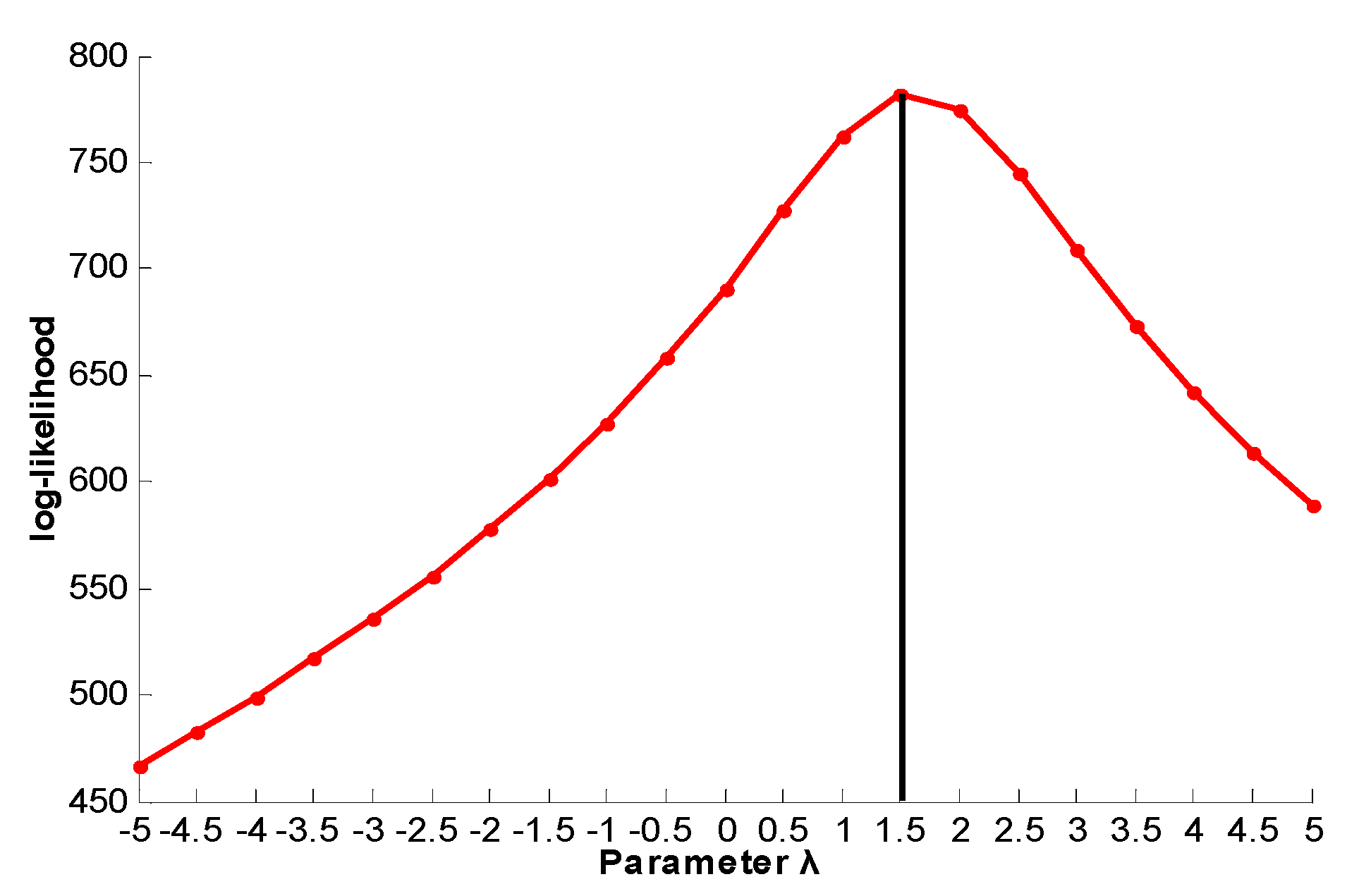
Figure 5.
Pearson correlation coefficient with parameter λ.
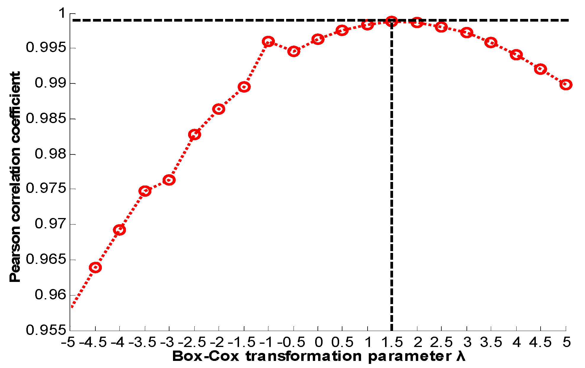
Figure 6.
Actual capacity and estimated capacity (battery #5).
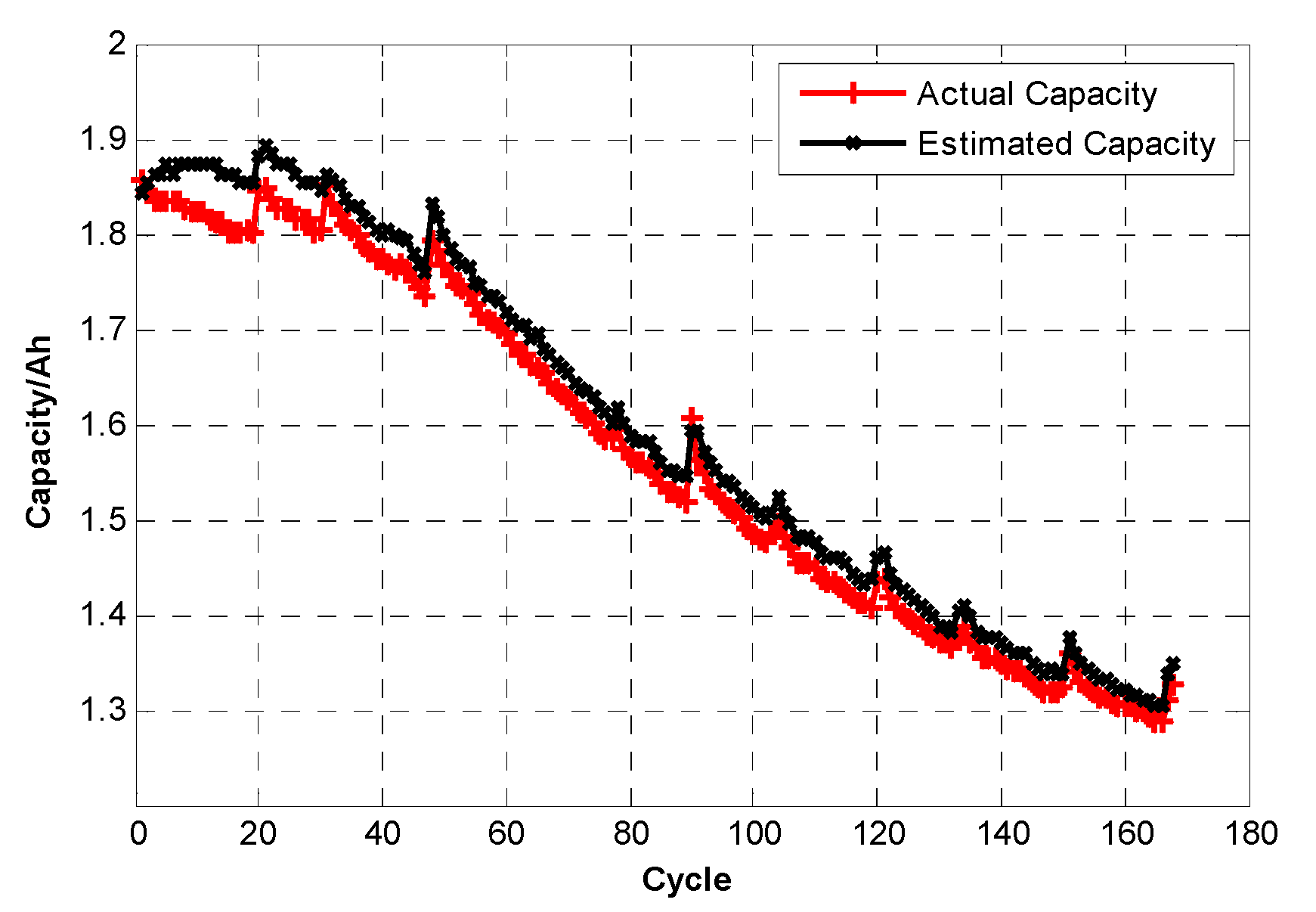
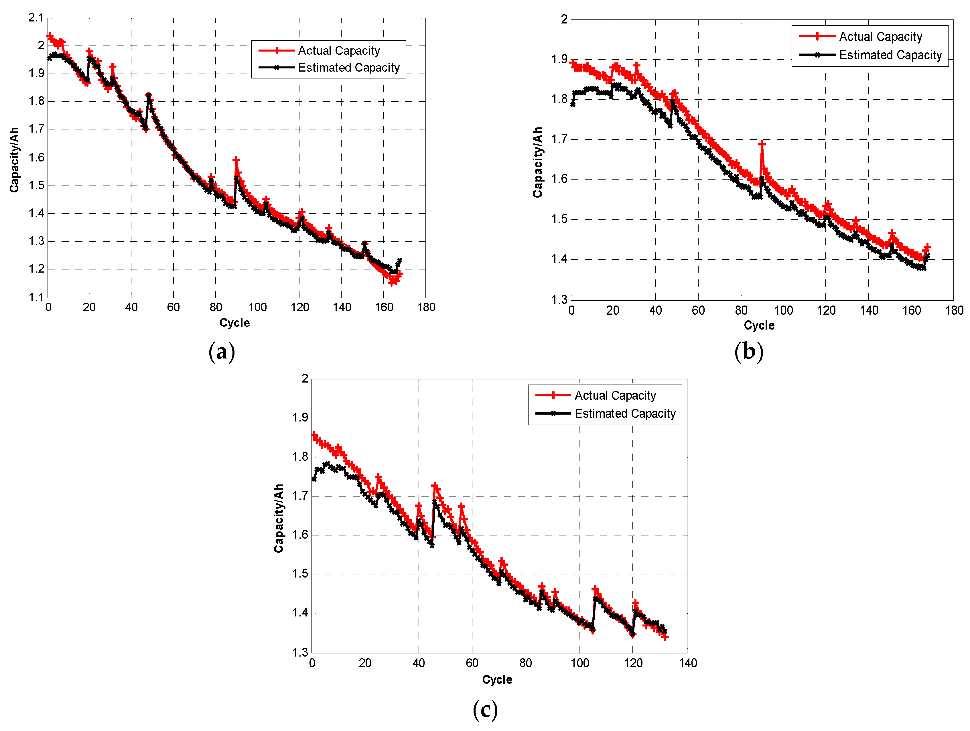
Figure 7.
HI for various lithium-ion batteries capacity estimated. HI for lithium-ion battery with (a) #6; (b) #7; (c) #18.
Figure 7.
HI for various lithium-ion batteries capacity estimated. HI for lithium-ion battery with (a) #6; (b) #7; (c) #18.

Figure 8.
RUL prediction with TIEDVD at (a) 10 cycles; (b) 15 cycles; (c) 20 cycles. The forecasting numbers are 10, 5, and 20, respectively.
Figure 8.
RUL prediction with TIEDVD at (a) 10 cycles; (b) 15 cycles; (c) 20 cycles. The forecasting numbers are 10, 5, and 20, respectively.

Table 1.
Correlation analysis.
| Time | Pearson Correlation | Spearman Rank Correlation |
|---|---|---|
| Before Box–Cox transformation | 0.9984 | 0.9937 |
| After Box–Cox transformation | 0.9988 | 0.9937 |
Table 2.
HI performance evaluation results.
| λ | RSEM | R2 |
|---|---|---|
| 1.5 | 0.0297 | 0.9753 |
Table 3.
HI evaluated results of other three NASA lithium-ion batteries.
| Index | λ | RSEM | R2 |
|---|---|---|---|
| #6 | 2.0 | 0.0200 | 0.9937 |
| #7 | 1.0 | 0.0379 | 0.9384 |
| #18 | 0.5 | 0.0273 | 0.9686 |
Table 4.
Remaining useful life (RUL) prediction results.
| Starting Point | Prediction Number | RUL | Predicted RUL | AE | RE |
|---|---|---|---|---|---|
| 10 | 10 | 130 | 123 | 7 | 5.38% |
| 15 | 20 | 125 | 115 | 10 | 8.00% |
| 20 | 5 | 120 | 122 | 2 | 1.67% |
© 2017 by the authors. Licensee MDPI, Basel, Switzerland. This article is an open access article distributed under the terms and conditions of the Creative Commons Attribution (CC BY) license (http://creativecommons.org/licenses/by/4.0/).
Share and Cite
MDPI and ACS Style
Zhou, D.; Xue, L.; Song, Y.; Chen, J. On-Line Remaining Useful Life Prediction of Lithium-Ion Batteries Based on the Optimized Gray Model GM(1,1). Batteries 2017, 3, 21. https://doi.org/10.3390/batteries3030021
AMA Style
Zhou D, Xue L, Song Y, Chen J. On-Line Remaining Useful Life Prediction of Lithium-Ion Batteries Based on the Optimized Gray Model GM(1,1). Batteries. 2017; 3(3):21. https://doi.org/10.3390/batteries3030021
Chicago/Turabian StyleZhou, Dong, Long Xue, Yijia Song, and Jiayu Chen. 2017. "On-Line Remaining Useful Life Prediction of Lithium-Ion Batteries Based on the Optimized Gray Model GM(1,1)" Batteries 3, no. 3: 21. https://doi.org/10.3390/batteries3030021
Note that from the first issue of 2016, this journal uses article numbers instead of page numbers. See further details here.