Article

3D Reconstruction of Plant/Tree Canopy Using Monocular and Binocular Vision

Department of Agricultural & Biological Engineering, University of Florida, Gainesville, FL 32611, USA
*
Author to whom correspondence should be addressed.
J. Imaging 2016, 2(4), 28; https://doi.org/10.3390/jimaging2040028
Submission received: 29 August 2016 / Revised: 16 September 2016 / Accepted: 19 September 2016 / Published: 29 September 2016
(This article belongs to the Special Issue Image Processing in Agriculture and Forestry)

Abstract

:
Three-dimensional (3D) reconstruction of a tree canopy is an important step in order to measure canopy geometry, such as height, width, volume, and leaf cover area. In this research, binocular stereo vision was used to recover the 3D information of the canopy. Multiple images were taken from different views around the target. The Structure-from-motion (SfM) method was employed to recover the camera calibration matrix for each image, and the corresponding 3D coordinates of the feature points were calculated and used to recover the camera calibration matrix. Through this method, a sparse projective reconstruction of the target was realized. Subsequently, a ball pivoting algorithm was used to do surface modeling to realize dense reconstruction. Finally, this dense reconstruction was transformed to metric reconstruction through ground truth points which were obtained from camera calibration of binocular stereo cameras. Four experiments were completed, one for a known geometric box, and the other three were: a croton plant with big leaves and salient features, a jalapeno pepper plant with median leaves, and a lemon tree with small leaves. A whole-view reconstruction of each target was realized. The comparison of the reconstructed box’s size with the real box’s size shows that the 3D reconstruction is in metric reconstruction.

1. Introduction

Three-dimensional (3D) reconstruction of a plant/tree canopy can not only be used to measure the height, width, volume, area, and biomass of the target, but also can be used to visualize the object in virtual 3D space. 3D reconstruction is also called 3D digitizing or 3D modeling. Plant/tree 3D reconstruction could be cataloged into two types: (1) depth-based 3D modeling; and (2) image-based 3D modeling. Depth-based 3D modeling involves using sensors, such as, ultrasonic sensors, lasers, Time-of-Flight (ToF) cameras, and Microsoft red, green, and blue depth (RGB-D) cameras.
Using ultrasonic sensors, Sinoquet et al. [1] created a 3D model of corn plant profiles and canopy structure. The 3D results were used to calculate the leaf area and its distribution in the plant. Tumbo et al. [2] used ultrasonics in the field to measure citrus canopy volume. Twenty ultrasonic transducers were arranged on vertical boards (10 sensors per side). The ultrasonic sensors were installed behind a tractor, which was assumed to travel at an approximate speed of 0.5 km/h. A formula was provided to calculate the volume. To study the accuracy of this calculation, Zaman and Salyani [3] conducted research on the effect of ground speed and foliage density on canopy volume measurement. The experimental results showed that there was a 17.37% to 28.71% difference between the estimated and manually measured volumes.
Also using laser sensors, Tumbo et al. [2] described how to measure citrus canopy volume. Comparisons were made between the estimated volume and manually measured volume. The results showed high correlation. Wei and Salyani [4] employed a laser scanner and developed a laser scanning system, data acquisition system, and corresponding algorithm to calculate tree height, width, and canopy volume. To evaluate the accuracy of their system, a rectangular box was used as a target. Five repeated experiments were conducted to measure the box’s height, length, and volume. However, no direct comparison between estimated volume and manually measured volume of citrus trees was made. Wei and Salyani [5] extended the same laser scanning system to calculate foliage density. They defined foliage density as the ratio of foliage volume to tree canopy volume, where foliage volume was defined as the space contained within the laser incident points and the tree row plane, while canopy volume was defined as the space enclosed between outer canopy boundary and the tree row plane. Lee and Ehsani [6] developed a laser scanner-based system to measure citrus geometric characteristics. After the experimental trees were trimmed to an ellipsoid shape, whose volumes were easy to manually measure, the surface area and volume were estimated by using a laser scanner. Rosell et al. [7] reported the use of a 2D light detection and ranging (LIDAR) scanner to obtain the 3D structures of plants. Sanz-Cortiella et al. [8] assumed that there was a linear relationship between the tree leaf area and the number of impacts of laser beam on the target. The point clouds generated by the laser scanner were used to calculate the total leaf area. Both indoor and outdoor experiments were conducted to validate this assumption. Zhu et al. [9] reconstructed the shape of a tree crown from scanned data-based on alpha shape modeling. A boundary mesh model was extracted from the boundary point cloud. This method resulted in a rough shape reconstruction of a big (20-meter high) tree.
Studying the application of a ToF camera, Cui et al. [10] described a 3D reconstruction method initiated by scanning the object using the ToF camera, and the reconstruction was realized through the combination of 3D super-resolution and a probabilistic multiple scan alignment algorithm. In 3D reconstruction, a ToF camera was usually used in combination with a red, green, and blue (RGB) camera. The ToF camera provided depth information, and the RGB camera would give color information. Shim et al. [11] presented a method to calibrate a multiple view acquisition system composed of ToF cameras and RGB color cameras. This system has the ability to calibrate multi-modal sensors in real time. Song et al. [12] combined a ToF image with images taken from stereo cameras to estimate a depth map for plant phenotyping. The experiments were conducted in a glasshouse using green pepper plants as targets. The canopy characteristics such as stem length, leaf area, and fruit size were estimated. This estimation was a challenging task since occlusion was occuring. The depth information from the ToF image was used to assist the determination of the disparity between left and right images. A global optimization method, using graph cuts developed by Boykov and Kolmogorov [13], was also used to find the disparity. The result using the graph cuts (GC) method was compared with the one resulting from combing graph cuts and ToF depth information. A quality evaluation was conducted, and GC + ToF gave the highest score. A smooth surface reconstruction of a pepper leaf was obtained using this method. Adhikari and Karkee [14] developed a 3D vision system to automatically prune apple trees. The vision system was composed of a ToF 3D camera and a RGB color camera. Experimental results showed that this system had about 90% accuracy in identifying pruning points.
The RGB-D camera is a Microsoft [15] product called Kinect that is designed for Xbox360. Kinect is composed of a RGB camera, a depth camera, and an infrared laser projector. Kinect was mostly used indoors for video game and view reconstruction. Izadi et al. [16] and Newcombe et al. [17] used a moving Kinect to reconstruct a dense indoor view. Kinect Fusion was employed to realize the reconstruction in real time because there was a special requirement on their hardware, specifically the GPU, to use it. Chene et al. [18] applied Kinect on 3D phenotyping of plants. An algorithm was developed to segment the depth image from the top view of the plant. The 3D view of the plant was then reconstructed from the segmented depth image. Azzari et al. [19] used Kinect to characterize vegetation structure. The measurements calculated from their depth image matched well with the results of a plant size measured manually. Different experiments were conducted in the lab, and in an outdoor field under different light conditions—such as early afternoon, late afternoon, and night. Experimental results showed that the Kinect had a limitation under direct sunlight. Wang and Zhang [20] used two Kinect devices to make a 3D reconstruction of a dormant cherry tree that was moved into a laboratory environment. During the experiment, some parts of the branches were missed due to occlusion and a long distance between camera and tree. The reconstructed results could be used for automatic pruning.
Image-based 3D modeling involved reconstructing the 3D properties from 2D images by using single camera or stereo cameras. Zhang et al. [21] used stereo vision to reconstruct a 3D corn model. The boundaries of the corn leaves were extracted and matched. The 3D leaves were modeled using a space intersection algorithm from 2D boundaries. This was a two-image reconstruction. Song [22] used stereo vision to model crops in horticulture. The cameras were installed on the top of the crops, and a top view of the crop was reconstructed. Han and Burks [23] did work on 3D reconstruction of a citrus canopy. Multiple images were used, and consecutive images were stitched together through image mosaic techniques. The canopy was reconstructed from the stitched image. The results did not realize real-size reconstruction.
The estimation of camera matrices is the first step in 3D reconstruction. The method of self-calibration described by Pollefeys et al. [24,25] is usually used. Fitzgibbon and Zisserman [26] described a method to automatically recover camera matrices and 3D scene points from a sequence of images. These images were sequentially acquired through an uncalibrated camera, and image triplets were used to estimate camera matrices and 3D points. Then the consecutive image triplets were formed into a sequence through one-view overlapping or two-view overlapping. Snavely et al. [27] developed a novel method to recover camera matrices and 3D points from unordered images. All these technologies were known as Structure from Motion (SfM). The sparse feature points were used to match the images. The most often used features were called Scale Invariant Feature Transform (SIFT) as described by Lowe [28].
Quan et al. [29] did research on plant modeling based on multiple images. SfM was used to estimate camera motion from multiple images. Here, instead of using sparse feature points, quasi-dense feature points as described by Lhuillier and Quan [30] were used to estimate camera matrices and 3D points of the plant. The leaves of the plant were modeled by segmenting the 2D images and computing the depths using the computed 3D points, and the branches were drawn through an interactive procedure. This modeling method was suitable for a plant with distinguishable leaves. To model a tree, which has small leaves, Tan et al. [31] did research on image-based 3D reconstruction. SfM was also employed to recover camera matrices and 3D quasi-dense points. To make a full 3D reconstruction of the tree, the visible branches were first reconstructed, followed by the occluded branches. The occluded branches were reconstructed through an unconstrained growth and constrained growth method. Subsequently, the leaves were added to the branches. Some of the leaves were from segmented images, while others were derived from the synthesizing methodology. Teng et al. [32] used machine vision to recover the sparse and unoccluded leaves in three dimensions. The method used was similar to the work of Quan et al. [29]. The results of the 3D reconstruction were used to classify the leaves and to identify the plant’s type.
Furukawa and Ponce [33] provided a patch-based multiple view stereo (PMVS) algorithm to produce dense points to model the target. Small rectangular patches, called surfel, were used as feature points. The cameras’ matrices were pre-calibrated using the method provided by Snavely et al. [27]. Features in each image were detected, then matched across multiple images. An expansion procedure, similar to the method provided by Lhuillier and Quan [30], was used to produce a denser set of patches.
Santos and Oliveira [34] applied the PMVS method to agricultural crops, such as basil and ixora. Plants with big and unoccluded leaves were well reconstructed. The reported processing time for 143 basil images was approximately 110 min, and almost 40 min for 77 ixora images. The image numbers will increase with the plant’s size, consequently the processing time required will also increase with the increased number of images. Most of the processing was spent on feature detection and matching. The matching procedure was conducted through serial computation; however, if it could be conducted in parallel computation, the processing time would be significantly reduced. Currently, a Graphics processing unit (GPU)-based SIFT, which is known as SiftGPU described by Wu [35], is available to do key points detection and matching via parallel computing. The bundler package described by Snavely [36] and the PMVS package developed by Furukawa and Ponce [33] were combined into a single package called VisualSFM by Wu [37], which involved using parallel computing technology. This would significantly decrease the running time.
The objectives of our study were to:
  • Provide a new method to calibrate camera calibration matrix in metric level.
  • Apply the fast software ‘VisualSFM’ on complicate objects, e.g., plant/tree, to generate a full-view 3D reconstruction.
  • Generate the metric 3D reconstruction from projective reconstruction and achieve real-size 3D reconstruction for complicate agricultural plant scenes.

2. Materials and Methods
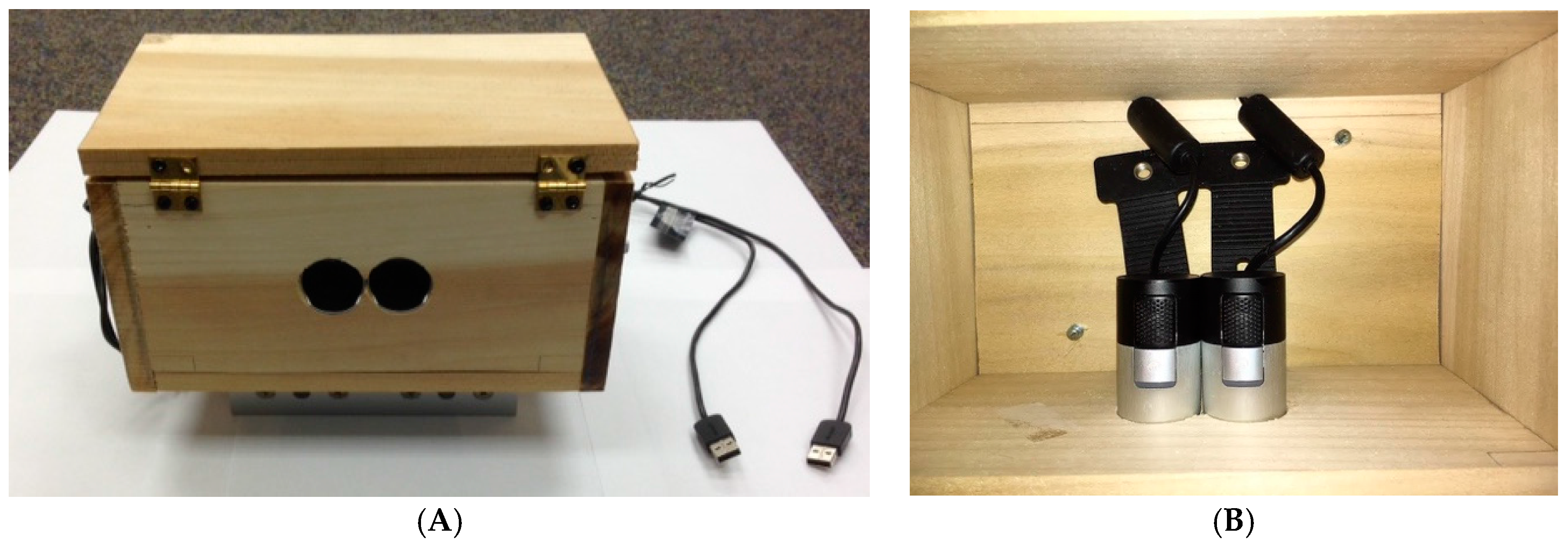
2.1. Hardware

In this paper, two Microsoft LifeCam Studio web high definition (HD) cameras (1080 p) were assembled inside a wooden box, and mounted approximately in parallel, with the baseline at 30 mm, as shown in Figure 1. To acquire images, they were connected to a Lenovo IdeaPad Y500 laptop with a NVIDIA GeForce GT650M GPU, which can be used in parallel computation to accelerate the computing time in feature points detection and matching.

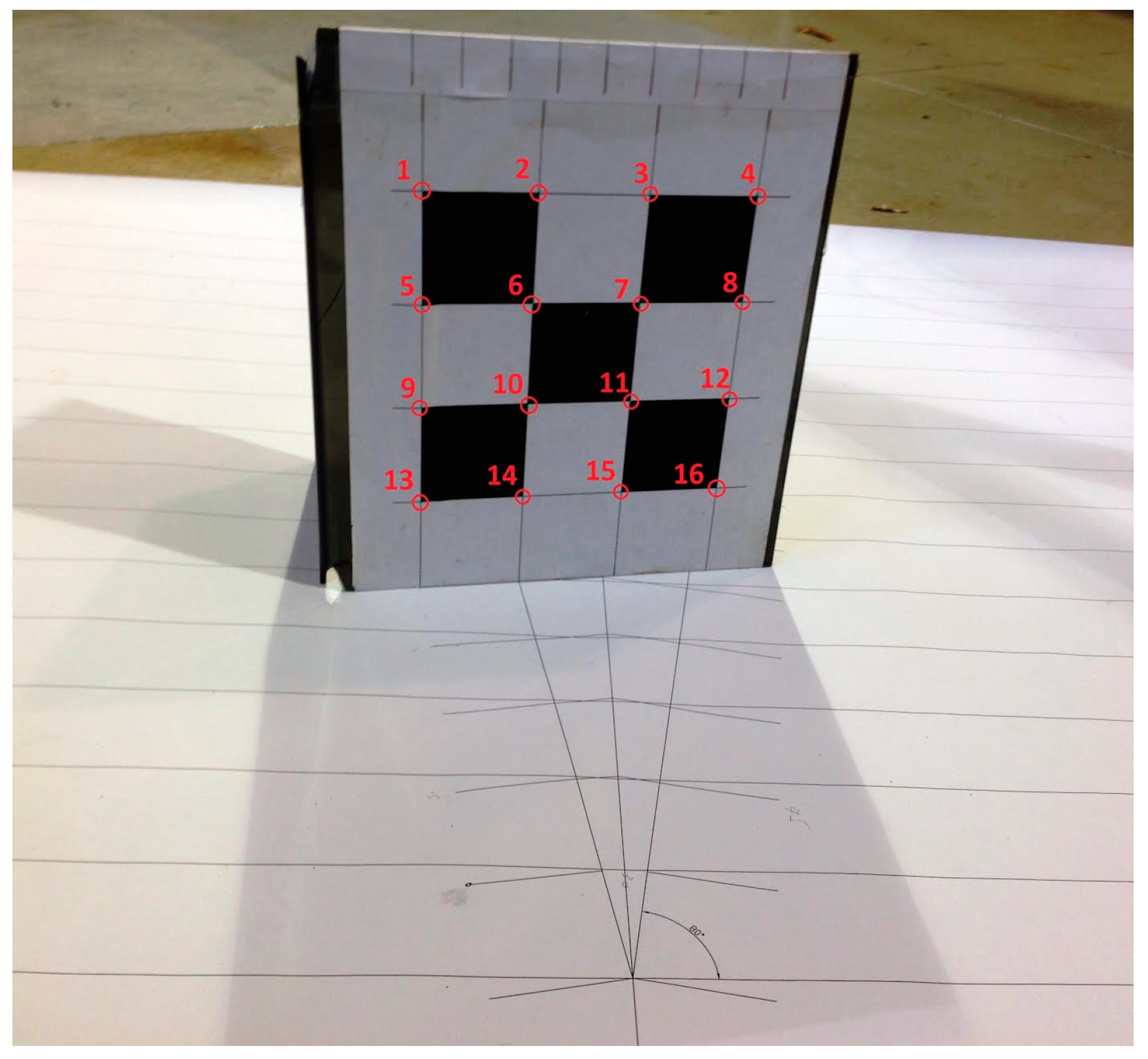
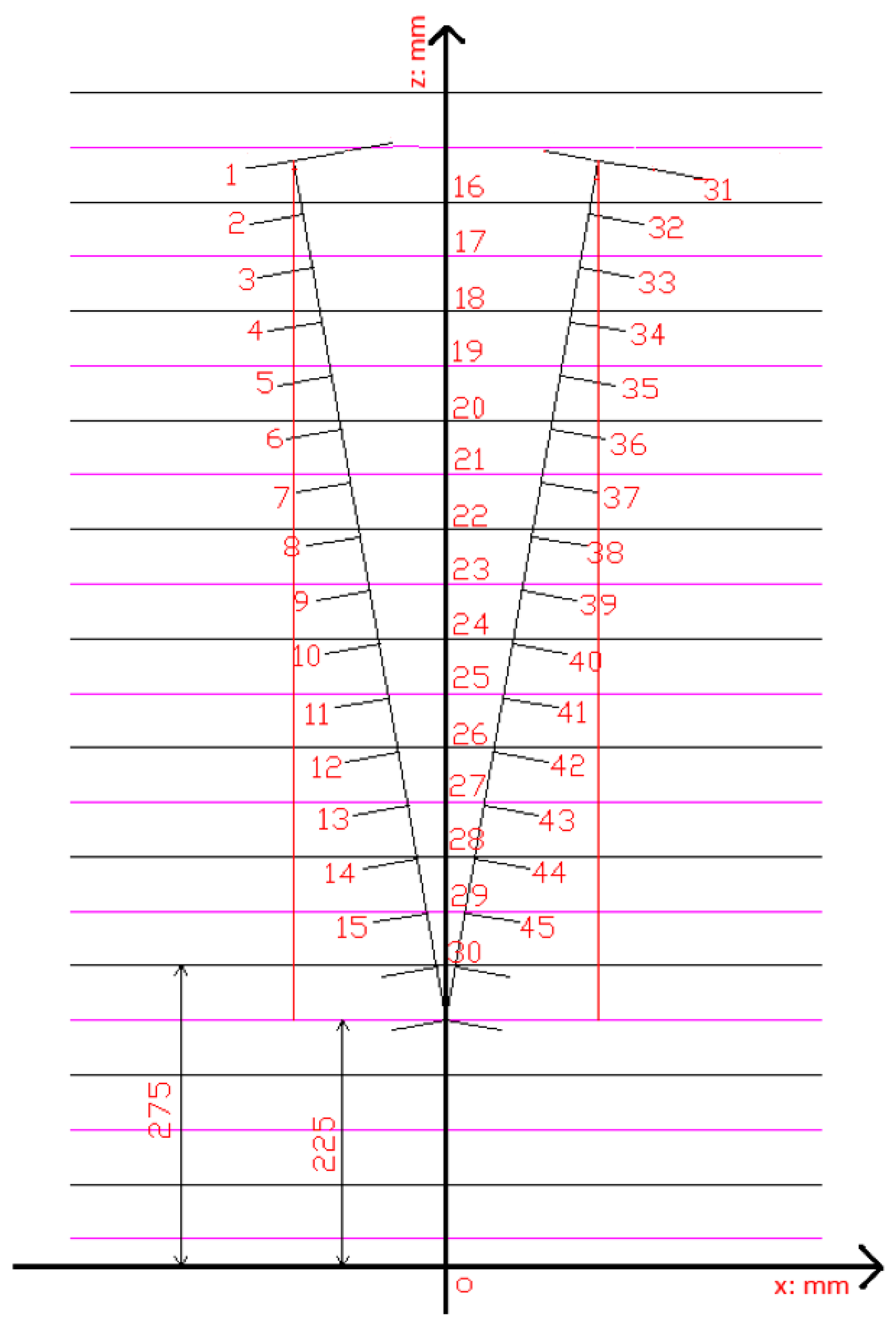
2.2. Stereo Camera Calibration

A 3D point ( X ) and its projection ( x ) in 2D image is related through camera calibration matrix P. The relationship is expressed as s x = P X , where x = ( x , y , 1 ) T is in homogenous form in 2D, X = ( X , Y , Z , 1 ) T is in homogenous form in 3D, P is a 3 × 4 matrix, and s is a scale. The objective of camera calibration is to determine camera calibration matrix P, which includes both intrinsic parameters and extrinsic parameters. Zhang [38] provided a flexible technique for camera calibration using only five images taken from different angles. A checkerboard was used as calibration pattern. For each image, the plane of the checkerboard was assumed as z-plane, so the Z coordinates for all the 3D points were zero. X and Y coordinates could be obtained from the actual checkerboard size. All these provided ground truth. A Matlab toolbox, developed by Bouguet [39], was used to solve camera calibration matrix using Zhang’s algorithm. This toolbox is not only suitable for a single camera, but is also suitable for stereo cameras.
The external camera parameters provided by Zhang’s [38] method were built on each checkerboard’s own coordinate system, not on the same world coordinate system. In order to build the same world coordinate system, a large 2D x-z coordinate system was plotted on an A0-size paper, together with a vertical checkerboard (Figure 2), and all of these provided the 3D ground truth on the same coordinate system. The detailed 2D x-z coordinate system is shown in Figure 3. Each line in the x-z plane was at 50 mm spacing. The middle line (oz) was rotated −10° around Oorig to get the left line, and rotated +10° around Oorig to get the right line. The checkerboard was then placed at different locations on the left, middle, and right line (marked as 1 through 45 in Figure 3). The 3D coordinates of each corner on the checkerboard, at each location, could be solved as the ground truth. Two images were taken at each location from the left and right cameras. From these 2D images, the 2D projection of these corners could also be solved.
Based on these 2D and 3D coordinates, the gold standard algorithm of Hartley and Zisserman [40] was used to calculate the camera matrices for both left and right cameras.
Based on camera calibration matrix and 2D image coordinates, we can get estimated 3D points. When compared to the actual 3D points, we can estimate the error in X, Y, and Z directions (Figure 4). These experimental results showed that this stereo camera set had good accuracy when the distance between cameras and the target was less than 800 mm. The statistical analysis for errors in the X, Y, and Z directions are shown in Table 1. The mean error in x direction is 0.42 mm, the mean error in y direction is 0.36 mm, and the mean error in z direction is 2.78 mm.

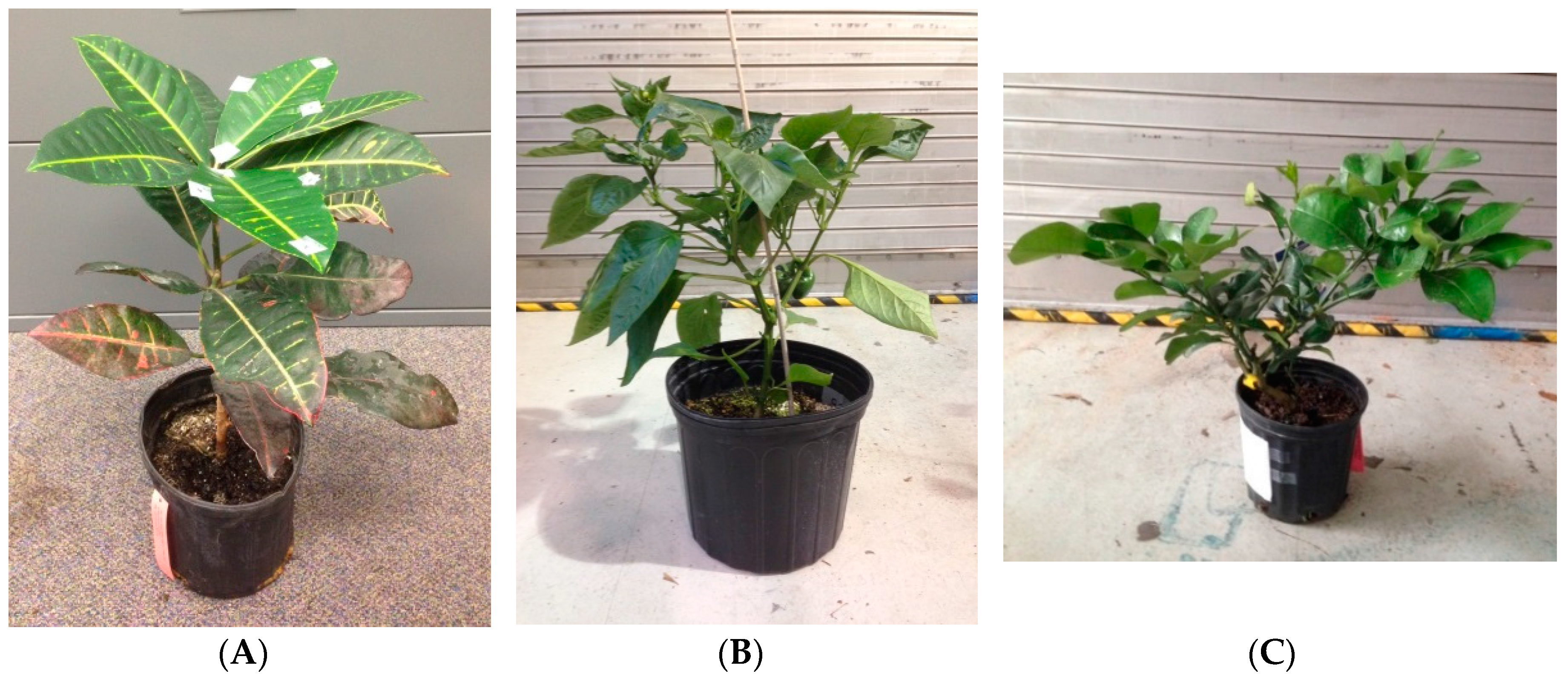
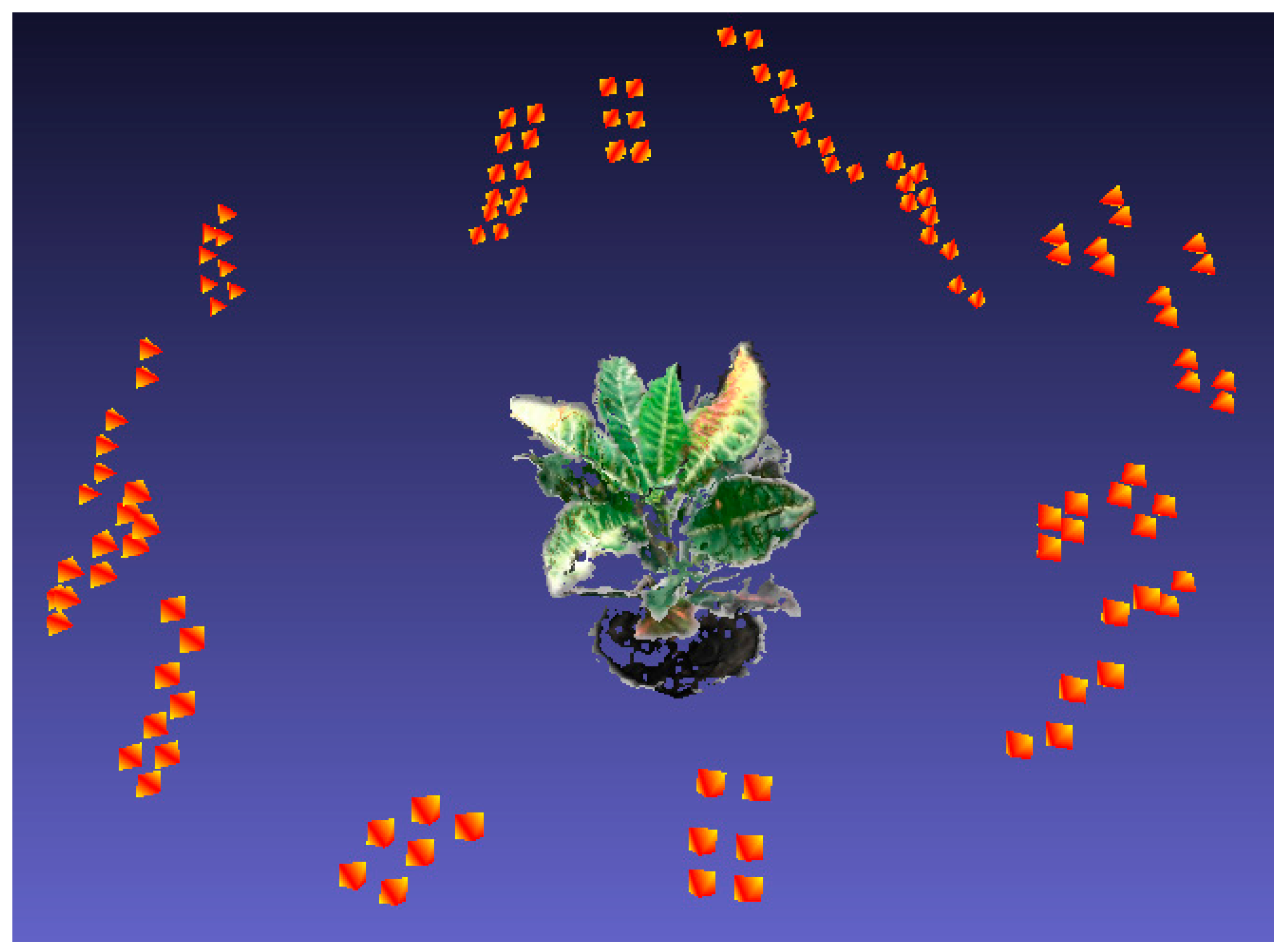
2.3. Image Acquisition

To make a full view reconstruction of the plant or tree, multiple images from different view angles had to be taken over the target. The stereo camera (shown in Figure 1) and a laptop with image acquisition software were used to acquire the images. One setup of the experiment is shown in Figure 5, where the target plant was in the center, and the stereo cameras positions are shown around it. The images taken from the adjacent locations should have an overlapping region.

2.4. Feature Points Detection and Matching

At the beginning, feature points were detected as Harris corners [41]. A pixel was selected as a salient pixel if its response was an eight-way local maximum. Normalized cross correlation (NCC) and normalized sum of squared differences (NSSD) described by Richard [42] could be used to match the features. Harris corner features were not invariant to affine and scale transform. Mikolajczyk and Schmid [43] provided different scale and affine invariant feature point detectors, such as Harris-Laplace and Harris-Affine. Mikolajczyk and Schmid [44] did a performance evaluation for four different local feature detectors (Harris-Laplace, Hessian-Laplace, Harris-Affine, and Hessian-Affine) and 10 different feature descriptors. Lowe [28] provided a Scale Invariant Feature Transform (SIFT) descriptor to describe the detected keypoints. Using Lowe’s SIFT research, Yan and Sukthankar [45] derived a PCA-based SIFT (PCA-SIFT), and Morel and Yu [46] provided an affine SIFT (ASIFT). To enhance the computing speed of SIFT, a speeded up robust features (SURF) was provided by Bay et al. [47]. To further improve the computation speed of SIFT, a parallel algorithm called SiftGPU was provided by Wu [35].
Snavely et al. [27] applied SIFT on multiple-view reconstruction from unordered images. Snavely [36] provided the software called Bundler to realize this method. In Snavely’s research, the SIFT feature points for each image were detected. Each pair of two images were then matched using ANN algorithm from Arya et al. [48]. This process was conducted in serial computation. The computation time required increased significantly as the number of input images and the number of feature points per image increased. Santos and Oliveira [34] applied Bundler on their plant phenotyping, and they reported that almost one hour would be needed to match the features for each two images of the total 143 images, and almost 30 min for 77 images.
Wu [37] provided a fast method called visual structure from motion (SfM) method to accelerate the feature points’ detection, matching, bundle adjustment, and 3D reconstruction. Wu’s method was applied in this paper.

2.5. Sparse Bundle Adjustment

Given a set of images, the matched feature points, also known as 2D projections, could be found through the feature matching algorithm introduced in the previous section. Each matched feature point had a corresponding 3D point in the scene. The camera matrices and 3D points could be estimated through bundle adjustment method [40]. The j-th 3D point X ^ j will be projected on the i-th image as x ^ j i through the i-th camera calibration matrix P ^ i , where x ^ j i = P ^ i X ^ j [40]. By minimizing the errors between re-projected projection x ^ j i and the actual projection x j i , the camera calibration matrix P ^ i , and sparse 3D points X ^ j could be estimated. A software package called sparse bundle adjustment (SBA) was provided by Lourakis and Argyros [49] to realize this minimization.

2.6. Dense 3D Reconstruction Using CMVS and PMVS

The patch model developed by Furukawa and Ponce [33,50] to produce 3D dense reconstruction from multiple view stereo (MVS) was used in this research. Patch was reconstructed through three steps: feature matching, patch expansion, and patch filtering. Feature matching was used to generate an initial bundle of patches. Then the patches were made denser. The outliers were removed by filtering. Finally, the patches were used to build a polygonal mesh. Furukawa and Ponce [51] developed software called PMVS to implement this method. PMVS used the output (camera matrices) from Bundler as the input. Other inputs for PMVS were from another software called CMVS [52].

2.7. Stereo Reconstruction Using VisualSFM

VisualSFM, which was proposed by Wu [37], integrated three technologies together: feature points detection and matching [35], multicore bundle adjustment [53], and dense 3D reconstruction [33]. Multiple images from a full view of the plant/tree would be imported into this software. A fully reconstructed result would be generated through the previously mentioned three steps.

2.8. Metric Reconstruction

The result from bundle adjustment was not metric reconstruction, which means that the reconstructed result did not show the actual size of the target.
A direct reconstruction method using ground truth was provided by Hartley and Zisserman [40] to realize the metric reconstruction. Using pre-calibrated stereo cameras, the Euclidean ground truth of a set of 3D points X e u c i could be solved from the 2D correspondence x 1 i x 2 i , and the estimated 3D points X e s t i could be obtained from bundle adjustment. The estimated 3D points and the Euclidean 3D points were related through a homography transformation (H). Then we have X e u c i = H · X e s t i . The first two images from the stereo camera were used to solve the Euclidean ground truth from the 2D projection. From our stereo camera calibration we knew that this stereo camera pair had good accuracy only when the distance between camera and the target was less than 580 mm. Therefore, those 3D points whose Z coordinates were bigger than 580 mm would be filtered as outliers.
To minimize the homography fitting error, these two sets of 3D points had to be normalized. After normalization, using the method described by Hartley and Zisserman [40], the centroid of the new points was at the origin, and the average distance from the origin is 3 . After applying normalization, X n e w p t s 1 i =   T 1 · X e u c i and X n e w p t s 2 i =   T 2 · X e s t i the homography between { X n e w p t s 1 i } and { X n e w p t s 2 i } was estimated using rigid transformation Forsyth and Ponce [54]. By fitting rigid transformation, we get X n e w p t s 1 i = H e s t · X n e w p t s 2 i . To de-normalize it, we have X e u c i = H · X e s t i , where H = T 1 1 · H e s t · T 2 . Applying H on all the 3D points from bundle adjustment, we can transfer them back to metric scale. The new camera calibration matrix was P e u c i = P e s t i · H 1 .

3. Experimental Results and Discussion

Four test experiments were conducted, one was a box with known geometry, and the other three were a croton plant with salient features, a jalapeno pepper plant with medium-size leaves, and a lemon tree with small leaves.
Test 1: A hexagon box with a given geometry was used to verify the reconstruction result. The box was placed on the top of a table. The stereo camera was manually moved around the box to take the images. Images taken at the adjacent locations should have some overlap, which is good for feature matching. The side length of the hexagon is 64 mm, and the height is 70 mm. To give the box texture, paper with printed citrus leaf images was wrapped around the box, as shown in Figure 6. Approximately 86 images were taken from various positions around this box using the stereo camera. The box was first reconstructed by using VisualSFM [37]. The result is shown in Figure 7A. The box was then was reconstructed by applying the metric reconstruction method (mentioned in step 2.8). The result is shown in Figure 7B, which shows the real size of the target.
The reconstructed length for each side of the above hexagon and the reconstructed height of each side face are shown in Table 2 and Table 3.
From this verifying test, we can see that the hexagon box is well reconstructed. The estimated length and height of the box is very close to the actual size. This method was then applied to complicated objects, such as a plant and a small tree.
Test 2: Three kinds of plants with different leaf sizes were reconstructed using the method introduced. The croton plant has big and sparse leaves with salient features. The jalapeno pepper has medium and sparse leaves. The lemon tree has small and dense leaves. They are shown in Figure 8.
Firstly, the objects were reconstructed in projective views by using VisualSFM from Wu [37]. Then the metric reconstruction algorithm (mentioned in step 2.8) was applied to get the 3D reconstruction in Euclidean space. For croton plants, the first pair of images were used as the ground truth. The feature points for these two images were extracted and matched. Together with the camera matrices of the stereo cameras, the actual 3D points could be calculated by using triangulation method of Hartley and Zisserman [40]. The estimated 3D points for the same 2D correspondences could be found from the reconstructed results of VisulaSFM. By applying rigid transform, the transformation between actual 3D points and estimated 3D points could be achieved. Applying this transformation to all the estimated 3D points for all the images, the final metric 3D reconstruction could be obtained, which is shown in Figure 9A. A similar process was applied to the other two plants. For the pepper plant, the first pair of images was used, and for the lemon tree, the seventh pair of images was used. The reconstructed view of the target was displayed in a bounding box, which was shown in Figure 9B,C respectively.
To roughly calculate the volume of the reconstructed plant canopy, the bounding box was divided into voxels. If the 3D point is inside the voxel, then that voxel will be marked as used. Unused voxels will be removed, as shown in Figure 10. All the 3D reconstructed points reside inside some voxels. The summation of the volume of all these voxels will be the canopy volume. There is a tradeoff between the size of the voxel and the volume of canopy. This tradeoff was not analyzed in this research since it is not the primary task. The estimated volume for these three plants are shown in Table 4.

4. Conclusions

This paper demonstrated a new approach to calibrate the camera calibration matrix on a metric level and then implemented the VisualSFM method to make a projective reconstruction of a plant/tree canopy. Stereo cameras were employed to estimate the actual 3D points for image pairs. The projective reconstructed view was then transformed to metric reconstruction by applying rigid transformation. A verifying experiment was performed by reconstructing a hexagon box. The result showed that this method can reach the true size of the target object. The same method was applied on three kinds of plant/tree with different leaf sizes. The reconstructed results presented a good visual view in 3D with reconstructed leaf features retaining their defining characteristics. This approach provides a metric reconstruction method that can achieve real-size reconstruction, which is a significant accomplishment in practical applications such as, 3D visualization, plant phenotypeing, robotic harvesting, and precision spraying, where real-size characteristics of plants are important for successful production practices.

Acknowledgments

The authors would like to acknowledge the contribution to this research provided by sponsors GeoSpider, Inc. and their funding source through the USDA SBIR program. This research is supported in part by a grant from the United States Department of Agriculture Small Business Innovation Research (USDA-SBIR) award contract #2012-33610-19499 and the USDA NIFA AFRI National Robotics Initiative #2013-67021-21074.

Author Contributions

Zhijiang Ni was the principle researcher and author of the paper. Thomas F. Burks was the graduate advisor/mentor and conceiver of the project who oversaw research and writing and provided editorial support. Won Suk Lee was an advisor to the project and also provided editorial support.

Conflicts of Interest

The authors declare no conflict of interest.

References

  1. Sinoquet, H.; Moulia, B.; Bonhomme, R. Estimating the three-dimensional geometry of a maize crop as an input of radiation models: Comparison between three-dimensional digitizing and plant profiles. Agric. For. Meteorol. 1991, 55, 233–249. [Google Scholar] [CrossRef]
  2. Tumbo, S.D.; Salyani, M.; Whitney, J.D.; Wheaton, T.A.; Miller, W.M. Investigation of laser and ultrasonic ranging sensors for measurements of citrus canopy volume. Appl. Eng. Agric. 2002, 18, 367–372. [Google Scholar] [CrossRef]
  3. Zaman, Q.U.; Salyani, M. Effects of foliage density and ground speed on ultrasonic measurement of citrus tree volume. Appl. Eng. Agric. 2004, 20, 173–178. [Google Scholar] [CrossRef]
  4. Wei, J.; Salyani, M. Development of a laser scanner for measuring tree canopy characteristics: Phase 1. Prototype development. Trans. ASAE 2004, 47, 2101–2107. [Google Scholar] [CrossRef]
  5. Wei, J.; Salyani, M. Development of a laser scanner for measuring tree canopy characteristics: Phase 2. Foliage density measurement. Trans. ASAE 2005, 48, 1595–1601. [Google Scholar] [CrossRef]
  6. Lee, K.H.; Ehsani, R. A laser scanner based measurement system for quantification of citrus tree geometric characteristics. Appl. Eng. Agric. 2009, 25, 777–788. [Google Scholar] [CrossRef]
  7. Rosell, J.R.; Llorens, J.; Sanz, R.; Arnó, J.; Ribes-Dasi, M.; Masip, J.; Escolà, A.; Camp, F.; Solanelles, F.; Gràcia, F.; et al. Obtaining the three-dimensional structure of tree orchards from remote 2D terrestrial LIDAR scanning. Agric. For. Meteorol. 2009, 149, 1505–1515. [Google Scholar] [CrossRef]
  8. Sanz-Cortiella, R.; Llorens-Calveras, J.; Escola, A.; Arno-Satorra, J.; Ribes-Dasi, M.; Masip-Vilalta, J.; Camp, F.; Gracia-Aguila, F.; Solanelles-Batlle, F.; Planas-DeMarti, S.; et al. Innovative LIDAR 3D dynamic measurement system to estimate fruit-tree leaf area. Sensors 2011, 11, 5769–5791. [Google Scholar] [CrossRef] [PubMed]
  9. Zhu, C.; Zhang, X.; Hu, B.; Jaeger, M. Reconstruction of tree crown shape from scanned data. In Technologies for E-Learning and Digital Entertainment; Pan, Z., Zhang, X., Rhalibi, A., Woo, W., Li, Y., Eds.; Springer: Berlin, Germany, 2008; pp. 745–756. [Google Scholar]
  10. Cui, Y.; Schuon, S.; Chan, D.; Thrun, S.; Theobalt, C. 3D shape scanning with a time-of-flight camera. In Proceedings of the IEEE Conference on Computer Vision and Pattern Recognition, San Francisco, CA, USA, 13–18 June 2010; pp. 1173–1180.
  11. Shim, H.; Adelsberger, R.; Kim, J.; Rhee, S.M.; Rhee, T.; Sim, J.Y.; Gross, M.; Kim, C. Time-of-flight sensor and color camera calibration for multi-view acquisition. Vis. Comput. 2012, 28, 1139–1151. [Google Scholar] [CrossRef]
  12. Song, Y.; Glasbey, C.A.; Heijden, G.A.M.; Polder, G.; Dieleman, J.A. Combining stereo and time-of-flight images with application to automatic plant phenotyping. In Image Analysis; Heyden, A., Kahl, F., Eds.; Springer: Berlin, Germany, 2011; pp. 467–478. [Google Scholar]
  13. Boykov, Y.; Kolmogorov, V. An experimental comparison of min-cut/max- flow algorithms for energy minimization in vision. IEEE Trans. Pattern Anal. Mach. Intell. 2004, 26, 1124–1137. [Google Scholar] [CrossRef] [PubMed]
  14. Adhikari, B.; Karkee, M. 3D reconstruction of apple trees for mechanical pruning. In Proceedings of the ASABE Annual International Meeting, Louisville, KY, USA, 7–10 August 2011.
  15. Microsoft, Kinect for Xbox 360. Available online: http://www.xbox.com/en-US/KINECT (accessed on 10 March 2012).
  16. Izadi, S.; Kim, D.; Hilliges, O.; Molyneaux, D.; Newcombe, R.; Kohli, P.; Shotton, J.; Hodges, S.; Freeman, D.; Davison, A. KinectFusion: Real-time 3D reconstruction and interaction using a moving depth camera. In Proceedings of the 24th Annual ACM Symposium on User Interface Software and Technology, Santa Barbara, CA, USA, 16–19 October 2011; pp. 559–568.
  17. Newcombe, R.A.; Davison, A.J.; Izadi, S.; Kohli, P.; Hilliges, O.; Shotton, J.; Molyneaux, D.; Hodges, S.; Kim, D.; Fitzgibbon, A. KinectFusion: Real-time dense surface mapping and tracking. In Proceedings of the 10th IEEE International Symposium on Mixed and Augmented reality (ISMAR), Basel, Switzerland, 26–29 October 2011; pp. 127–136.
  18. Chene, Y.; Rousseau, D.; Lucidarme, P.; Bertheloot, J.; Caffier, V.; Morel, P.; Belin, E.; Chapeau-Blondeau, F. On the use of depth camera for 3D phenotyping of entire plants. Comput. Electron. Agric. 2012, 82, 122–127. [Google Scholar] [CrossRef] [Green Version]
  19. Azzari, G.; Goulden, M.; Rusu, R. Rapid characterization of vegetation structure with a Microsoft Kinect sensor. Sensors 2013, 13, 2384–2398. [Google Scholar] [CrossRef] [PubMed]
  20. Wang, Q.; Zhang, Q. Three-dimensional reconstruction of a dormant tree using RGB-D cameras. In Proceedings of the Annual International Meeting, Kansas City, MI, USA, 21–24 July 2013; p. 1.
  21. Zhang, W.; Wang, H.; Zhou, G.; Yan, G. Corn 3D reconstruction with photogrammetry. Int. Arch. Photogramm. Remote Sens. Spat. Inf. Sci. 2008, 37, 967–970. [Google Scholar]
  22. Song, Y. Modelling and Analysis of Plant Image Data for Crop Growth Monitoring in Horticulture. Ph.D. Thesis, University of Warwick, Coventry, UK, 2008. [Google Scholar]
  23. Han, S.; Burks, T.F. 3D reconstruction of a citrus canopy. In Proceedings of the 2009 ASABE Annual International Meeting, Reno, NV, USA, 21–24 June 2009.
  24. Pollefeys, M.; Koch, R.; van Gool, L. Self-calibration and metric reconstruction in spite of varying and unknown internal camera parameters. In Proceedings of the 6th International Conference on Computer Vision, Bombay, India, 4–7 January 1998; pp. 90–95.
  25. Pollefeys, M.; Koch, R.; Vergauwen, M.; van Gool, L. Automated reconstruction of 3D scenes from sequences of images. ISPRS J. Photogramm. Remote Sens. 2000, 55, 251–267. [Google Scholar] [CrossRef]
  26. Fitzgibbon, A.W.; Zisserman, A. Automatic camera recovery for closed or open image sequences. In Proceedings of the 5th European Conference on Computer Vision-Volume I, Freiburg, Germany, 2–6 June 1998; pp. 311–326.
  27. Snavely, N.; Seitz, S.M.; Szeliski, R. Photo tourism: Exploring photo collections in 3D. ACM Trans. Graph. 2006, 25, 835–846. [Google Scholar] [CrossRef]
  28. Lowe, D.G. Distinctive image features from scale-invariant keypoints. Int. J. Comput. Vis. 2004, 60, 91–110. [Google Scholar] [CrossRef]
  29. Quan, L.; Tan, P.; Zeng, G.; Yuan, L.; Wang, J.; Kang, S.B. Image-based plant modeling. ACM Trans. Graph. 2006, 25, 599–604. [Google Scholar] [CrossRef]
  30. Lhuillier, M.; Quan, L. A quasi-dense approach to surface reconstruction from uncalibrated images. IEEE Trans. Pattern Anal. Mach. Intell. 2005, 27, 418–433. [Google Scholar] [CrossRef] [PubMed]
  31. Tan, P.; Zeng, G.; Wang, J.; Kang, S.B.; Quan, L. Image-based tree modeling. ACM Trans. Graph. 2007, 26, 87. [Google Scholar] [CrossRef]
  32. Teng, C.H.; Kuo, Y.T.; Chen, Y.S. Leaf segmentation, classification, and three-dimensional recovery from a few images with close viewpoints. Opt. Eng. 2011, 50, 037003. [Google Scholar]
  33. Furukawa, Y.; Ponce, J. Accurate, dense, and robust multiview stereopsis. IEEE Trans. Pattern Anal. Mach. Intell. 2010, 32, 1362–1376. [Google Scholar] [CrossRef] [PubMed]
  34. Santos, T.T.; Oliveira, A.A. Image-based 3D digitizing for plant architecture analysis and phenotyping. In Proceedings of the Workshop on Industry Applications (WGARI) in SIBGRAPI 2012 (XXV Conference on Graphics, Patterns and Images), Ouro Preto, Brazil, 22–25 August 2012.
  35. Wu, C. SiftGPU: A GPU Implementation of Scale Invariant Feature Transform (SIFT). 2007. Available online: http://www.cs.unc.edu/~ccwu/siftgpu/ (accessed on 20 April 2013).
  36. Snavely, N. Bundler: Structure from Motion (SfM) for Unordered Image Collections. 2010. Available online: http://phototour.cs.washington.edu/bundler/ (accessed on 8 August 2011).
  37. Wu, C. VisualSFM: A Visual Structure from Motion System. 2011. Available online: http://homes.cs.washington.edu/~ccwu/vsfm/ (accessed on 20 April 2013).
  38. Zhang, Z. A flexible new technique for camera calibration. IEEE Trans. Pattern Anal. Mach. Intell. 2000, 22, 1330–1334. [Google Scholar] [CrossRef]
  39. Bouguet, J.Y. Camera Calibration ToolBox for Matlab. 2008. Available online: http://www.vision.caltech.edu/bouguetj/calib_doc/ (accessed on 27 October 2011).
  40. Hartley, R.; Zisserman, A. Multiple View Geometry in Computer Vision; Cambridge University Press: Cambridge, UK, 2003. [Google Scholar]
  41. Harris, C.; Stephens, M. A combined corner and edge detector. In Proceedings of the 4th Alvey Vision Conference, Manchester, UK, 31 August–2 September 1988; pp. 147–151.
  42. Richard, S. Computer Vision: Algorithms and Applications; Springer: Berlin, Germany, 2011. [Google Scholar]
  43. Mikolajczyk, K.; Schmid, C. Scale & affine invariant interest point detectors. Int. J. Comput. Vis. 2004, 60, 63–86. [Google Scholar]
  44. Mikolajczyk, K.; Schmid, C. A performance evaluation of local descriptors. IEEE Trans. Pattern Anal. Mach. Intell. 2005, 27, 1615–1630. [Google Scholar] [CrossRef] [PubMed]
  45. Yan, K.; Sukthankar, R. PCA-SIFT: A more distinctive representation for local image descriptors. In Proceedings of the IEEE Computer Society Conference on Computer Vision and Pattern Recognition, Washington, DC, USA, 27 June–2 July 2004; Volume 502, pp. II-506–II-513.
  46. Morel, J.M.; Yu, G. ASIFT: A new framework for fully affine invariant image comparison. SIAM J. Imaging Sci. 2009, 2, 438–469. [Google Scholar] [CrossRef]
  47. Bay, H.; Tuytelaars, T.; van Gool, L. Surf: Speeded up robust features. In Proceedings of the 9th European Conference on Computer Vision, Graz, Austria, 7–13 May 2006.
  48. Arya, S.; Mount, D.M.; Netanyahu, N.S.; Silverman, R.; Wu, A.Y. An optimal algorithm for approximate nearest neighbor searching fixed dimensions. J. ACM 1998, 45, 891–923. [Google Scholar] [CrossRef]
  49. Lourakis, M.I.A.; Argyros, A.A. SBA: A software package for generic sparse bundle adjustment. ACM Trans. Math. Softw. 2009, 36, 1–30. [Google Scholar] [CrossRef]
  50. Furukawa, Y.; Ponce, J. Accurate, dense, and robust multi-view stereopsis. In Proceedings of the IEEE Conference on Computer Vision and Pattern Recognition, Minneapolis, MN, USA, 17–22 June 2007; pp. 1–8.
  51. Furukawa, Y.; Ponce, J. Patch-Based Multi-View Stereo Software (PMVS—Version 2). 2010. Available online: http://www.di.ens.fr/pmvs/ (accessed on 9 September 2012).
  52. Furukawa, Y. Clustering Views for Multi-View Stereo (CMVS). 2010. Available online: http://www.di.ens.fr/cmvs/ (accessed on 9 September 2012).
  53. Wu, C.C.; Agarwal, S.; Curless, B.; Seitz, S.M. Multicore bundle adjustment. In Proceedings of the IEEE Conference on Computer Vision and Pattern Recognition, Colorado Springs, CO, USA, 20–25 June 2011; pp. 3057–3064.
  54. Forsyth, D.A.; Ponce, J. Computer Vision: A Modern Approach; Prentice Hall: Upper Saddle River, NJ, USA, 2003. [Google Scholar]
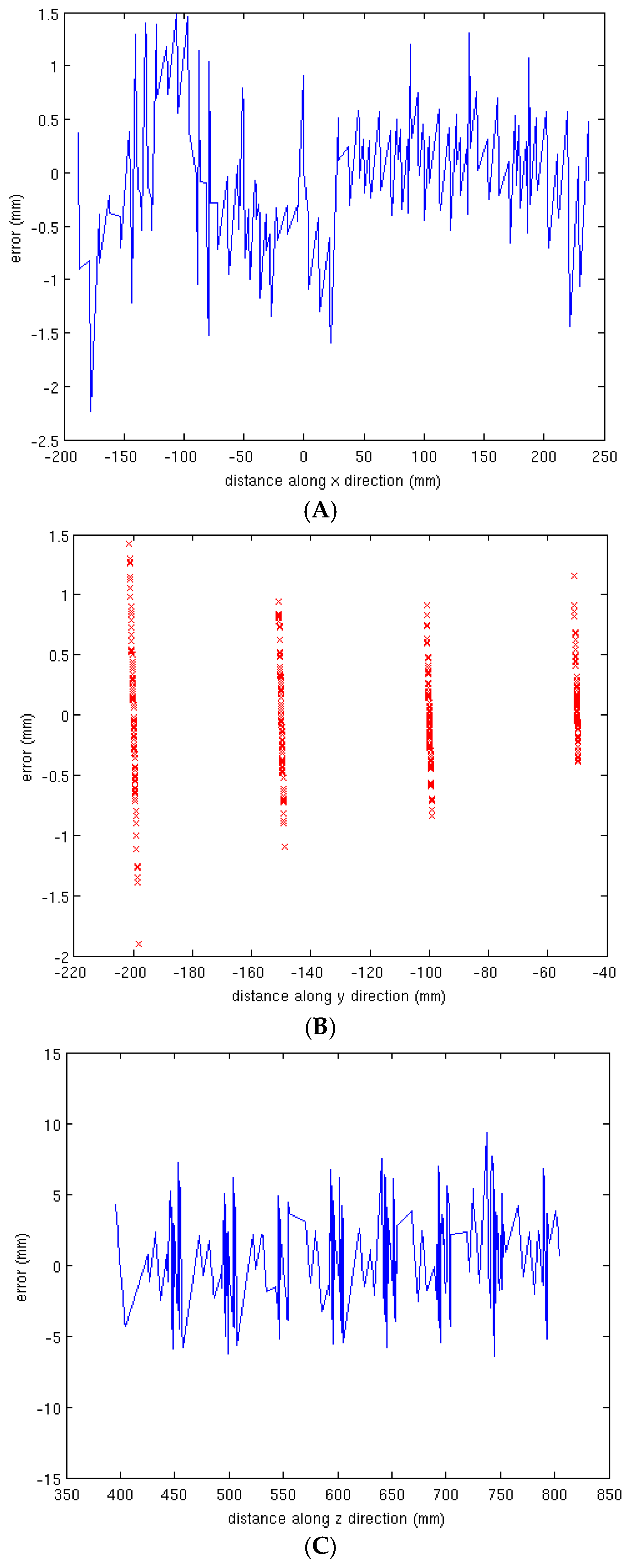
Figure 1. Stereo cameras which are used to acquire images: (A) whole view; (B) inside view.
Jimaging 02 00028 g001
Figure 2. World coordinate system (2D x-z system plus vertical checkerboard).
Jimaging 02 00028 g002
Figure 3. 2D x-z coordinate system (each line is 50 mm separated).
Jimaging 02 00028 g003
Figure 4. Error plots in X, Y, and Z direction. (A) errors in x direction; (B) errors in y direction; (C) errors in z direction.
Jimaging 02 00028 g004
Figure 5. An example of stereo camera setup for image acquisition with the 3D reconstruction results (56 stereo pairs were used).
Jimaging 02 00028 g005
Figure 6. Hexagon box with texture.
Jimaging 02 00028 g006
Figure 7. 3D reconstruction. (A) projective reconstruction; (B) metric reconstruction.
Jimaging 02 00028 g007
Figure 8. Experimental plants/tree: (A) Croton plant; (B) Jalapeno pepper plant; (C) Lemon tree.
Jimaging 02 00028 g008
Figure 9. Reconstructed plants. (A) croton; (B) pepper; (C) lemon.
Jimaging 02 00028 g009
Figure 10. Demo of volume calculation. (A) Bounding box was divided into voxels; (B) Voxels left after removing unused voxels.
Jimaging 02 00028 g010
Table 1. Statistical analysis of errors between estimated and actual corners.
AxisMean Absolute Error (mm)Standard Deviation (mm)
X0.420.35
Y0.360.31
Z2.781.74
Table 2. Estimated length vs. actual length.
LengthL1L2L3L4L5L6
Estimated length (mm)64.1963.4768.8265.5963.0061.99
Actual length (mm)64.0064.0064.0064.0064.0064.00
error (mm)0.19−0.534.821.59−1.00−2.01
Table 3. Estimated height vs. actual height.
HeightH1H2H3H4H5H6
Estimated height (mm)70.4568.5371.1068.1370.6869.03
Actual height (mm)70.0070.0070.0070.0070.0070.00
error (mm)0.45−1.471.10−1.830.68−0.97
Table 4. Volumes of these three plants.
Experimental Targets# of Voxel Hits/# of Total 3D PointsVoxel Size (mm3)Volume (cm3)
Croton16,156/19,57928.461.23 × 103
Jalapeno pepper28,591/38,77312.613.61 × 102
Lemon tree48,609/96,6803.761.83 × 102

