
Active Infrared Thermography for Seal Contamination Detection in Heat-Sealed Food Packaging


Abstract
:
1. Introduction
2. Related Work
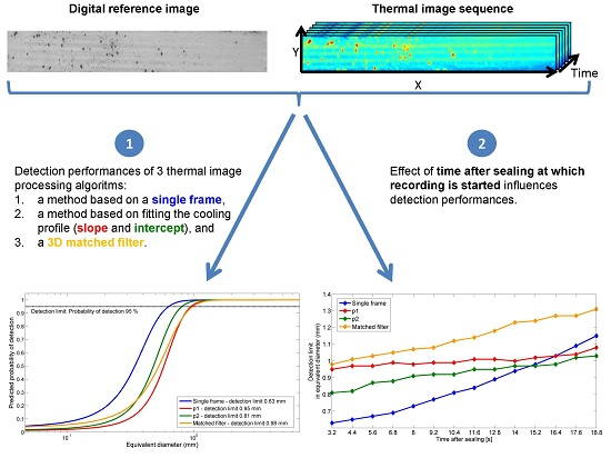
3. Objective
4. Materials and Methods
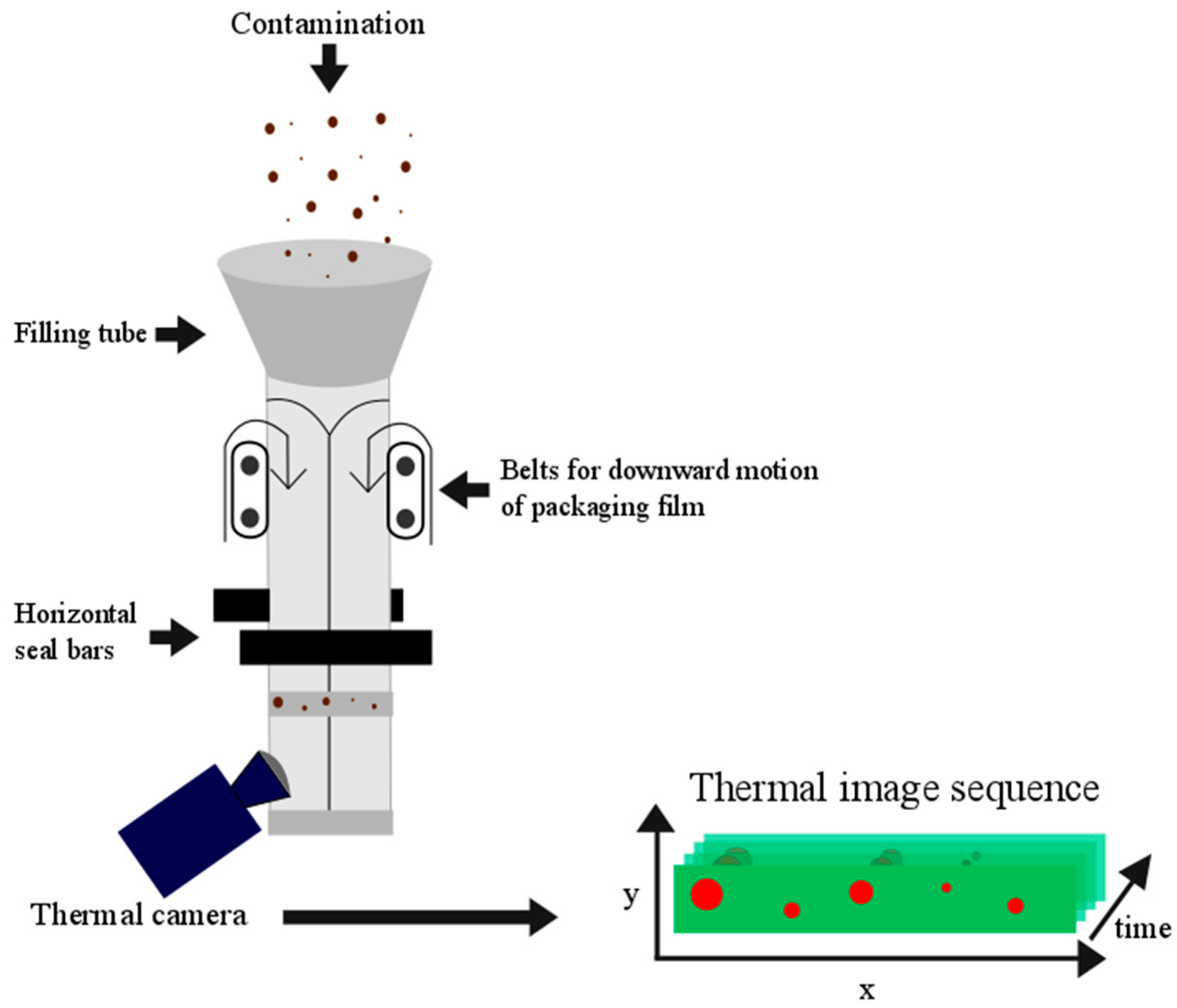
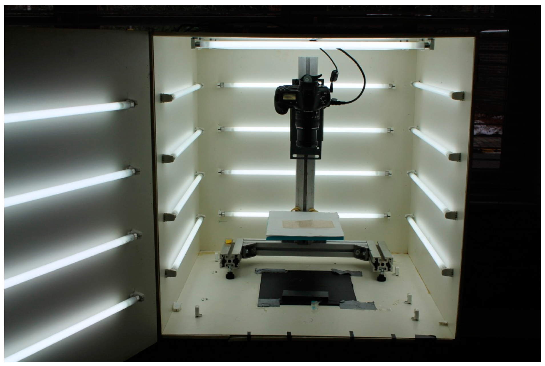
4.1. Sample Preparation and Image Acquisition
4.2. Preprocessing of the Thermal Image Sequences
4.3. Processing of the Thermal Image Sequences
4.3.1. Single Frame
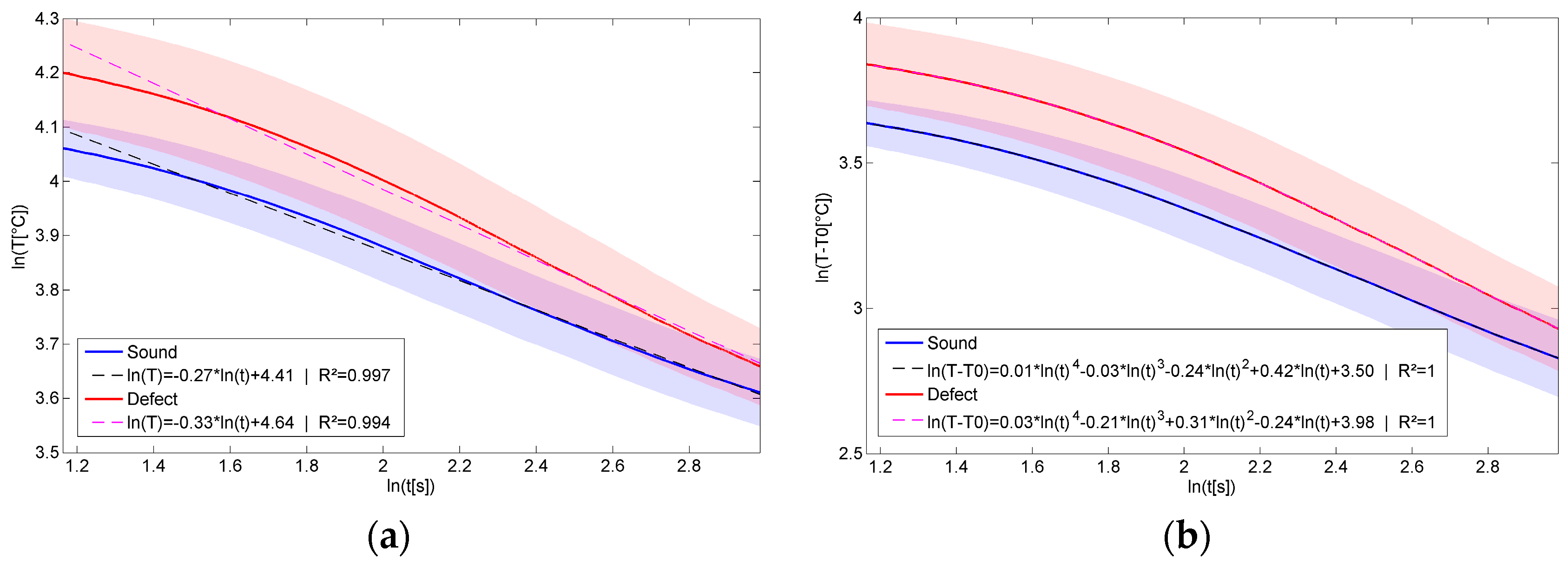
4.3.2. Fit of the Cooling Profiles
4.3.3. Thermal Signal Reconstruction
4.3.4. Pulsed Phase Thermography
4.3.5. Principal Component Thermography
4.3.6. Matched Filter
4.4. Comparison of Image Processing Methods
4.4.1. Image Registration
4.4.2. Image Binarization
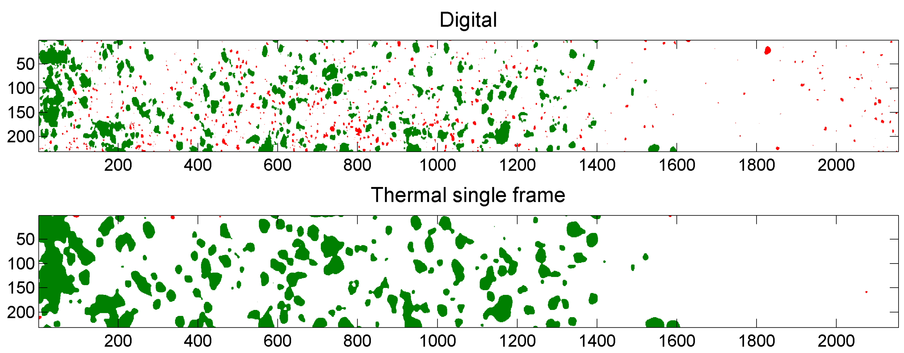
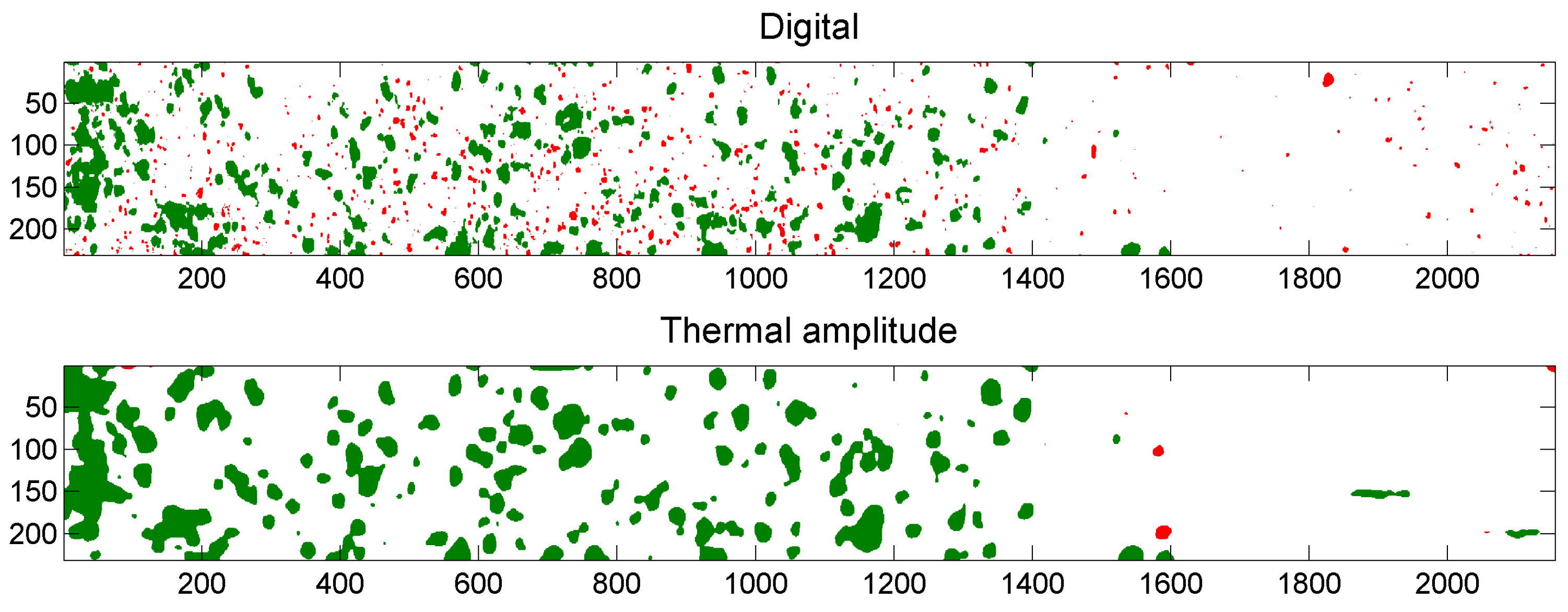
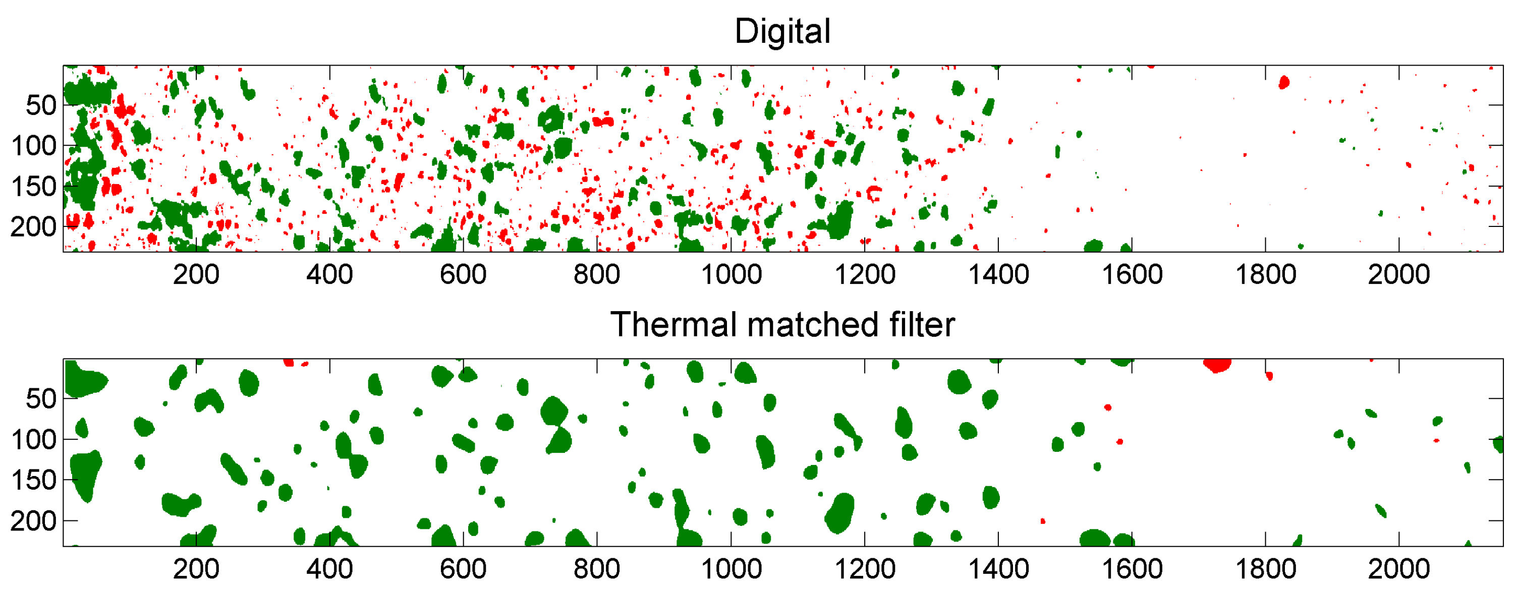
4.4.3. Comparison of Digital and Thermal Images
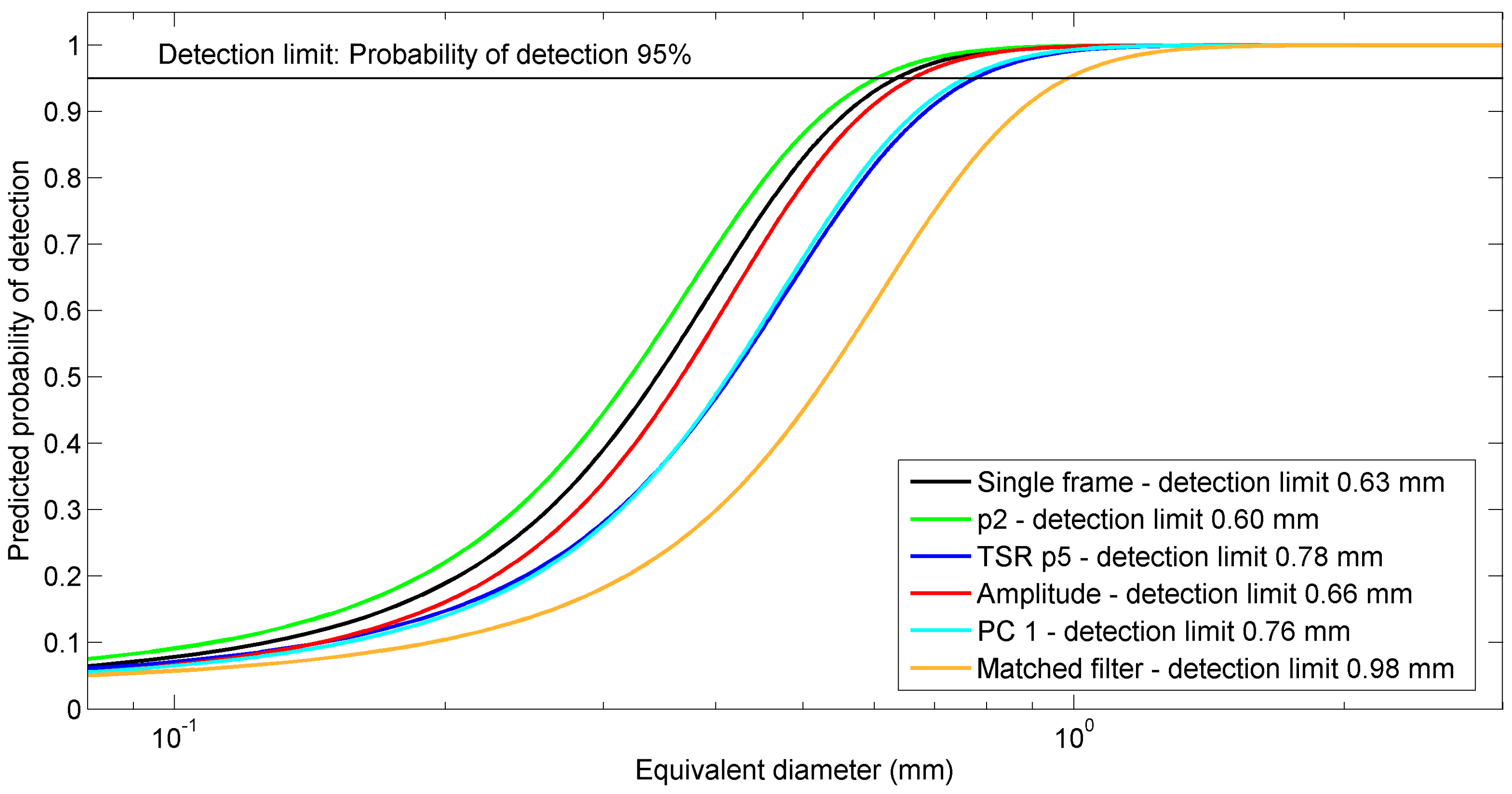
4.4.4. Calculation of Detection Limits
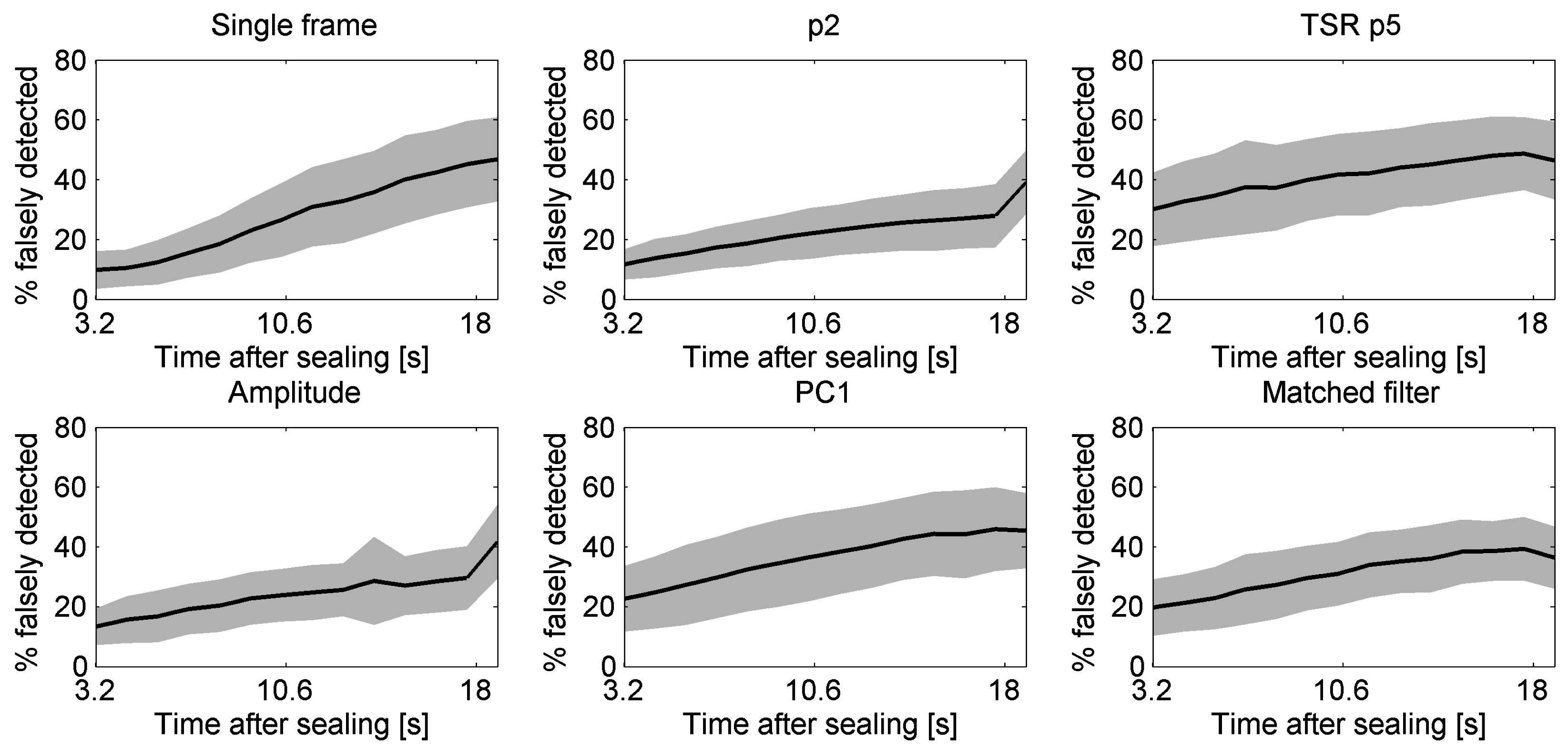
4.4.5. Effect of Start Time of Recording after Sealing on Detection Performances
5. Results
5.1. Example of First Order Fit and Thermal Signal Reconstruction of the Cooling Profiles
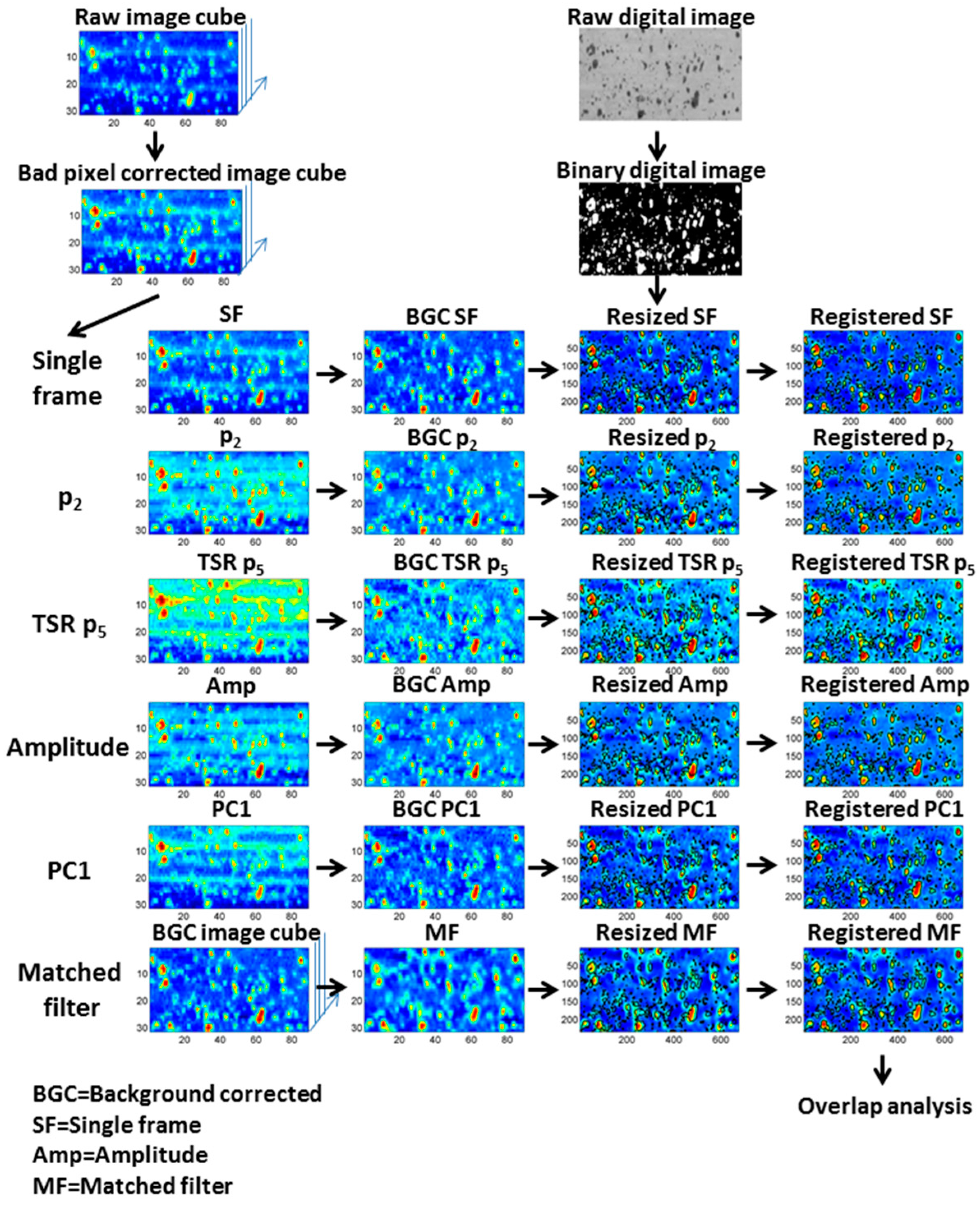
5.2. Overview of Image Processing Steps
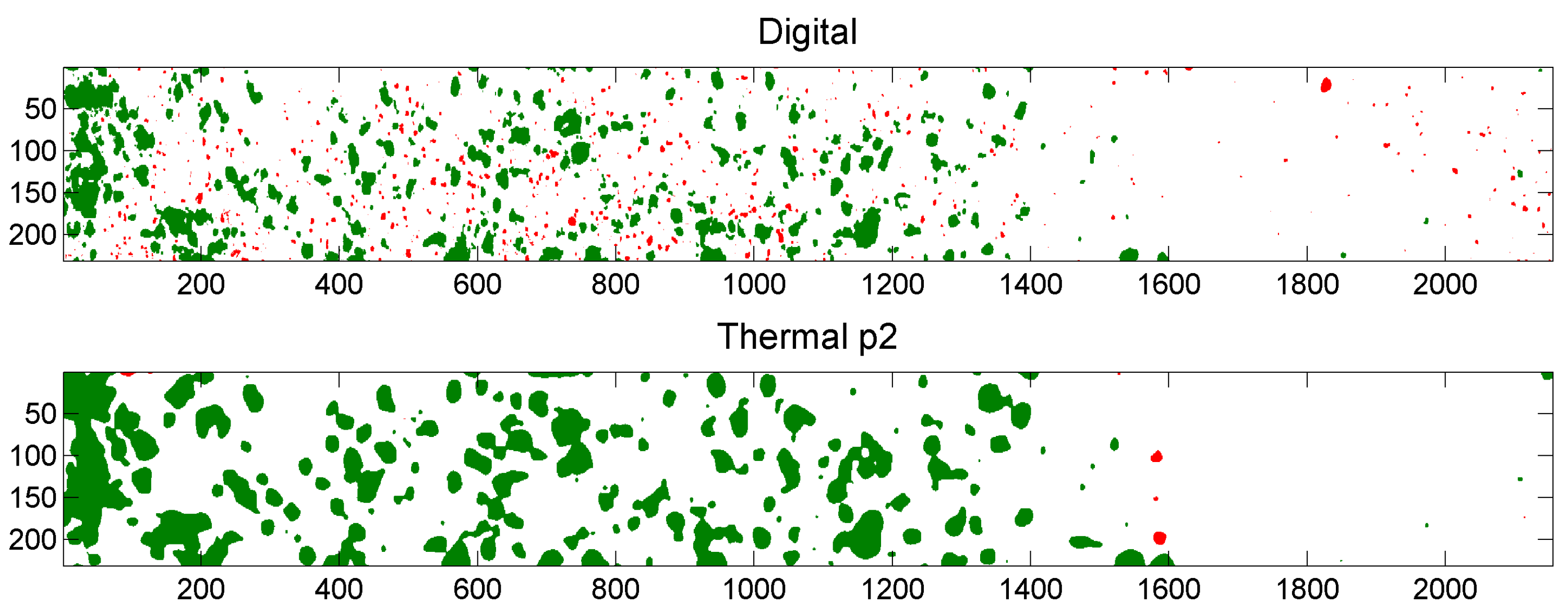
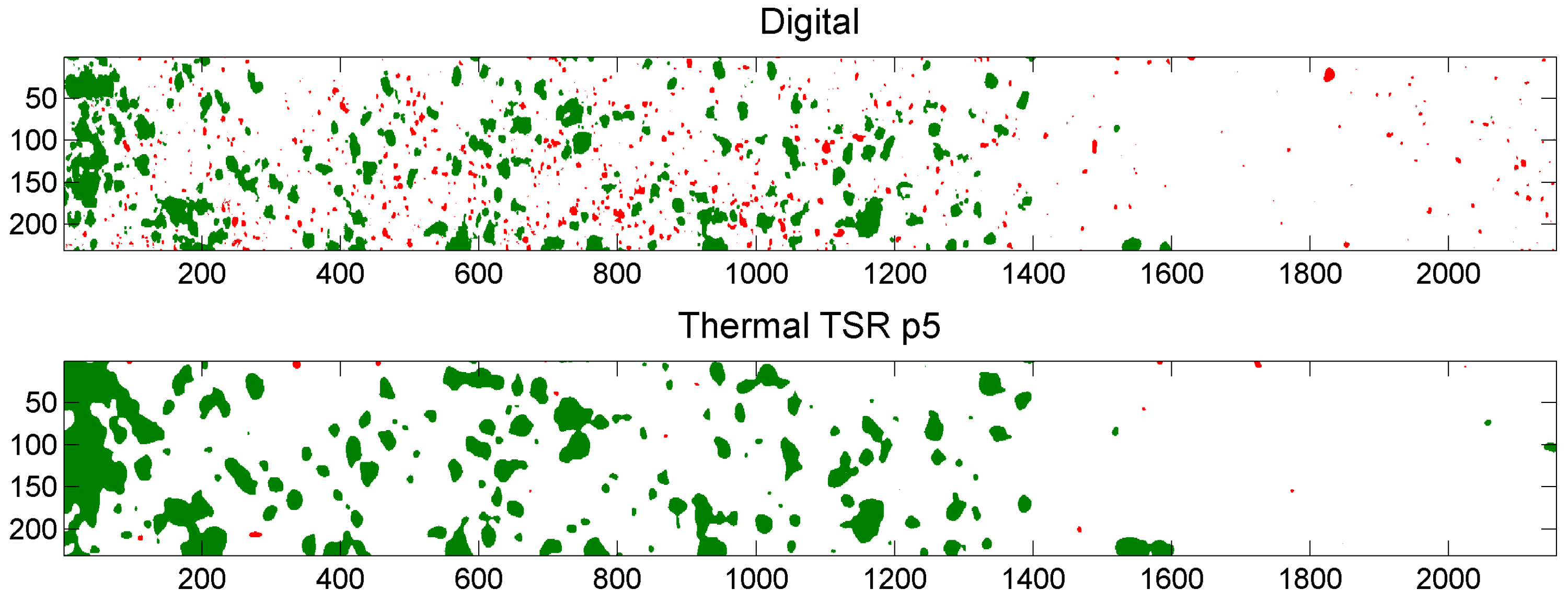
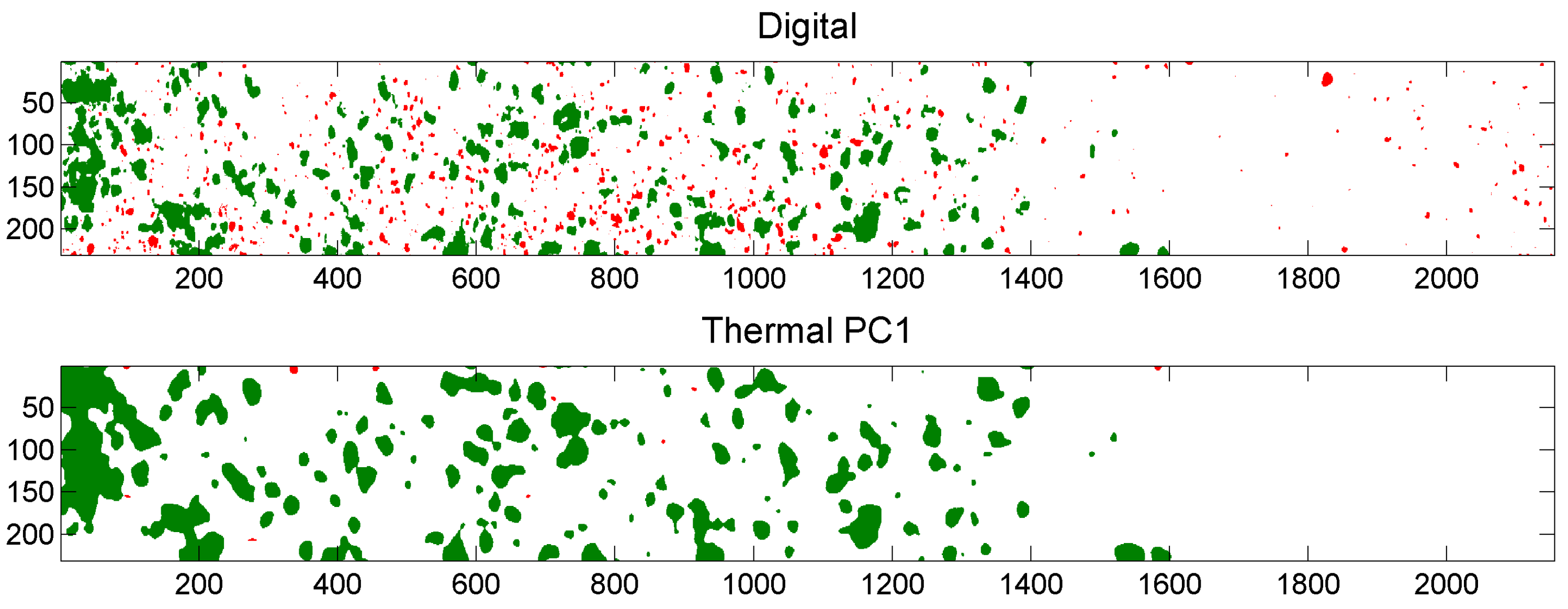
5.3. Example of Overlap Visualization
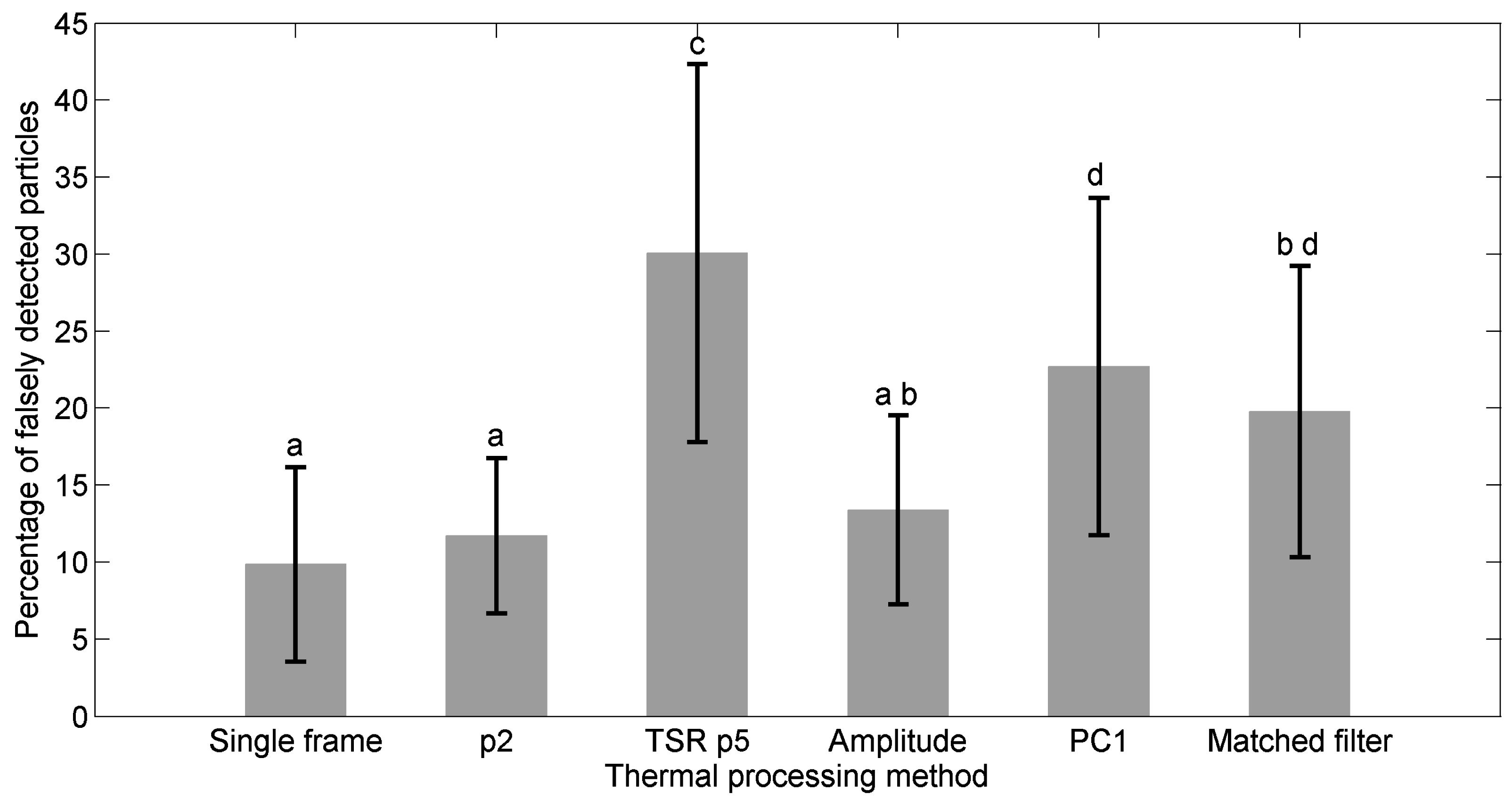
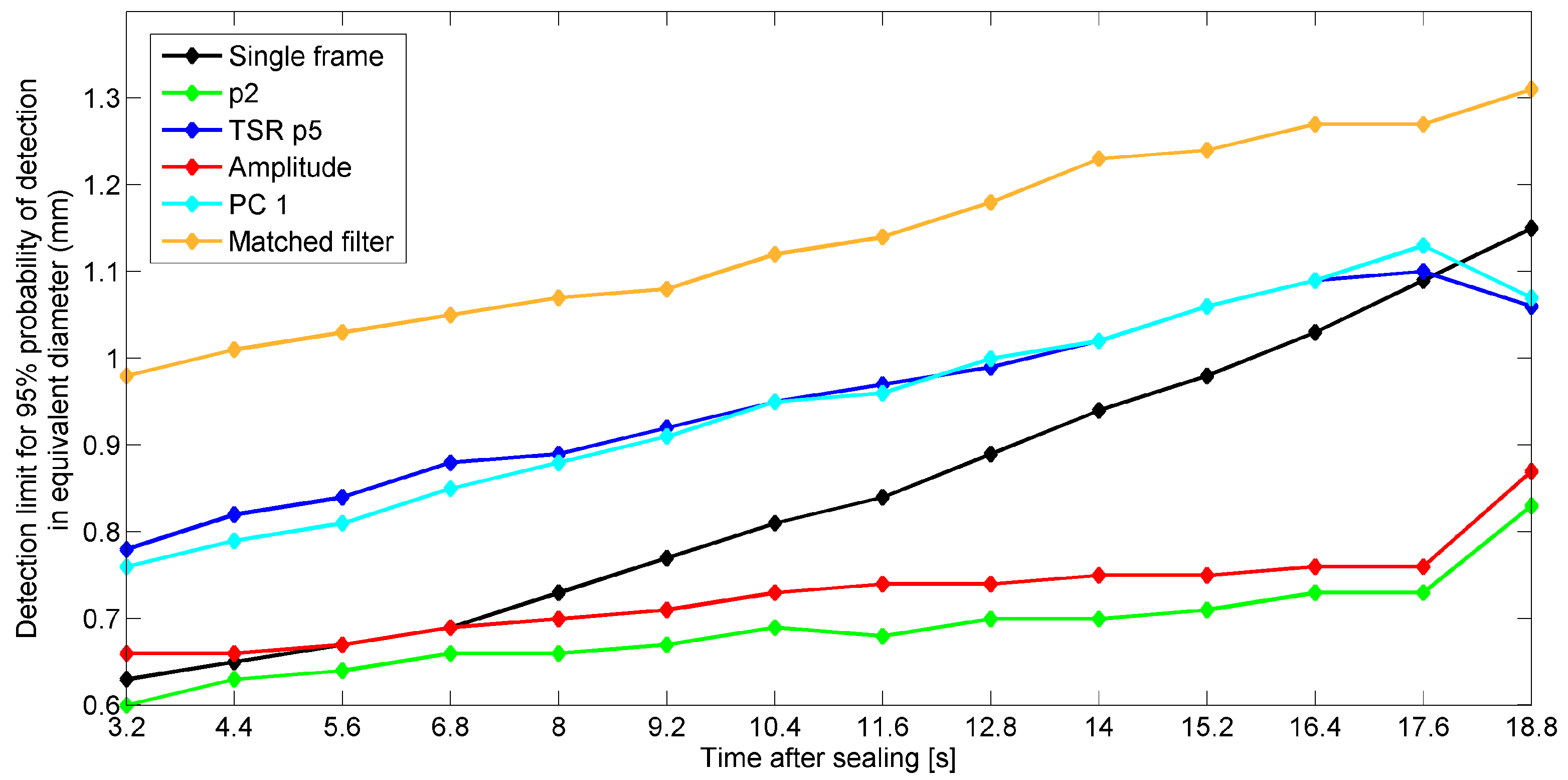
5.4. Comparison of Detection Performances of the Thermal Data Processing Methods
5.5. Effect of Start Time of Recording after Sealing on Detection Performances
6. Discussion
7. Conclusions
Acknowledgments
Author Contributions
Conflicts of Interest
References
- Robertson, G.L. Food Packaging: Principles and Practice; CRC Press Taylor & Francis Group: Boca Raton, FL, USA, 2013. [Google Scholar]
- Dudbridge, M. Handbook of Seal Integrity in the Food Industry, 1st ed.; John Wiley & Sons: West Sussex, UK, 2016. [Google Scholar]
- Ostyn, B.; Darius, P.; De Baerdemaeker, J.; De Ketelaere, B. Statistical monitoring of a sealing process by means of multivariate accelerometer data. Qual. Eng. 2007, 19, 299–310. [Google Scholar] [CrossRef]
- Ozguler, A.; Morris, S.A.; O’Brien, W.D., Jr. Ultrasonic imaging of micro-leaks and seal contamination in flexible food packages by the pulse-echo technique. J. Food Sci. 1998, 63, 673–678. [Google Scholar] [CrossRef]
- Lampi, R.A.; Schulz, G.L.; Ciavarini, T.; Burke, P.T. Performance and integrity of retort pouch seals. Food Technol. 1976, 30, 38–48. [Google Scholar]
- Frazier, C.H.; Tian, Q.; Ozguler, A.; Morris, S.A.; O’Brien, W.D., Jr. High contrast ultrasound images of defects in food package seals. IEEE Trans. Ultrason. Ferroelectr. Freq. Control 2000, 47, 530–539. [Google Scholar] [CrossRef] [PubMed]
- Mihindukulasuriya, S.; Lim, L.-T. Effects of liquid contaminants on heat seal strength of low-density polyethylene film. Packag. Technol. Sci. 2011, 25, 271–284. [Google Scholar] [CrossRef]
- Bach, S.; Thürling, K.; Majschak, J.-P. Ultrasonic sealing of flexible packaging films—Principles and characteristics of an alternative sealing method. Packag. Technol. Sci. 2012, 25, 233–248. [Google Scholar] [CrossRef]
- Pascall, M.A.; Richtsmeier, J.; Riemer, J.; Farahbakhsh, B. Non-destructive packaging seal strength analysis and leak detection using ultrasonic imaging. Packag. Technol. Sci. 2002, 15, 275–285. [Google Scholar] [CrossRef]
- ASTM F2338. Standard Test Method for Nondestructive Detection of Leaks in Packages by Vacuum Decay Method; Active Standard ASTM: West Conshohocken, PA, USA, 2013. [Google Scholar]
- ASTM F2391-05. Standard Test Method for Measuring Package and Seal Integrity Using Helium as the Tracer Gas; Active Standard ASTM: West Conshohocken, PA, USA, 2011. [Google Scholar]
- Morita, Y.; Dobroiu, A.; Otani, C.; Kawase, K. Real-time terahertz diagnostics for detecting microleak defects in the seals of flexible plastic packaging. J. Adv. Mech. Des. Syst. 2007, 1, 338–345. [Google Scholar] [CrossRef]
- Shuangyang, Z. Fast inspection of food packing seals using machine vision. In Proceedings of the International Conference on Digital Manufacturing & Automation, Changcha, China, 18–20 December 2010; pp. 724–726.
- Barnes, M.; Dudbridge, M.; Duckett, T. Polarised light stress analysis and laser scatter imaging for non-contact inspection of heat seals in food trays. J. Food Eng. 2012, 112, 183–190. [Google Scholar] [CrossRef] [Green Version]
- Song, Y.S.; Gera, M.; Jain, B.; Koontz, J.L. Evaluation of a non-destructive high-voltage technique for the detection of pinhole leaks in flexible and semi-rigid packages for foods. Packag. Technol. Sci. 2014, 27, 423–436. [Google Scholar] [CrossRef]
- Maldague, X.P.V. Theory and Practice of Infrared Technology for Nondestructive Testing; Wiley: New York, NY, USA, 2001. [Google Scholar]
- Ibarra-Castanedo, C.; Tarpani, J.R.; Maldague, X.P.V. Nondestructive testing with thermography. Eur. J. Phys. 2013, 34, S91–S109. [Google Scholar] [CrossRef]
- Ignatowicz, S. Method and Apparatus for Analyzing Thermo-Graphic images to Detect Defects in Thermally Sealed Packaging. U.S. Patent 2007/0237201 A1, 11 October 2007. [Google Scholar]
- Ibarra-Castanedo, C.; González, D.; Klein, M.; Pilla, M.; Vallerand, S.; Maldague, X. Infrared image processing and data analysis. Infrared Phys. Technol. 2004, 46, 75–83. [Google Scholar] [CrossRef]
- Shepard, S.M. Temporal Noise Reduction, Compression and Analysis of Thermographic Image Data Sequences. U.S. Patent 6,516,084, 4 February 2003. [Google Scholar]
- Shepard, S.M.; Lhota, J.R.; Rubadeux, B.A.; Wang, D.; Ahmed, T. Reconstruction and enhancement of active thermographic image sequences. Opt. Eng. 2003, 42, 1337–1342. [Google Scholar] [CrossRef]
- Li, M.; Holland, S.D.; Meeker, W.Q. Statistical methods for automatic crack detection based on vibrothermography sequence-of-images data. Appl. Stoch. Models Bus. 2010, 26, 481–495. [Google Scholar] [CrossRef]
- Yoo, J.C.; Han, T.H. Fast normalized cross-correlation. Circ. Syst. Signal Process. 2009, 28, 819–843. [Google Scholar] [CrossRef]
- D’huys, K.; Saeys, W.; De Ketelaere, B. Detection of seal contamination in heat sealed food packaging based on active infrared thermography. In Proceedings of the Thermosense: Thermal Infrared Applications XXXVII, Baltimore, MD, USA, 20–24 April 2015.
- Ibarra-Castanedo, C.; Piau, J.-M.; Guilbert, S.; Avdelidis, N.P.; Genest, M.; Bendada, A.; Maldague, X.P.V. Comparative study of active thermography techniques for the nondestructive evaluation of honeycomb structures. Res. Nondestruct. Eval. 2009, 20, 1–31. [Google Scholar] [CrossRef]
- Rajic, N. Principal component thermography for flaw contrast enhancement and flaw depth characterization in composite structures. Compos. Struct. 2002, 58, 521–528. [Google Scholar] [CrossRef]
- Lewis, J.P. Fast normalized cross-correlation. Vis. Interface 1995, 10, 120–123. [Google Scholar]
- Brunelli, R. Template Matching Techniques in Computer Vision Theory and Practice; Wiley: New York, NY, USA, 2009. [Google Scholar]
- Briechle, K.; Hanebeck, U.D. Template matching using fast normalized cross correlation. In Proceedings of the Optical Pattern Recognition XII, Orlando, FL, USA, 16 April 2001.
- Otsu, N. A threshold selection method from gray-level histograms. IEEE Trans. Syst. Man Cybern. 1979, 9, 62–66. [Google Scholar] [CrossRef]
- Zack, G.W.; Rogers, W.E.; Latt, S.A. Automatic measurement of sister chromatid exchange frequency. J. Histochem. Cytochem. 1977, 25, 741–753. [Google Scholar] [CrossRef] [PubMed]
- Hochberg, Y.; Tamhane, A.C. Multiple Comparison Procedures; John Wiley & Sons: Hoboken, NJ, USA, 1987. [Google Scholar]
- Agresti, A. Categorical Data Analysis; Wiley: New York, NY, USA, 2012. [Google Scholar]


| Predictor | Estimate | Standard Error | p-Value |
|---|---|---|---|
| Intercept | −3.475 | 0.016 | <0.0001 |
| X1 | 0.419 | 0.016 | <0.0001 |
| X2 | −0.073 | 0.017 | <0.0001 |
| X3 | 0.028 | 0.017 | 0.1129 |
| X4 | −0.132 | 0.018 | <0.0001 |
| X5 | −0.465 | 0.019 | <0.0001 |
| D | 8.960 | 0.059 | <0.0001 |
| X1 × D | 1.477 | 0.141 | <0.0001 |
| X2 × D | −0.793 | 0.126 | 0.0001 |
| X3 × D | 1.000 | 0.139 | <0.0001 |
| X4 × D | −0.408 | 0.129 | 0.0016 |
| X5 × D | −2.457 | 0.115 | <0.0001 |
| Method | Processing Time per Sample |
|---|---|
| Single frame | 0.42 s |
| p2 (1st order fit) | 8.63 s |
| TSR p5 (4th order fit) | 19.06 s |
| Amplitude (PPT) | 3.93 s |
| PC1 (PCT) | 3.40 s |
| Matched filter | 24.76 s |
© 2016 by the authors; licensee MDPI, Basel, Switzerland. This article is an open access article distributed under the terms and conditions of the Creative Commons Attribution (CC-BY) license (http://creativecommons.org/licenses/by/4.0/).
Share and Cite
D’huys, K.; Saeys, W.; De Ketelaere, B. Active Infrared Thermography for Seal Contamination Detection in Heat-Sealed Food Packaging. J. Imaging 2016, 2, 33. https://doi.org/10.3390/jimaging2040033
D’huys K, Saeys W, De Ketelaere B. Active Infrared Thermography for Seal Contamination Detection in Heat-Sealed Food Packaging. Journal of Imaging. 2016; 2(4):33. https://doi.org/10.3390/jimaging2040033
Chicago/Turabian StyleD’huys, Karlien, Wouter Saeys, and Bart De Ketelaere. 2016. "Active Infrared Thermography for Seal Contamination Detection in Heat-Sealed Food Packaging" Journal of Imaging 2, no. 4: 33. https://doi.org/10.3390/jimaging2040033