Article

3D Imaging with a Sonar Sensor and an Automated 3-Axes Frame for Selective Spraying in Controlled Conditions

by
David Reiser
*,
Javier M. Martín-López
,
Emir Memic
,
Manuel Vázquez-Arellano
,
Steffen Brandner
and
Hans W. Griepentrog
Institute of Agricultural Engineering, University of Hohenheim, Garbenstraße 9, 70599 Stuttgart, Germany
*
Author to whom correspondence should be addressed.
J. Imaging 2017, 3(1), 9; https://doi.org/10.3390/jimaging3010009
Submission received: 30 December 2016 / Revised: 3 February 2017 / Accepted: 4 February 2017 / Published: 8 February 2017

Abstract

:
Autonomous selective spraying could be a way for agriculture to reduce production costs, save resources, protect the environment and help to fulfill specific pesticide regulations. The objective of this paper was to investigate the use of a low-cost sonar sensor for autonomous selective spraying of single plants. For this, a belt driven autonomous robot was used with an attached 3-axes frame with three degrees of freedom. In the tool center point (TCP) of the 3-axes frame, a sonar sensor and a spray valve were attached to create a point cloud representation of the surface, detect plants in the area and perform selective spraying. The autonomous robot was tested on replicates of artificial crop plants. The location of each plant was identified out of the acquired point cloud with the help of Euclidian clustering. The gained plant positions were spatially transformed from the coordinates of the sonar sensor to the valve location to determine the exact irrigation points. The results showed that the robot was able to automatically detect the position of each plant with an accuracy of 2.7 cm and could spray on these selected points. This selective spraying reduced the used liquid by 72%, when comparing it to a conventional spraying method in the same conditions.

1. Introduction

Pesticides are one of the main contamination factors of water sources and ecosystems in the world [1]. In the European Union, for example, a rate of 300,000 tons of pesticides were applied each year. This led to a water pollution that exceeded the threshold set by the regulation commission of the European Union (No. 546/2011) [2]. However, the excess of weeds increases the cost of the cultural practices, destroys crops, modifies the effectiveness of agricultural equipment and decreases the fertility of soils [3,4]. This leads to the assumption that the productivity of conventional farming is dependent on chemicals [3]. Although the use of pesticides, fungicides and fertilizers contributes to improving the quality and productivity of crops in agriculture, significant problems were reported when the chemicals are applied uniformly over the fields. Typical related problems are the negative effects on the environment [1,5], herbicide-resistant weeds [6] and human and animal health issues [7]. A decrease of the distributed chemicals, would not only result in a decrease in the contamination of ecosystems [8], but also in a reduction of costs and an increase of crop production efficiency [9]. Therefore, one goal for future farming should be to apply chemicals just at the place where they are required [10]. Instead of applying fixed amounts of pesticides over the field, each plant could be detected individually and treated when needed [11]. Modern technology should already be able to reduce the amount of the application, working time and environmental damage [11,12]. However, this requires robust and reliable sensors, software processing and application systems [13,14].
The technologies for the automatic detection and removal of weeds progressed significantly in the last decades. This was mainly because of the use of new sensor types and improvements in crop management and control treatments with herbicides, pesticides or fungicides [10,11,15,16]. Many investigations have focused on the use of image analysis techniques, stereo photogrammetry, spectral cameras, time-of-flight-cameras, structured light sensors and light detection and ranging (LiDAR) laser sensors [4,17,18,19,20]. Typically, the sensors were used on tractor implements to recognize the weeds and to use this information for selective spraying [21], or on robots, to automate the whole navigation and application process of selective spraying [12].
However, most of the mentioned sensor principles are limited by the high costs and/or complexity to acquire and to process the information [22]. This brings difficulty for the farmer to implement this technology, as agricultural machinery should have a good cost-benefit rate.
Since the new Microsoft Kinect v2 sensor (Microsoft, Redmond, WA, USA) was introduced to the consumer market, it was also used in agricultural research for environment perception [23,24,25,26]. This time-of-flight based sensor system is quite promising but is still highly affected by sunlight and requires high computational resources to process the data [23].
Using sonar sensors for selective spraying was already part of several research papers. Research was conducted comparing LiDAR systems with ultrasonic sensors to estimate the vegetation. The results indicated a good correlation between the estimation made by LiDAR and ultrasonic sensors [27]. The first sprayer with automatic control was tested in 1987 [28]. This system used ultrasonic sensors to measure the distance to the foliage. The impact of the volume reduction of liquid was between 28%–35% and 36%–52%. It was confirmed that spraying systems can be controlled more precisely using ultrasonic and optical sensors to open and close individual nozzles by recognizing the presence or absence of plants [29]. In addition, two ultrasonic transducers with solenoid valve control were developed, finding savings of 65% and 30%, respectively, of the liquid spray [8]. Even an ultrasonic low-cost spraying system was developed and tested in a wild blueberry field to reduce initial costs [30]. Additionally, ultrasonic sensors have showed very good results to determine plant height [31].
In maize, the weed height is in general lower than the crop height. Therefore, a correct height estimation would be enough to distinguish between weed and crop [11]. Research concluded that in a simplified system of semi-automatic spraying, the most important parameters are the plant height and the planting density [32]. Therefore, just the plant height information would already allow a significant reduction in spray volume, while maintaining the coverage rates and the penetration similar to conventional spraying methods [17].
The most described selective spraying methods performed a 1D control with the sonar sensors, using the distance measurement to activate the nozzles, but not taking the 3D position of the sensors into account. When this information is known, it is possible to even create out of the 1D information of a sonar sensor a 3D image representation of the environment. These point clouds are useful representations, allowing estimation of the shape, position and size of specific objects. They are commonly used for autonomous navigation and mapping [33,34,35], plant detection [36], harvesting [37] and phenotyping [18,38]. However, the acquisition of point clouds is mainly performed with expensive equipment like LiDAR, stereo cameras, time-of-flight-cameras or structured-light sensors.
All of these vision sensors are light sensitive and thus inherently flawed for agricultural applications, bringing more challenges for the software algorithms [23]. This is not the case for sonar sensors. Therefore, a low-cost 1D sonar sensor mounted on a 3D positioning system could replace visual sensors. Combined with adequate algorithms, the acquired data could be used to detect single plant positions.
The main objective of this paper is to describe and evaluate the capability of a low-cost system for 3D point cloud generation and the use of single plant detection and treatment. For this, an ultrasonic sensor with a cost of around 2€ was used. Compared to other possible distance sensors, it is one of the cheapest solutions available on the market. For other low cost sensors such as a 1D-LiDAR, a price of approximately 80€, and for a cheap 3D Camera (e.g., Microsoft Kinect v2) around 200€, have to be considered. The sonar sensor was attached to a 3D axis frame, which, in turn, was mounted on a mobile robot. The ultrasonic sensor should be used to detect plants in the working area of the 3D frame and perform a selective plant spraying. To extend the working area of the system, a mobile robot platform was used to move the autonomous system to the next area after the selective spraying was performed.
The paper is ordered as follows: the second chapter describes the whole setup of sensors and software tools. This includes the mobile robot, 3D frame and the calibration setup. In addition, the experiment and the data processing are described in detail. The third chapter presents the results, combined with the discussion. This is followed by the conclusions.

2. Materials and Methods

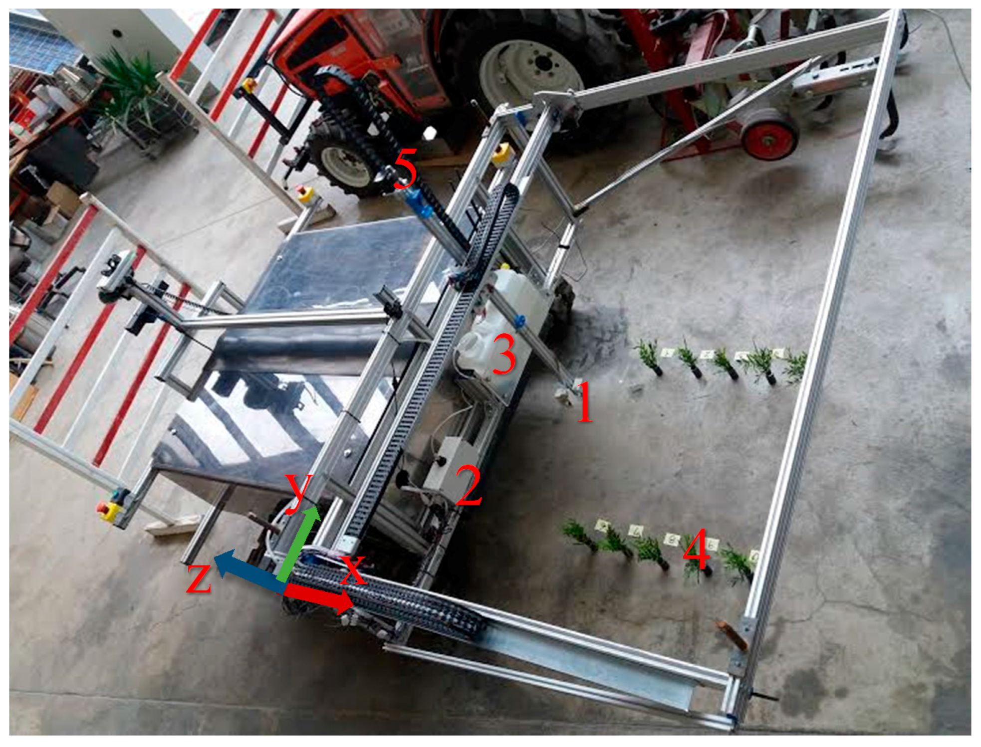
2.1. Hardware and Sensor Setup

The developed automatic system was composed of four parts: a robotic vehicle, a movable frame with three degrees of freedom, a distance-sensor and a precision spraying system. The frame mounting point for the sensor was assumed as the tool center point (TCP). The working space of the frame was 1.1 m × 1.4 m × 1.0 m (x, y, z respectively). The whole system was mounted on a field robot platform called Phoenix (developed at Hohenheim University, Stuttgart, Germany). The robot platform is able to drive 5 km/h up to a 30 degree slope and with an additional payload of 200 kg. The vehicle weighs around 450 kg. The system is driven by two electrical motors with a total power of 7 kW. The system was powered by four built-in batteries, which could provide an operation time of approximately 8–10 h, depending on driven speed, elevation and workload. The navigation computer of the robot was a Lenovo ThinkPad with i5 processor, 4 GB RAM and 320 GB disk space (Lenovo, Hong Kong, China).
As a distance sensor, a low-cost ultrasonic sensor HC-SR04 (Cytron Technologies, Johor, Malaysia) was mounted at the TCP of the frame, pointing downwards, perpendicular to the surface. The sensor had a measuring range from 2 to 400 cm and an effective angle measurement of 15 degrees. The measuring rate was limited to 10 Hz to avoid signal overlapping. The precision spraying system used a DC-Pump (Barwig GmbH, Bad Karlshafen, Germany) with a maximum supply of 22 L/min and maximum pressure of 1.4 bars. Water was used to emulate the pesticide/herbicide application, which was flowing through a plastic hose with a diameter of 10 mm that ran along the frame to the TCP. The movement of the frame axes was done through bipolar stepper motors Nema 17 (Osmtec, Ningbo, China). The stepper motors (2 for the x-axis, 1 for the y-axis, and 1 for the z-axis) had a step angle of 1.8 degrees (200 steps/revolution), a holding torque of 0.59 Nm, a step accuracy of 5% and a maximum travel speed for each axis of 0.2 m/s. The frame motors and sensors were controlled with two low-cost Raspberry Pi 2, Model B computers (Raspberry Pi Foundation, Caldecote, UK). To control the four stepper motors and the DC-Pump, three motor controllers Gertbot V 2.4 (Fen Logic Limited, Cambridge, UK) were connected to one Raspberry Pi. The sonar sensor was attached to the general purpose input/output (GPIO) pins of a second Raspberry Pi. The second Raspberry Pi was used because the attached Gertbots blocked the access to the Raspberry Pi GPIOs. Thus, using a second Raspberry Pi allowed an easier and faster implementation of the sonar sensor to the 3D frame. The whole setup of the robot with frame and plants is shown in Figure 1.

2.2. Software Setup

The control software for the robot system was programmed for the ROS-Indigo middleware (Open Source Robotics Foundation, San Francisco, CA, USA). This included the driving and navigation software of the mobile robot, as well as the control software for the frame, data acquisition of the sensors, plant detection algorithms and the precision spraying device. For visualization of the processes and acquired data, the built-in ROS 3D visualization tool “rviz” and the survey tool “rqt” were used. The driver software for the 3D frame, the pump and the motors were programmed directly on one of the Raspberry Pi computers. The sonar driver was programmed on the second Raspberry Pi. All computers were connected to the local robot network with Ethernet cables. For synchronization of all included systems and sensors of the robot and to collect the datasets, the ROS environment was installed on all systems and was used to define a synchronized time for the whole robot setup. The higher-level software was programmed on the robot navigation computer, for defining goal points and assessing the acquired data. For the point cloud assessment, parts of the Point Cloud Library (PCL) were used [39]. The Raspberry Pi operating system was Raspbian Jessie 4.1 (Raspberry Pi Foundation, Caldecote, UK) and on the navigation computer Ubuntu 14.04 (Canonical, London, England). All parts of the software were programmed in a combination of C/C++ and Python programming languages. For post processing of the recorded point clouds, Matlab R2015b (MathWorks, Natick, MA, USA) was used.

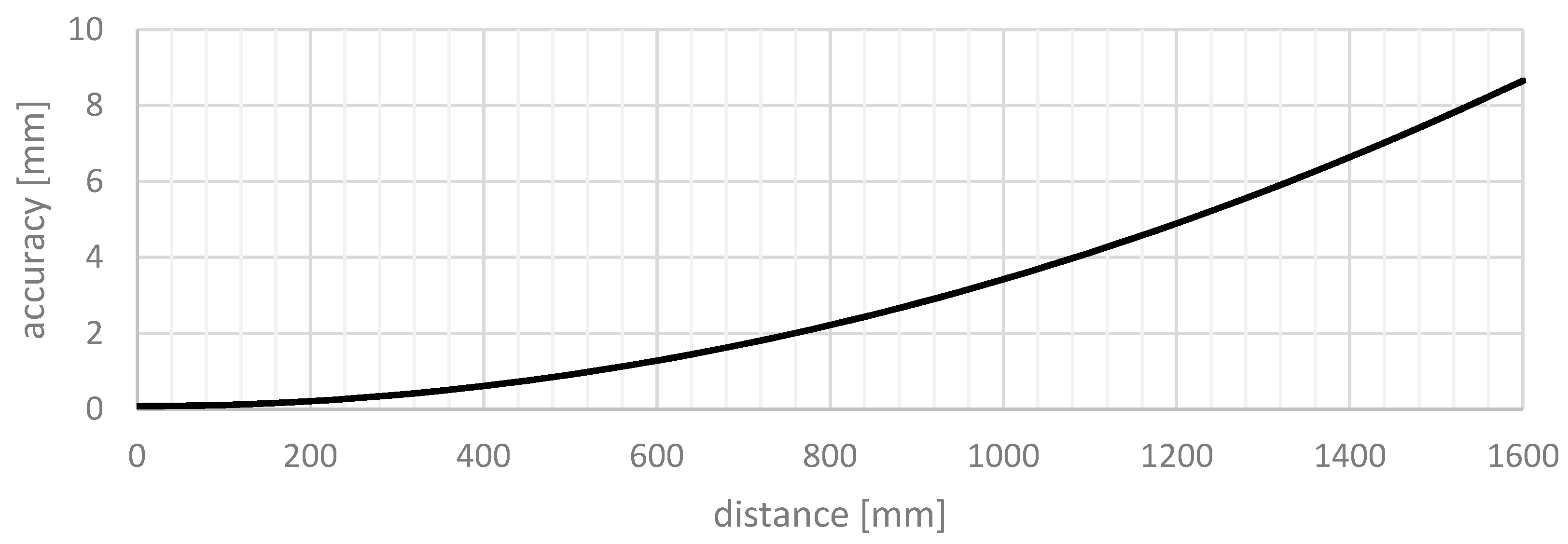
2.3. Calibration and System Test

For calibrating the frame, the relative position of the 3-axis frame was measured by a highly precise total station (SPS930, Trimble, Sunnyvale, CA, USA), together with an MT1000 tracking prism (SPS930, Trimble, Sunnyvale, CA, USA). In order to do that, the prism was attached to the highest point of the z-axis on the frame over the sonar sensor (see Figure 1). After that, the frame was moved to seven different positions inside the workspace and the relative total station output was evaluated. The measured points were spatially separated and covered the whole workspace. The total station output was compared with the moved steps of the motors and were used to define the calibration parameters of the software.
For calibrating the sonar sensor, measurements on a flat surface of a concrete floor were done and the results were compared with the movement of the z-axis. The TCP was moved downwards by the software to the relative distances of 10, 20 and 30 cm. This test was performed three times per height at different positions. All calibrations were referred to the frame coordinate system. The results were evaluated with the mean value ( d ¯ ) (1), standard deviation ( s t d d e v ) (2) and root mean square error (RMSE) (3). d i describes the distance output of the sensor, N the number of tests and d r the real value (ground truth):
d ¯ = 1 N i = 1 N d i
s t d d e v = 1 N i = 1 N ( d i d ¯ ) 2
R M S E = 1 N i = 1 N ( d i d r ) 2
The values reached by the sonar system were compared to the theoretical reachable accuracy of a stereo vision system. Stereo vision systems are quite common sensing systems for automated outdoor vehicles, making them reasonably comparable with the sonar sensor system [40]. As the accuracy of camera systems is highly affected by the object distance to the sensor position, this effect increases when using a stereo camera for 3D point cloud generation. Stereo cameras need textures in the images to find matching pixels in the two camera images, which brings a lack of distance measurements since matching is not achieved. However, if a perfect stereo camera is considered, the depth accuracy Δ Z could be described with [41]:
Δ Z = B 2 t a n ( tan 1 ( 2 Z B ) + θ ) Z
with B as baseline (distance between the two camera systems), Z as the object distance, and θ as the pixel expanding angle. θ could be described as:
θ = arctan ( p f )
with p as the pixel size and f as the focal length of the camera [41]. For comparing the two sensor principles, two different cases were considered. First, replace the sonar sensor with a stereo camera, and, second, replace the sonar sensor and the 3D frame by one fixed camera, spotting the workspace of 1.3 m × 0.9 m. As camera parameters, the values provided by Pajares et al. were used [41].

2.4. Experiment Description

The experiment was realized at the University of Hohenheim (Stuttgart, Germany) and used artificial crop plants with a height of 20 cm. To simulate the spatial separation of corn crops, the positions of the plants consisted of 2 crop rows with 5 plants each, following the seeding density for maize used by [42], with 0.75 m between each row and 0.14 m between plants. The ground truth position of each plant was measured using a pendulum attached to the TCP that was moved over the top of the plants. The software based TCP position was saved as a plant reference. Only the (x, y) coordinates were considered (see Figure 1).
To automatically detect the plants with the sonar sensor, a scan of the whole working area was first performed. The scanned route was defined to drive linearly on the field along the frame with a distance between each scanned line of 2 cm on the x-axis. The representation of a typical scan is shown in Figure 2a, where the green line is showing the planed path for the ground scanning. In addition, some tests with 2 cm × 1 cm and 2 cm × 3 cm were performed. However, the 2 cm × 2 cm resolution was used because it achieved the best results in the smallest amount of time.

2.5. Point Cloud Assembling and Processing

For each value received from the sensor, one point of the point cloud was estimated. The programmed software used different coordinate systems for each axis of the frame and was setting one coordinate system at the sensor position. The position of each axis coordinate system was estimated by the amount of steps sent to the stepper motors from the motor controllers. To estimate the precise position of a received sensor value, the transform between the sensor coordinate system and the reference coordinate system was then solved. This was possible, as the time stamp between all used controllers and sensors was synchronized. For the precise position estimation, the values were linearly interpolated. This procedure allowed for creating a spatial 3D point cloud out of the one-dimensional measurement of the sensor. To get rid of double measurements, all points in a grid with an edge length of 2 cm were filtered and summarized to one point. This led to a 3D image with a pixel size of 2 cm × 2 cm.
This 3D image was then processed to obtain the single plant positions in the considered area. First, all points belonging to the ground plane were removed, using a basic random sample consensus (RANSAC) plane algorithm [43]. The defined parameters were a maximum of 1000 iterations, sigma of 0.005 m and a distance threshold of 0.045 m. To get rid of noise, the remaining points were filtered, using a radius outlier filter (PCL 1.7.0, RadiusOutlierRemoval class). Points were considered as noise, and, when inside a radius of 0.08 m around the point, less than four additional points were found. For separating the resulting points, a kd-Tree clustering was used (PCL 1.7.0, EuclideanClusterExtraction class), assuming that the plants were separated by a gap of minimum of 0.04 m. Of each single point cloud cluster, the 3D centroid c was evaluated and assumed as the resulting plant position. With N as number of points p in the cluster (see Equation (4)),
c = 1 N i = 1 n p i
The resulting plant positions of the algorithm were compared with the ground truth to obtain the precision. The assembled point cloud and the detected plant positions could be visualized in real-time with the help of the ROS visualization tool “rviz” (see Figure 2b).

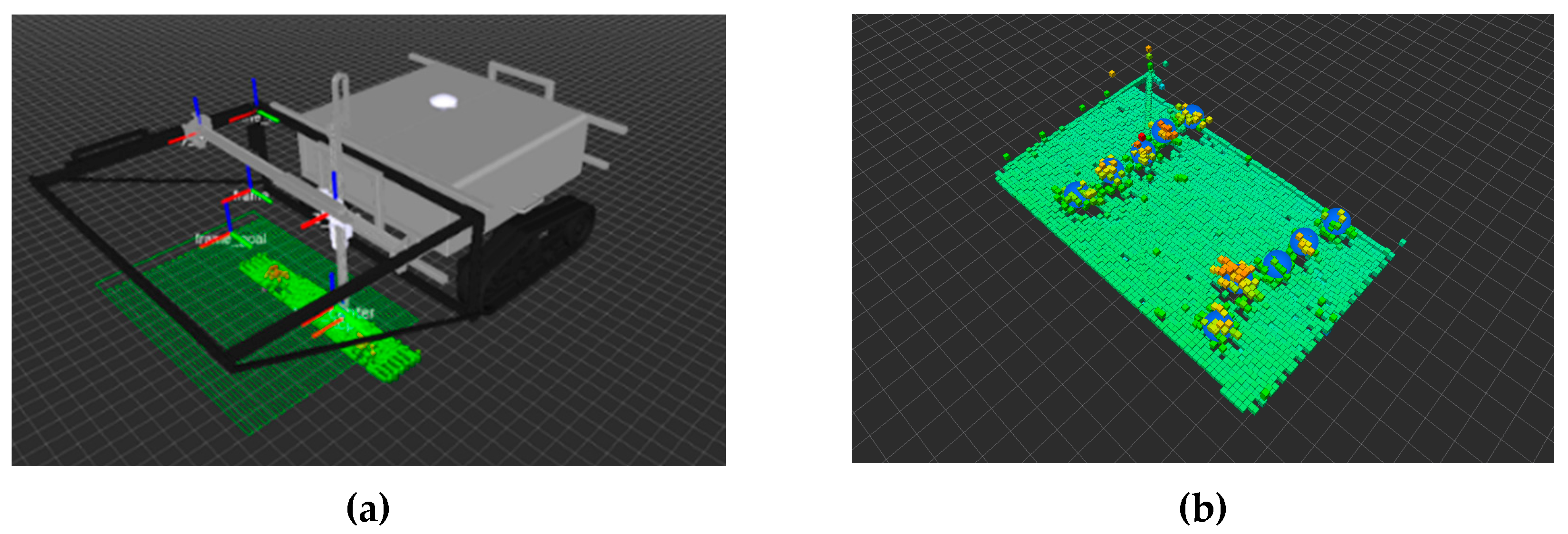
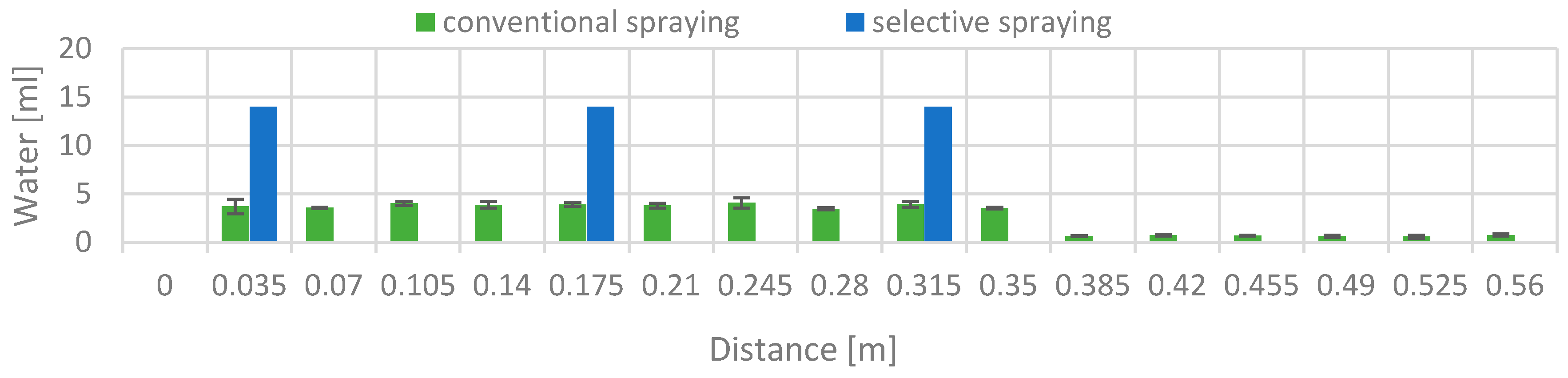
2.6. Precision Spraying

The plant coordinates were extracted automatically from the point cloud, and, subsequently, could be used for the implementation of the automatic spraying algorithm. The coordinates were sent as goals to the frame motor driver board, and the programmed goal manager activated the pump as soon as the goal was reached. Because of the linear shift between the sonar sensor and pump exit point, a static translation was applied to the plant positions with a 3 cm x-axis and a 4 cm y-axis. Two spraying configurations were applied for the comparison of the saved liquid. The first method was a continuous application along the plant rows (conventional spraying). The second method applied the liquid spray at the estimated plant position (selective spraying). The pump was turned on, for the first method, when the first plant position was reached in a distance range of +/− 2 cm, while, for the second, the pump was turned on when the estimated plant position was reached with a precision of +/− 1 mm. This procedure was performed with three replicates, in which the amount of liquid applied in each test was quantified with small canisters with a diameter of 35 mm, placed under the application points. In total, 17 canisters were placed in a row, covering a distance of 0.56 m. For both methods, 42 mL were used. With the conventional method, the amount of water was applied over the whole line, while, with the selective method, the frame was moving to the plant poses and was applying the water (14 mL per plant). The three plant poses were assumed to be at the x-axis positions 0.035, 0.175 and 0.315 m, separated by a spacing of 14 cm.

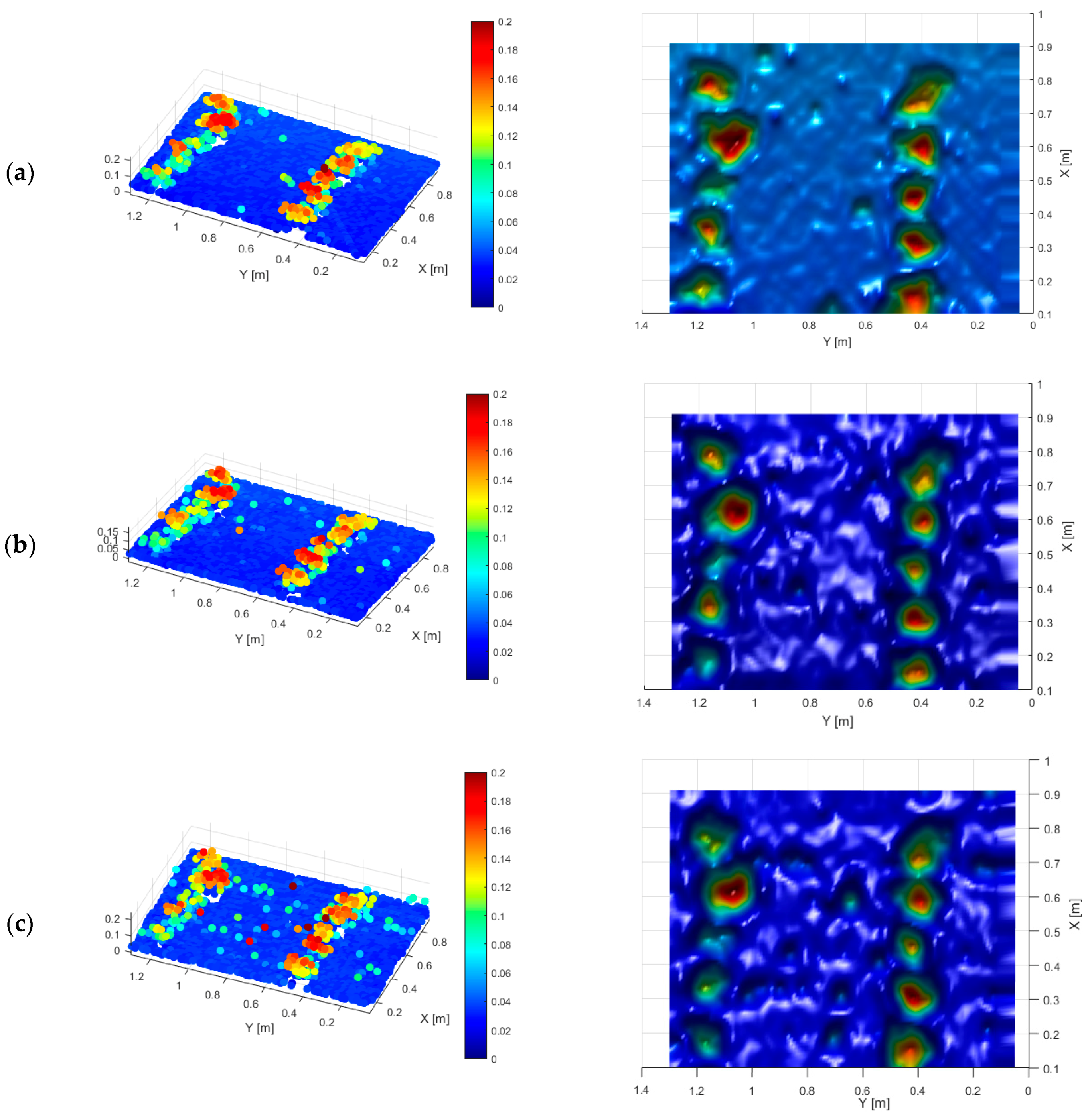
3. Results and Discussion

After the calibration of the TCP with the help of the total station, the measured positions of the frame showed results of +/− 1 mm deviation between the software estimated positions and the total station. This precision was achievable for two relative points. The system was able to recalibrate itself by driving once again to the end stop position at the edges of the working range. This allowed relocating the same position with the same precision inside the working range of the frame, as long as the mobile robot system was not moving. As soon as the system was starting and stopping several times without reaching an end stop, the position error accumulated. This was caused by the mechanical inertia while stopping the system, as a consequence generating a slight slipping of the axis. For testing the limits of the system, the seven points were approached, without returning to the next end stop. The details of the performed test points are described in the following Table 1. Because of the accumulation of the errors, the precision for the y-axis got an absolute precision deviation of 4 mm. The highest measurement error was 0.32%, compared to the distance. It could be assumed that the system is able to collect spatial referenced sensor data in the millimeter range. This level of precision was obtained thanks to the controllable discrete angular displacement engines, whose high resolution and precise steps played a significant role in the overall accuracy of the positioning system.
Regarding the calibration of the ultrasonic sensor, the height detected by the ultrasonic sensor and vertical movement of the TCP was compared. It indicated a variable precision of the system depending on the height of the sensor. This precision decreased as the distance was reduced to the measured object, with an RMSE of 5.5 mm for 10 cm, going down to 0.2 mm at a height above 30 cm (see Table 2). The maximum standard deviation was 4.1 mm and the minimal was at the 30 cm point at 0.2 mm. For this reason, the detection of plants (with an average height of 20 cm) was performed at a height of 40 cm from the ground, thus avoiding an increase in measurement error.
For assessing the accuracy of a theoretical stereo vision system as a possible replacement for the sonar sensor, a baseline of 30 cm, a focal length of 10 mm and a camera pixel size of 5 µm as described by Pajares et al. were assumed. When solving Equations (4) and (5) with these parameters and a variable object distance, the theoretical depth accuracy could be described with the following graph (see Figure 3). To compare the values, the absolute values were also included in Table 2 below for the estimated height poses of 10, 20 and 30 cm.
It is evident that 3D visual system accuracy is highly dependent on the object distance. Therefore, it could be seen that the sonar sensor is less precise than the stereo system at short distances (10 cm) but already performs better when the object is placed at a 30 cm distance. This means that the advantage of a stereo camera is not at the depth accuracy, compared to a sonar sensor, but by the spatial resolution. Instead of mounting the camera at the TCP, the stereo camera could also be mounted in a fixed position to monitor the complete workspace of 1.3 m × 0.9 m at once. By using a typical camera angle of view of 50 degrees, this would lead to a necessary mounting height of at least 1.39 m, which would lead to an accuracy of 6.58 mm.
This would increase the error compared to the used low-cost sonar system. As the accuracy of stereo cameras is effected by sunlight, light reflections, lack of texture or light (night) and the used matching algorithm [44], this accuracy could get worse under real field conditions, which would not be the case with sonar sensors.
To increase the accuracy of the system and to minimize the influence of the accumulation of path errors (see Table 1), the sonar scans of the 3D frame were separated into 10 small segments of 10 cm × 140 cm. After each segment, the frame was driven to one end stop. The total time for each scan was 10 min. The unfiltered representation of the experimental area contained a total of 3801, 4383 and 4469 points for the three scans performed. After filtering the scan area to one point for each grid of 2 cm × 2 cm, the resulting points for the three scans were 2931, 2906 and 2907 points. The results of the point clouds are shown in Figure 4. Only points in the x-axis and y-axis greater than 0.1 m were considered. The 3D point representation is shown on the left side. The right picture depicts the same data as the surface reconstruction. The value of every grid was extrapolated by smoothing the values with the given point cloud dataset using a Delaunay triangulation principle with the use of the Matlab function gridfit [45]. The showed graphs were solved by setting a grid size of 1 cm over the considered area, defining a smoothing factor of 2 for the dataset.
Out of the generated 3D point clouds, it is possible to observe the plant positions represented by the higher altitudes. Around the center of the plant, the height formed the maximum with a balloon like shape. When reconstructing a surface out of the 3D point cloud (see Figure 4), the peaks are strongly correlated with the real plant position, which leads to the assumption that the peaks are also the real plant center positions. However, the reflections of leaves caused points to overlap, making the clusters of the single plants harder to separate. In addition, some plants were detected better than others, where the morphology of each plant could be a cause. The difference in height between plants was, in some cases, more than 10 cm. However, there was always a detectable peak for every single plant.
The applied algorithm for the single plant detection needed a clear spacing between the points to cluster the plants. In this described case, the distance between the plants was set to 0.14 m. This distance was sufficient to estimate a clear spacing between the plants, leading to an automatic performed plant detection rate of 100% in all performed scans.
Obtaining the coordinates of each plant was done in real time by the described algorithm. The 3D centroid of each cluster was assumed as the plant position. However, the actual center of the plant varied depending on the orientation of the leaves, their density, size and height. This caused the center of the cluster to not exactly match the real plant origin, but represented the center of the plant’s leaf area, which triggers advantages for autonomous spraying, as the leaves are normally the areas of interest.
Figure 5 shows a comparison between the pendulums measured, coordinates of the plant centers, and the coordinates obtained from the point clouds. The average distance of the plants to the real position was 2.4 cm in the (x, y) coordinates with an RMSE of 2.7 cm. This gives the system a good precision considering the influence of the leaf area on the determination of the location of the plants and the systems’ TCP movement.
Therefore, it was assumed that the system is capable of obtaining the location of plants without prior measurements of their actual location when the following conditions are fulfilled:
  • The ground surface must have a planar shape so that it can be detected with a RANSAC plane-fitting algorithm. The soil irregularities must be smaller than the height of the plants.
  • The plant leaves should not cover the area between the plants, so that height differences at the plant gaps are detectable.
  • No other sonar sources should interfere with the sensor system.
  • The plant height is smaller than approximately 0.5 m, since the TCP or the mobile robot could touch the leaves, producing incorrect measurements or damaging the plants.
As the sensor system is not affected by sunlight, it could be assumed that the sensor detection will also perform well under outdoor field conditions, when the monitored environment is similar to the tested experiment, with a planar like soil surface and spatially separated plants. One advantage of the used sonar sensor, compared to other sensor types, is that, inside the measurement cone, the highest value is reflected back. Therefore, since the closest point is reflected, a low image resolution can be generated without missing the high peaks of a region. However, the spatial resolution of the sensor hardly allows the detection of small plant details like single leaves. On the other hand, with a LiDAR system, it would be easy to miss the highest spot of a plant when the measurement resolution is too low. Consequently, sonar sensors could help to create robust 3D imaging methods for precision spraying and plant height estimation.
However, when using the sensor system for outdoor field testing, the main influence factor on the results is assumed to be the change of the surface structure. In particular, the roughness of the soil could cause measurement errors. As sonar sensors are not able to detect flat surfaces with a higher inclination to the sensor, this could cause measurement errors in rough terrain. The same problem could occur when plants form sharp edges. Wind could change the surface while scanning, leading to moving plant leaves that could result in incorrectly aligned plant positions or measurement noise. The measurement quality will not change with sonar sensors under changing weather conditions in general, as is typical with vision based sensor systems, so that shading of the sensors must not be considered.
As previously mentioned, it was found that planting distances significantly affect the formation of clusters. Close proximity between plants caused corresponding plant points to not be able to be separated, and two plants were considered as one. In the described experiment, the plant spacing was set to 14 cm, which was adequate for identifying all the plants without causing overlaps or unifications of clusters. As long as the plants show a height difference between their gaps and do not completely overlap, the plants can then be detected and clustered.
For comparing selective to conventional spraying, six tests were performed in total. The measured values were averaged for every canister with the spacing of 0.035 m and the results were compared. The results are shown in Figure 6 below.
The standard deviations of the measured liquid content of the performed experiments were between 0.754 and 0.042 mL. The selective method applied all water spray precisely on the single plants, without any loss in the canisters of 3.5 cm diameter. The results of the continuous spraying showed a constant distribution over the measured area. The water distribution showed a continuous application of approximately 4 mL in the first 0.35 m of the path. However, the value was decreased to values close to 0.8 mL the rest of the way. This phenomenon was generated because the pump did not provide a continuous pressure or a shut off valve to keep the liquid inside the hose. In the selective application, no liquid was lost, as the TCP was not moving while the pump was working.
When comparing the amount of water applied at the plant pose canister, the selective spraying method applied on average 3.6 times more water to the plants than the conventional method. With the conventional method, a total of 151.2 mL must be applied so that the plant obtains the same amount of water. This would represent a savings of 109.2 mL or 72% of the conventional spraying method.
Similar values were reported by [10,12,17,46], who gave a pesticide reduction of 34.5%, 58%, 64% and 66%, respectively, when compared to a conventional homogeneous spraying. The result of these tests confirmed that an inexpensive precision system could confer significant reductions in the use of herbicides.
The main disadvantage of the proposed method is the low speed. As the actual scanning time of the workspace needs around 10 min for 10 plants, a performance of 1 min per plant would lead from a density of nine plants per square meter [42] to a performance of approximately 166 h per hectare.
This means that, for real-time applications, scanning with a sonar sensor at the TCP is not promising. A fixed 2D array of sonar sensors spaced within a few centimeters, using the robot movement to create a spatial 3D image, would be much faster. When this is combined with a movable spray nozzle per row, the speed could be adjusted depending on the required sonar sensor grid size. With a grid size of 2 cm and the used 10 Hz of the sonar sensor, the driving speed of the sonar sensor, the system could cover 1.3 m2 in 5 s, which leads to approximately 10 h per hectare. With a robotic system working 24 h a day, this could already have a good cost benefit ratio. The 3D image obtained by the system could even be used to spray according to the measured canopy volume of the 3D image to apply the liquid more effectively. In addition, the use of a magnet valve would help to apply the liquid more precisely to the plants.
Future work should also include research in real outdoor conditions, in order to define the minimal necessary grid size of the sensor readings to be quick without missing useful information. To understand the advantages of different sensor systems, it could also help to compare the differences between the use of a LiDAR sensor and a sonar sensor, comparing detection rate, precision and possible speed for detecting single plants. For more robust plant detection, other clustering algorithms like a k-means or graph-cut based principles could be investigated.

4. Conclusions

An autonomous selective spraying robot was developed and tested at the University of Hohenheim. This system was composed by a mobile robot with a mounted frame with three degrees of freedom. An ultrasonic sensor was mounted at the frame TCP to scan the surface with the aim of determining the height of the objects inside the working range. The precision of the horizontal movement of the TCP was determined with +/− 1 mm. The vertical precision depended on the height measurement of the ultrasonic sensor. The ultrasonic sensor RMSE was between 5.5 to 0.2 mm, depending on the distances between the objects and the sensor. The 3D position of the TCP was fused with the sonar sensor value to generate a 3D point cloud.
Three scans were performed, finding on average a total of 4127 points per scan. This point cloud allowed differing plants to be present in the scanning area. To acquire the exact plant positions, the ground points were removed by a RANSAC plane-fitting algorithm. The resulting points were separated with a Euclidian distance clustering. The centroid of each cluster represented the estimated plant position. The estimation of the plant coordinates demonstrated an RMSE of 2.7 cm, allowing a real-time location and spraying of the position by an attached control valve at the TCP. This would be sufficient to detect single plant structures and allow single plant treatment. The comparative tests between the selective spraying method and the conventional spraying in this investigation showed that, with the reduction of the amount of the spraying operation in places where it is not necessary, savings of about 72% could be provided.
The sonar sensor allows variable grid sizes and is not affected by sunlight, leading to the assumption that it could perform well in outdoor conditions. From an economic and environmental point of view, the designed system could provide ideas for low-cost precision spraying by reducing soil and groundwater contamination. Therefore, it could decrease the use of herbicides, workers and working time.

Acknowledgments

The project was conducted at the Max Eyth Endowed Chair (Instrumentation and Test Engineering) at Hohenheim University (Stuttgart, Germany), which is a partial grant funded by the Deutsche Landwirtschafts-Gesellschaft e.V. (DLG).

Author Contributions

The experiment planning and the programming of the software was done by David Reiser, Javier M. Martín-López and Emir Memic. The writing was performed by David Reiser and Javier M. Martín-López. The experiments, the analysis and processing of the data were conducted by David Reiser, Javier M. Martín-López and Emir Memic. The mechanical development and design of the frame was performed by Manuel Vázquez-Arellano and Steffen Brandner. The whole experiment was supervised by Hans W. Griepentrog.

Conflicts of Interest

The authors declare no conflict of interest.

References

  1. El-Gawad, H.A. Validation method of organochlorine pesticides residues in water using gas chromatography—Quadruple mass. Water Sci. 2016, 30, 96–107. [Google Scholar] [CrossRef]
  2. Gaillard, J.; Thomas, M.; Iuretig, A.; Pallez, C.; Feidt, C.; Dauchy, X.; Banas, D. Barrage fishponds: Reduction of pesticide concentration peaks and associated risk of adverse ecological effects in headwater streams. J. Environ. Manag. 2016, 169, 261–271. [Google Scholar] [CrossRef] [PubMed]
  3. Oerke, E.-C. Crop losses to pests. J. Agric. Sci. 2006, 144, 31. [Google Scholar] [CrossRef]
  4. Kira, O.; Linker, R.; Dubowski, Y. Estimating drift of airborne pesticides during orchard spraying using active Open Path FTIR. Atmos. Environ. 2016, 142, 264–270. [Google Scholar] [CrossRef]
  5. Doulia, D.S.; Anagnos, E.K.; Liapis, K.S.; Klimentzos, D.A. Removal of pesticides from white and red wines by microfiltration. J. Hazard. Mater. 2016, 317, 135–146. [Google Scholar] [CrossRef] [PubMed]
  6. Heap, I. Global perspective of herbicide-resistant weeds. Pest Manag. Sci. 2014, 70, 1306–1315. [Google Scholar] [CrossRef] [PubMed]
  7. Alves, J.; Maria, J.; Ferreira, S.; Talamini, V.; De Fátima, J.; Medianeira, T.; Damian, O.; Bohrer, M.; Zanella, R.; Beatriz, C.; et al. Determination of pesticides in coconut (Cocos nucifera Linn.) water and pulp using modified QuEChERS and LC–MS/MS. Food Chem. 2016, 213, 616–624. [Google Scholar]
  8. Solanelles, F.; Escolà, A.; Planas, S.; Rosell, J.R.; Camp, F.; Gràcia, F. An Electronic Control System for Pesticide Application Proportional to the Canopy Width of Tree Crops. Biosyst. Eng. 2006, 95, 473–481. [Google Scholar] [CrossRef]
  9. Chang, J.; Li, H.; Hou, T.; Li, F. Paper-based fluorescent sensor for rapid naked-eye detection of acetylcholinesterase activity and organophosphorus pesticides with high sensitivity and selectivity. Biosens. Bioelectron. 2016, 86, 971–977. [Google Scholar] [CrossRef] [PubMed]
  10. Gonzalez-de-Soto, M.; Emmi, L.; Perez-Ruiz, M.; Aguera, J.; Gonzalez-de-Santos, P. Autonomous systems for precise spraying—Evaluation of a robotised patch sprayer. Biosyst. Eng. 2016, 146, 165–182. [Google Scholar] [CrossRef]
  11. Peteinatos, G.G.; Weis, M.; Andújar, D.; Rueda Ayala, V.; Gerhards, R. Potential use of ground-based sensor technologies for weed detection. Pest Manag. Sci. 2014, 70, 190–199. [Google Scholar] [CrossRef] [PubMed]
  12. Oberti, R.; Marchi, M.; Tirelli, P.; Calcante, A.; Iriti, M.; Tona, E.; Ho, M.; Pfaff, J.; Schu, C. Selective spraying of grapevines for disease control using a modular agricultural robot. Biosyst. Eng. 2016, 146, 203–215. [Google Scholar] [CrossRef]
  13. Slaughter, D.C.; Giles, D.K.; Downey, D. Autonomous robotic weed control systems: A review. Comput. Electron. Agric. 2008, 61, 63–78. [Google Scholar] [CrossRef]
  14. Blackmore, B.S.; Griepentrog, H.W.; Fountas, S. Autonomous Systems for European Agriculture. In Proceedings of the Automation Technology for Off-Road Equipment, Bonn, Germany, 1–2 September 2006.
  15. Lee, W.S.; Slaughter, D.C.; Giles, D.K. Robotic weed control system for tomatoes. Precis. Agric. 1999, 1, 95–113. [Google Scholar] [CrossRef]
  16. Kunz, C.; Sturm, D.J.; Peteinatos, G.G.; Gerhards, R. Weed suppression of Living Mulch in Sugar Beets. Gesunde Pflanz. 2016, 68, 145–154. [Google Scholar] [CrossRef]
  17. Gil, E.; Escolà, A.; Rosell, J.R.; Planas, S.; Val, L. Variable rate application of Plant Protection Products in vineyard using ultrasonic sensors. Crop Prot. 2007, 26, 1287–1297. [Google Scholar] [CrossRef]
  18. Garrido, M.; Paraforos, D.; Reiser, D.; Vázquez Arellano, M.; Griepentrog, H.; Valero, C. 3D Maize Plant Reconstruction Based on Georeferenced Overlapping LiDAR Point Clouds. Remote Sens. 2015, 7, 17077–17096. [Google Scholar] [CrossRef]
  19. Woods, J.; Christian, J. Glidar: An OpenGL-based, Real-Time, and Open Source 3D Sensor Simulator for Testing Computer Vision Algorithms. J. Imaging 2016, 2, 5. [Google Scholar] [CrossRef]
  20. Backman, J.; Oksanen, T.; Visala, A. Navigation system for agricultural machines: Nonlinear Model Predictive path tracking. Comput. Electron. Agric. 2012, 82, 32–43. [Google Scholar] [CrossRef]
  21. Berge, T.W.; Goldberg, S.; Kaspersen, K.; Netland, J. Towards machine vision based site-specific weed management in cereals. Comput. Electron. Agric. 2012, 81, 79–86. [Google Scholar] [CrossRef]
  22. Bietresato, M.; Carabin, G.; Vidoni, R.; Gasparetto, A.; Mazzetto, F. Evaluation of a LiDAR-based 3D-stereoscopic vision system for crop-monitoring applications. Comput. Electron. Agric. 2016, 124, 1–13. [Google Scholar] [CrossRef]
  23. Vázquez-Arellano, M.; Griepentrog, H.W.; Reiser, D.; Paraforos, D.S. 3-D Imaging Systems for Agricultural Applications—A Review. Sensors 2016, 16, 24. [Google Scholar] [CrossRef] [PubMed]
  24. Andújar, D.; Dorado, J.; Fernández-Quintanilla, C.; Ribeiro, A. An approach to the use of depth cameras for weed volume estimation. Sensors 2016, 16, 1–11. [Google Scholar] [CrossRef] [PubMed]
  25. Jiang, Y.; Li, C.; Paterson, A.H. High throughput phenotyping of cotton plant height using depth images under field conditions. Comput. Electron. Agric. 2016, 130, 57–68. [Google Scholar] [CrossRef]
  26. Kusumam, K.; Kranjík, T.; Pearson, S.; Cielniak, G.; Duckett, T. Can You Pick a Broccoli? 3D-Vision Based Detection and Localisation of Broccoli Heads in the Field. In Proceedings of the IEEE International Conference on Intelligent Robots and Systems, Deajeon, Korea, 9–14 October 2016; pp. 1–6.
  27. Tumbo, S.D.; Salyani, M.; Whitney, J.D.; Wheaton, T.A.; Miller, W.M. Investigation of Laser and Ultrasonic Ranging Sensors for Measurements of Citrus Canopy Volume. Appl. Eng. Agric. 2002, 18, 367–372. [Google Scholar] [CrossRef]
  28. Giles, D.K.; Delwiche, M.J.; Dodd, R.B. Control of orchard spraying based on electronic sensing of target characteristics. Trans. ASABE 1987, 30, 1624–1630. [Google Scholar] [CrossRef]
  29. Doruchowski, G.; Holownicki, R. Environmentally friendly spray techniques for tree crops. Crop Prot. 2000, 19, 617–622. [Google Scholar] [CrossRef]
  30. Swain, K.C.; Zaman, Q.U.Z.; Schumann, A.W.; Percival, D.C. Detecting weed and bare-spot in wild blueberry using ultrasonic sensor technology. Am. Soc. Agric. Biol. Eng. Annu. Int. Meet. 2009 2009, 8, 5412–5419. [Google Scholar]
  31. Zaman, Q.U.; Schumann, A.W.; Miller, W.M. Variable rate nitrogen application in Florida citrus based on ultrasonically-sensed tree size. Appl. Eng. Agric. 2005, 21, 331–335. [Google Scholar] [CrossRef]
  32. Walklate, P.J.; Cross, J.V.; Richardson, G.M.; Baker, D.E. Optimising the adjustment of label-recommended dose rate for orchard spraying. Crop Prot. 2006, 25, 1080–1086. [Google Scholar] [CrossRef]
  33. Reiser, D.; Paraforos, D.S.; Khan, M.T.; Griepentrog, H.W.; Vázquez Arellano, M. Autonomous field navigation, data acquisition and node location in wireless sensor networks. Precis. Agric. 2016, 1, 1–14. [Google Scholar] [CrossRef]
  34. Zlot, R.; Bosse, M. Efficient Large-scale Three-dimensional Mobile Mapping for Underground Mines. J. Field Robot. 2014, 31, 758–779. [Google Scholar] [CrossRef]
  35. Reiser, D.; Izard, M.G.; Arellano, M.V.; Griepentrog, H.W.; Paraforos, D.S. Crop Row Detection in Maize for Developing Navigation Algorithms under Changing Plant Growth Stages. In Advances in Intelligent Systems and Computing; Springer: Lisbon, Portugal, 2016; Volume 417, pp. 371–382. [Google Scholar]
  36. Weiss, U.; Biber, P. Plant detection and mapping for agricultural robots using a 3D LIDAR sensor. Robot. Auton. Syst. 2011, 59, 265–273. [Google Scholar] [CrossRef]
  37. Back, W.C.; van Henten, E.J.; Edan, Y. Harvesting Robots for High-value Crops: State-of-the-art Review and Challenges Ahead. J. Field Robot. 2014, 31, 888–911. [Google Scholar] [CrossRef]
  38. Dornbusch, T.; Wernecke, P.; Diepenbrock, W. A method to extract morphological traits of plant organs from 3D point clouds as a database for an architectural plant model. Ecol. Modell. 2007, 200, 119–129. [Google Scholar] [CrossRef]
  39. Rusu, R.B.; Cousins, S. 3D is here: Point cloud library. In Proceedings of the 2011 IEEE International Conference on Robotics and Automation (ICRA), Shanghai, China, 9–13 May 2011; pp. 1–4.
  40. Rovira-Más, F.; Wang, Q.; Zhang, Q. Design parameters for adjusting the visual field of binocular stereo cameras. Biosyst. Eng. 2010, 105, 59–70. [Google Scholar] [CrossRef]
  41. Pajares, G.; García-Santillán, I.; Campos, Y.; Montalvo, M.; Guerrero, J.; Emmi, L.; Romeo, J.; Guijarro, M.; Gonzalez-de-Santos, P. Machine-Vision Systems Selection for Agricultural Vehicles: A Guide. J. Imaging 2016, 2, 34. [Google Scholar] [CrossRef]
  42. Reckleben, Y. Cultivation of maize—Which sowing row distance is needed? Landtechnik 2011, 66, 370–372. [Google Scholar]
  43. Fischler, M.A.; Bolles, R.C. Random Sample Consensus: A Paradigm for Model Fitting with Applications to Image Analysis and Automated Cartography. Commun. ACM 1981, 24, 381–395. [Google Scholar] [CrossRef]
  44. Hirschmüller, H. Stereo processing by semiglobal matching and mutual information. IEEE Trans. Pattern Anal. Mach. Intell. 2008, 30, 328–341. [Google Scholar] [CrossRef] [PubMed]
  45. Errico, J.D. Matlab Gridfit Function. Available online: https://de.mathworks.com/matlabcentral/fileexchange/8998-surface-fitting-using-gridfit (accessed on 23 December 2016).
  46. Maghsoudi, H.; Minaei, S.; Ghobadian, B.; Masoudi, H. Ultrasonic sensing of pistachio canopy for low-volume precision spraying. Comput. Electron. Agric. 2015, 112, 149–160. [Google Scholar] [CrossRef]
Figure 1. Description of the used automatic spraying system with all the hardware components mounted (1. Tool center point; 2. Control unit and motor controllers; 3. Water tank; 4. Plants; 5. Calibration point).
Jimaging 03 00009 g001
Figure 2. Visualization of the robot system (a) and the acquired point cloud in ROS-rviz, with the estimated plant positions by the software algorithm (blue dots) (b).
Jimaging 03 00009 g002
Figure 3. Development of the accuracy of a stereo vision system, with the assumed parameters B = 300 mm, f = 10 mm and p = 5 µm (see Equations (4) and (5)).
Jimaging 03 00009 g003
Figure 4. Visualization of the received 3D point clouds and surface reconstructions for the three scans (ac). All readings are in m.
Jimaging 03 00009 g004
Figure 5. Estimated plant poses in x and y—with the ground truth (x) and the results for the three scans (*, o, +).
Jimaging 03 00009 g005
Figure 6. Average distribution of the conventional spraying compared to the selective spraying with two standard deviations.
Jimaging 03 00009 g006
Table 1. List of the performed calibration points with results.
No.Total Station Measurement (m)Software Position (m)
xyxy
10.0000.0000.0000.000
20.0001.0010.0001.000
30.0011.4590.0001.460
40.4990.4960.5000.500
50.5001.4560.5001.460
61.0000.0051.0000.000
71.0001.4551.0001.460
Table 2. Calibration results of the sonar sensor compared with the accuracy of a theoretical stereo camera.
Estimated Pose (m)Measured Sonar Value (m)Stereo Camera (m)
d ¯ s t d d e v RMSEAccuracy
0.10000.10370.00410.00550.00011
0.20000.20370.00190.00410.00021
0.30000.30010.00020.00020.00038

