3D Reconstructions Using Unstabilized Video Footage from an Unmanned Aerial Vehicle


1
Urban Modelling Group, UCD School of Civil Engineering, University College Dublin, Newstead, Belfield, Dublin 4, Ireland
2
UCD School of Computer Science and Informatics, University College Dublin, Belfield, Dublin 4, Ireland
3
UCD Earth Institute, Richview, Belfield, Dublin 4, Ireland
4
Center for Urban Science and Progress, New York University, 1 MetroTech Center, Brooklyn, NY 11201, USA
*
Author to whom correspondence should be addressed.
J. Imaging 2017, 3(2), 15; https://doi.org/10.3390/jimaging3020015
Submission received: 31 January 2017
/
Revised: 12 April 2017
/
Accepted: 18 April 2017
/
Published: 22 April 2017
(This article belongs to the Special Issue Big Visual Data Processing and Analytics)
Abstract
:Structure from motion (SFM) is a methodology for automatically reconstructing three-dimensional (3D) models from a series of two-dimensional (2D) images when there is no a priori knowledge of the camera location and direction. Modern unmanned aerial vehicles (UAV) now provide a low-cost means of obtaining aerial video footage of a point of interest. Unfortunately, raw video lacks the required information for SFM software, as it does not record exchangeable image file (EXIF) information for the frames. In this work, a solution is presented to modify aerial video so that it can be used for photogrammetry. The paper then examines how the field of view effects the quality of the reconstruction. The input is unstabilized, and distorted video footage obtained from a low-cost UAV which is then combined with an open-source SFM system to reconstruct a 3D model. This approach creates a high quality reconstruction by reducing the amount of unknown variables, such as focal length and sensor size, while increasing the data density. The experiments conducted examine the optical field of view settings to provide sufficient overlap without sacrificing image quality or exacerbating distortion. The system costs less than €1000, and the results show the ability to reproduce 3D models that are of centimeter-level accuracy. For verification, the results were compared against millimeter-level accurate models derived from laser scanning.
1. Introduction
The global market for unmanned aerial vehicles (UAV) is currently worth €5.4 billion and is expected to grow to €6.35 billion by 2018 [1]. A significant area of expansion has been in the micro-UAV sector where units weigh less than 1 kg. Over the past five years, there has been a dramatic increase in options in micro-UAV models coupled with significant price reductions and notable capacity enhancements [2]. A UAV costing €500 may now be equipped with accelerometers, magnetometers, barometers and global positioning system (GPS) locators [3]. These capabilities allow for automatic three-axis stabilization and relative direction control. A decade ago, such a system would only have been available as a high-end, bespoke system and would have been orders of magnitude more costly. Today, many of these systems come with an on-board camera (e.g., Parrot AR drone) or can be fitted with a lightweight one (e.g., DJI Phantom, Blade QX). Accordingly, obtaining aerial imagery of a site of interest with an inexpensive UAV flown by a relatively inexperienced user is much more feasible. These units can now facilitate a new pipeline for three-dimensional (3D) model reconstruction by supporting aerial video footage capture.
Aerial footage generates the opportunity to construct 3D models from 2D input. A technique called structure from motion (SFM) makes this possible by combining feature extraction, point matching and existing knowledge of the vision system. Traditionally, SFM has been undertaken either with only a limited number of images or using costly commercial software such as Agisoft Photoscan [4] to combine large numbers of images. Today, however, open-source SFM packages are available. Software packages such as OpenMVG [5] and VisualSFM [6] offer the potential for the free and fast processing of thousands of images and produce results comparable to commercial software.
SFM is a fully-automatic procedure that uses several computer vision techniques and feature detection algorithms to simultaneously solve the 3D structure of a scene and the viewing parameters to recreate a 3D model. It allows for low-cost surveys to be conducted, which makes it possible to do multi-temporal surveys [7]. While SFM techniques are automatic, they are not infallible. Extreme changes in light, rapid movements, or unknown camera parameters complicate reconstruction activities. Specifically, SFM requires sufficient commonality between images to allow for point matching. The amount of overlap between images affects the likelihood of finding a match and, thus, making a reconstruction possible.
The extent of overlap can be increased by collecting a greater number of images to be used as input. This can be accomplished in three ways: (1) using multiple UAVs; (2) flying multiple missions; or (3) capturing a greater quantity of images in a single flight, as exemplified by video footage. Due to the decreasing cost of robotics, there is active research into collaborative exploration of an environment. Robots operating on smart phone technology can collaborate over the cloud [8] in order to collect the necessary data to build a model of the environment. Formation flight by multiple UAVs [9] is now possible and would allow a much greater area to be covered by a team of UAVs flying simultaneously.
In this work, the third option is taken to increase overlap by capturing more images with a single UAV by using video-based photogrammetry (videogrammetry). While too much overlap can reduce the accuracy of the reconstruction, the ability to increase overlap by pulling more frames from the video allows unstabilized and highly kinetic footage to be used in reconstructions. To date, videogrammetry is predominantly applied in robotics [10] and industrial manufacturing [11] and has not yet been extensively applied to mapping. This work shows how video footage can be combined with an SFM system to build an accurate 3D model to represent an element in the built environment.
In addition to increasing the number of input images, image overlap can be improved by capturing a larger section of the target scene in each image. Previous work (e.g., [12]) in this area has shown that increasing the distance from the target can improve the final results. A larger portion of the target area can also be collected without altering the distance, but instead by changing the camera’s field of view (FOV).
This work was born out of a requirement for low-cost aerial imagery of sufficient quality and coverage to generate a 3D model for surveying work and to examine what field of view setting generates the most accurate results. Initially, the paper describes an approach that allows video footage from a low-cost camera with significant lens distortion to be used to generate 3D models. Although the footage was obtained using a UAV, this could be done with any low-cost camera system. The main focus of this work, however, is to examine how changing the FOV, and hence the level of distortion, affects the 3D model output. The results show that although distortion can affect the accuracy of the model, the increased FOV makes it easier for SFM to generate a 3D model, as it furnishes a greater area in each image for keypoint detection.
2. Methods and Materials
SFM reconstructs a 3D model from a sequence of images without a priori knowledge of the camera pose (location, orientation and field of view). Although it uses several modern techniques for keypoint detection and dense reconstruction, it also borrows methods developed for classic photogrammetry, such as self-calibrating bundle adjustment [13], to automatically estimate the camera pose.
The SFM process steps are as follows: (1) feature detection; (2) alignment; (3) bundle adjustment; and (4) reconstruction. The open source software VisualSFM was used in this work, the specifics of which are described below.
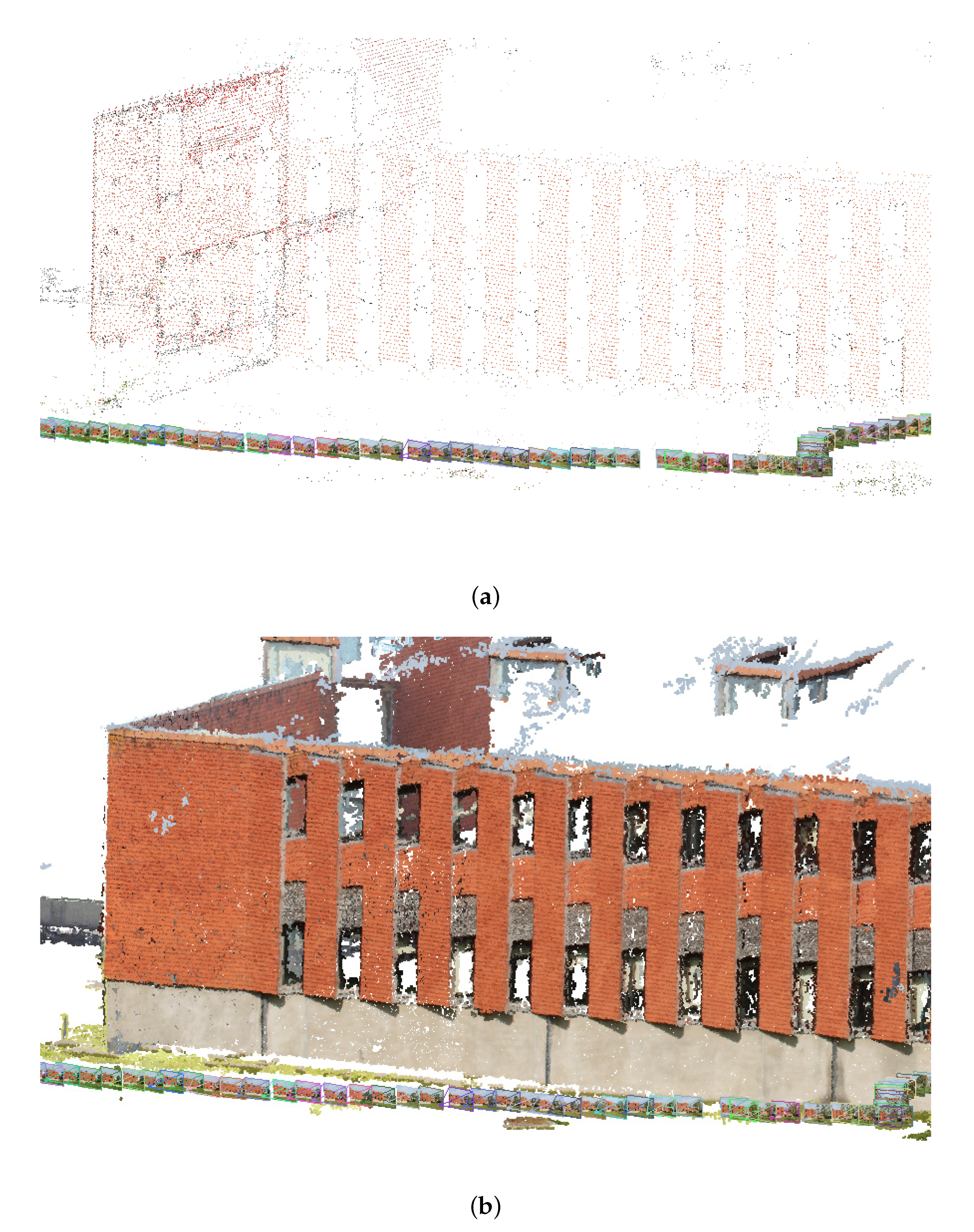
VisualSFM uses VLFeat [14] by default, a variation on the original Lowe implementation of SIFT [15], which is available freely under the Berkeley Software Distribution (BSD) License [14]. An example of feature vectors generated by SIFT is shown in Figure 1. The set of features defined by SIFT can contain outliers or points not common to both images (depending on the overlap). VisualSFM quickly and robustly matches images by using the iterative technique RANdom SAmple Consensus (RANSAC) [16], which constructs an eight-point alignment model in linear time. Bundle adjustment refines a visual reconstruction to jointly produce the optimal 3D structure and the viewing parameters. An example of the final result after bundle adjustment is shown in Figure 2a. Although it is not essential to use the focal length to conduct bundle adjustment, using the exchangeable image file (EXIF) information to provide focal length information enables an initialization value that makes bundle adjustment much easier [17]; the approach that will be proposed herein adds the focal length to the video data. After bundle adjustment, VisualSFM uses multi-view stereo (CMVS) [18] to create a dense point cloud from the scene as, shown in Figure 2b.
A GoPro hero3+ silver [19] was used to obtain the footage for this study. The advantages of using a GoPro are that it is low-cost, extremely light, and robust. The hero3+ has the added advantage of supporting an ad hoc wireless network, which allows for images to be streamed directly to the user and enables the camera to be remotely controlled. Being able to view what the camera is seeing from the ground greatly accelerates data acquisition and reduces the number of flight repetitions required to obtain sufficient coverage.
The image size of the video footage is limited to 1080 by 1920 pixels due to the high frame rate and the size and sensitivity of the GoPro’s charge-coupled device (CCD). The phase alternating line (PAL) format [20] was used to capture footage at 25 frames per second. While higher resolution (2592 by 3872 pixels) is achievable through the still image mode, it can only be used to capture two frames per second and is, thus, incompatible with the remote operation controls. During initial investigations by the authors, such a low frame rate was also deemed insufficient to obtain the necessary overlap in unstabilized footage. Although this video footage has a lower resolution than still images, decreasing the image size does not necessarily degrade the performance of the SIFT Algorithm [21], because VisualSFM itself will re-size any image above 3200 pixels before processing [6].
Notably, the GoPro camera has a fixed wide angle lens, which causes significant distortion of the image on the CCD. VisualSFM will automatically correct for the radial distortion of a lens [22], but the program needs to adjust the fundamental matrix for the particular lens and camera system [23]. The necessary correction of lens distortion is discussed in more detail subsequently in this paper.
A QX350 quadcopter [3] was used as the UAV. This unit is stabilized using a combination of accelerometers and GPS information. The QX350 did not have a built-in camera, but instead came with a GoPro camera mount. The mount did not have axial stabilization, but was separated from the main body of the aircraft by four rubber connectors. The connectors prevented the vibrations from the motors affecting the video footage.
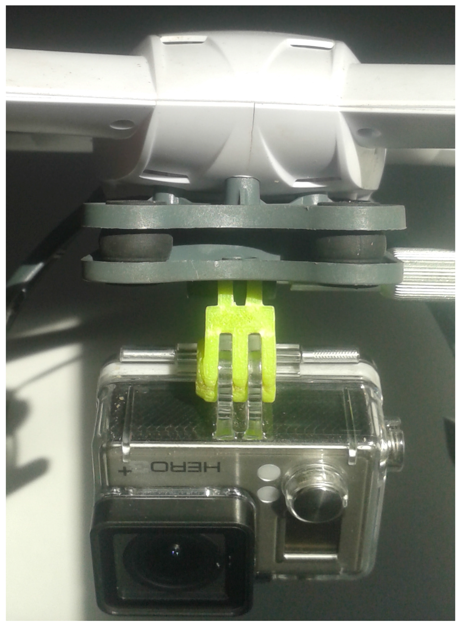
Initial investigations showed that the limited mounting angle (approximately 10° from the horizontal) unduly restricted the amount of ground capture in each image, which caused the SIFT algorithm to use many sky features as keypoints (see Figure 3). As these points are essentially “at infinity” and remain consistent for several images, the SIFT process generated artifacts (i.e., small groupings of points floating around the final model). To circumvent this problem, a small connector was designed and 3D printed for the camera mount, which allowed mounting the camera at a 45° angle (see Figure 4 for the equipment setup).
Although SFM is a fully-automatic methodology, several interventions are proposed as improvements. First, performance can be improved by reducing the number of variables that must be computed. Second, the radial distortion from the GoPro’s wide-angle lens can (and must) be corrected. Third, EXIF data (e.g., aperture settings for the focal number, focal length) are needed for the image processing but are not recorded in the video footage. Consequently, this must be introduced as a post-processing step.
The proposed solution involves taking a still image with the camera prior to obtaining the video footage and then adding the relevant EXIF information from that image to each subsequent video frame. The implementation developed to do this process automatically is available for download on Github [24]. The most important information for improving the quality of the reconstruction consists of the camera’s focal length and aperture. The camera make and model are added to find the fundamental matrix to correct for lens distortion.
VisualSFM is organized to compare every image in a set with every other one to find the best match. Although this approach is guaranteed to find the best match, it increases the time taken to complete the 3D reconstruction exponentially (). However, the sequential nature of video footage can be exploited by restricting the comparison within a pre-specified range of neighboring images. Thus, reconstruction time is reduced to a linear relationship, which allows for much larger datasets to be used in the reconstruction.
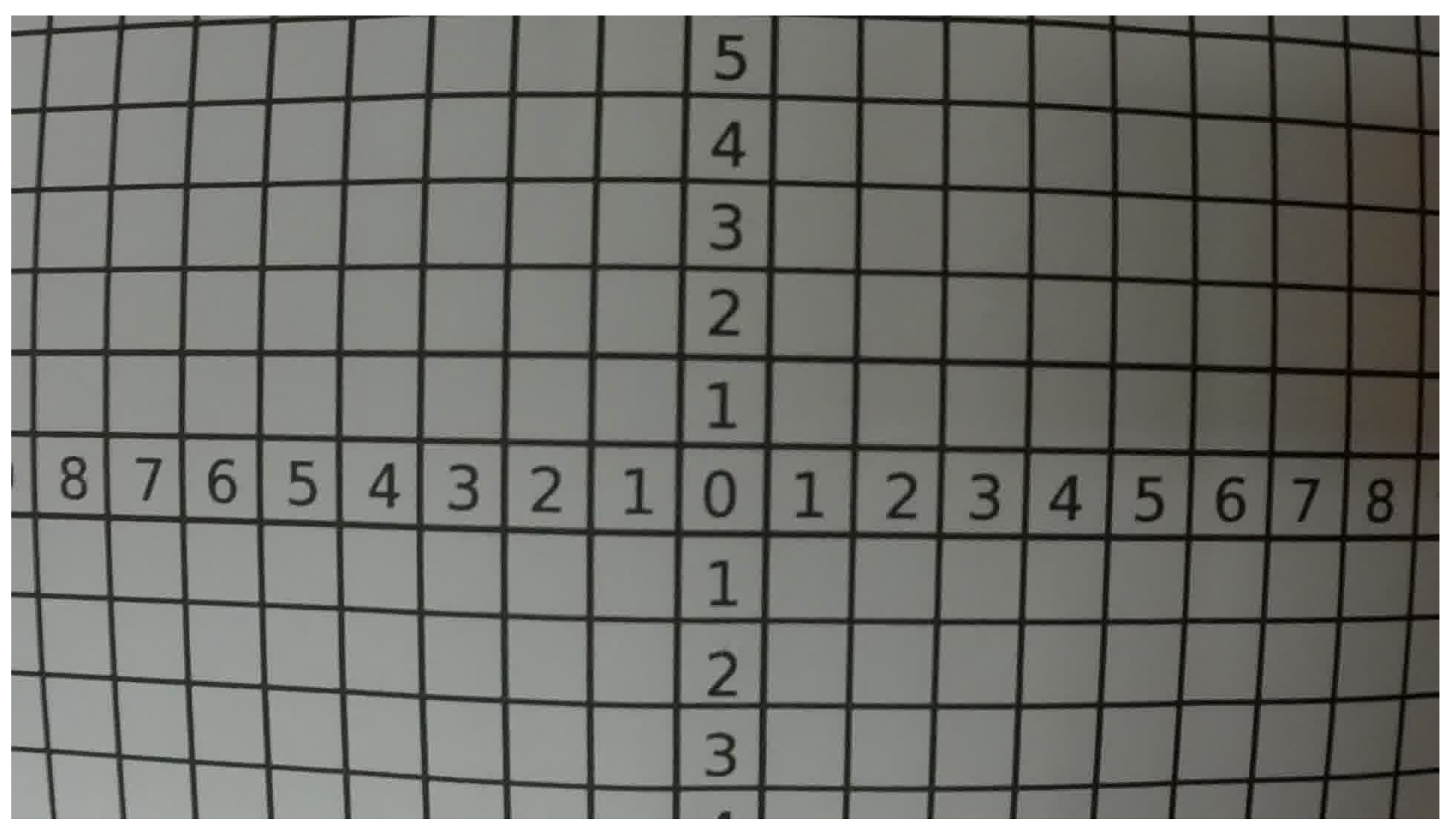
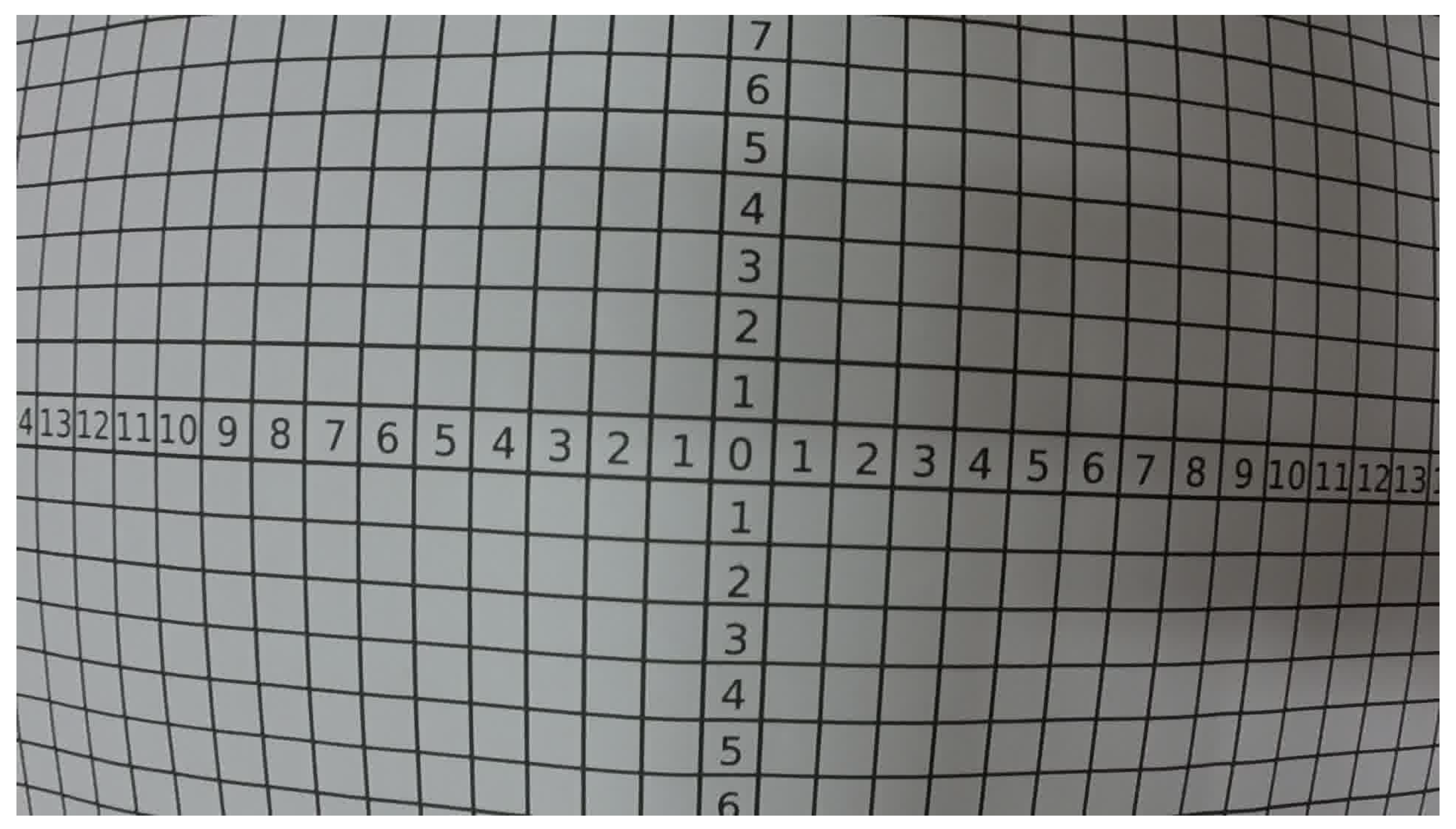
One variable that can have a large effect on the final result is the area captured, as shown in previous work [12]. One way to control this without altering distance is to change the FOV. The GoPro used in this experiment has three FOV settings: narrow, medium, and wide. The images for the video were fixed at 1080 by 1920 pixels for every FOV, while the coverage area and radial distortion varied. Figure 5, Figure 6 and Figure 7 show the differences in the distortion effects. The images were taken at a height of 15 cm, and each grid square was a centimeter wide. As video footage is always sampled at the same image size, there was a trade-off between the output quality (with the affiliated level of radial distortion) and the coverage area. To quantify this, each FOV experiment was designed to establish whether a less distorted, more detailed set of images generates a better 3D building reconstruction than a set containing more distorted images that cover a greater area.
The different FOVs generate imagery of the same quality, as they are all encoded at 1080p. Narrow FOV records video at 4 k then crops the images to 1080p. Medium FOV records video at 2.7 k then crops the images to 1080p. Wide FOV records at a 1080p resolution. One flight for each FOV setting was conducted to compare the settings. Each flight covered the same ground area and followed the same flight path. The distance from the camera to the building was 20 m, as this allowed for an entire side of the building to be captured in a single frame. The UAV was flown at a height of 10 m. The flights were not completely identical, as they were flown manually, and some turbulence was experienced, but they were of the same duration (3 min). The experiment was authorized by the University College Dublin (UCD) ethics committee (LS-E-14-59-Byrne-Laefer), and the obtained footage was anonymized by the SFM process.
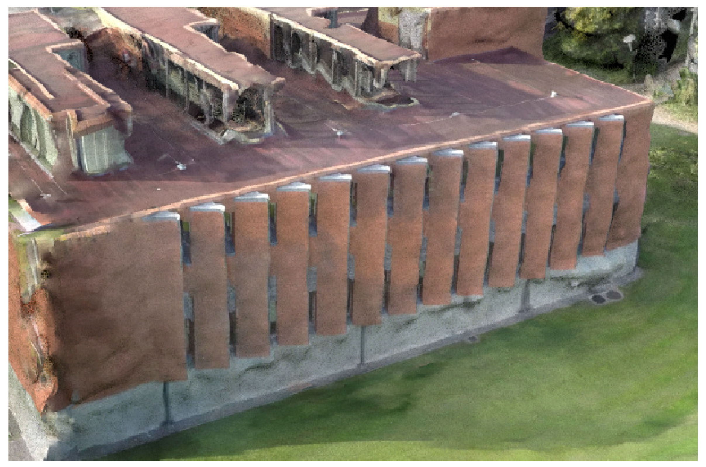
The target area chosen was the Urban Institute Ireland building on the UCD campus, as it had sufficient green space to allow for the quadcopter to be flown safely and away from any pedestrians. The building itself has an interesting design, and the east wall has a number of protrusions and surface features that facilitate comparisons between the output 3D models. The models were reconstructed and then compared with a terrestrial laser scanning (TLS)-based model obtained by a Leica ScanStation P20, a unit that claims millimeter-level precision, depending on the material [25]. The section of the east wall that was scanned for comparison resulted in a point cloud of 1,079,319 points and is shown in Figure 8.
The post-processing using VisualSFM was conducted on an Intel I7 3.4 GHz with 8 GB of RAM and an Nvidia GTX 770 graphics card. VisualSFM compared each image with 150 adjacent images in the sequence they were recorded (rather than the default 50) to find the best match. Previous tests showed that using these parameters enabled the processing of 4000 images in approximately 4 h.
To compare the VisualSFM outputs to the TLS-based model, the open-source software Cloudcompare [26], which uses an octree representation, was employed to find the nearest neighbor between the massive point cloud datasets. The distribution of the Euclidean distances was calculated and used to compare the accuracy of the FOV settings.
3. Results
A 3D reconstruction was generated for the three FOVs specified in Table 1. The details of the reconstruction are also shown in Table 1. The processing took approximately 4 h for each 3D reconstruction. Although the processing time is highly dependent on machine configuration, this example demonstrates the fundamental efficiency of VisualSFM to process large quantities of video data. Initial investigations showed that insufficient overlap between images resulted in a reconstruction mistakenly generating several separate models. In the actual experiment, each of the FOVs generated a single model, thereby indicating that video-based photogrammetry generates sufficient overlap to create coherent models.
The narrow FOV generated the most keypoints (85,274), and the CMVS reconstruction used those keypoints to generate a dense final point cloud of 1,338,408 points. The results showed that greater image resolution will allow more keypoints to be found, which enables a more detailed reconstruction. Although the narrowest FOV had the most keypoints and the densest point cloud reconstruction, the area covered (i.e., the surface area of the building captured in the reconstruction) was less than the other FOVs and captured only two of the three sides of the target building, as shown in Figure 9.
The medium FOV generated an almost identical number of keypoints to the narrow FOV (85,247) but resulted in a final point cloud of 1,326,065 points. While the medium FOV generated a similar number of keypoints to the narrow FOV, it covered a much greater area. The reconstruction picked up details on all sides of the building including the facades of the surrounding building, as shown in Figure 10.
Finally, the wide FOV only generated 42,942 keypoints, approximately 50% of the keypoints generated by the narrow FOV. This impacted the dense reconstruction, as shown by the resulting point cloud of only 622,055 points. The area covered by the wide FOV was comparable to the medium FOV, in which both of the buildings and surrounding facades were captured, as shown in Figure 11.
To compare the precision of the models and examine if there were artifacts stemming from radial distortion in the lens, the results were compared with TLS data collected from a laser scan of the east wall of the target building. For each point in the TLS reference model, the closest point in the FOV model was found, and the Euclidean was distance computed. The results for the Euclidean point comparison are shown in Table 2. There is an increase in distance around the edges of the facade for all of the FOVs, which could be a result of radial distortion from the lens.
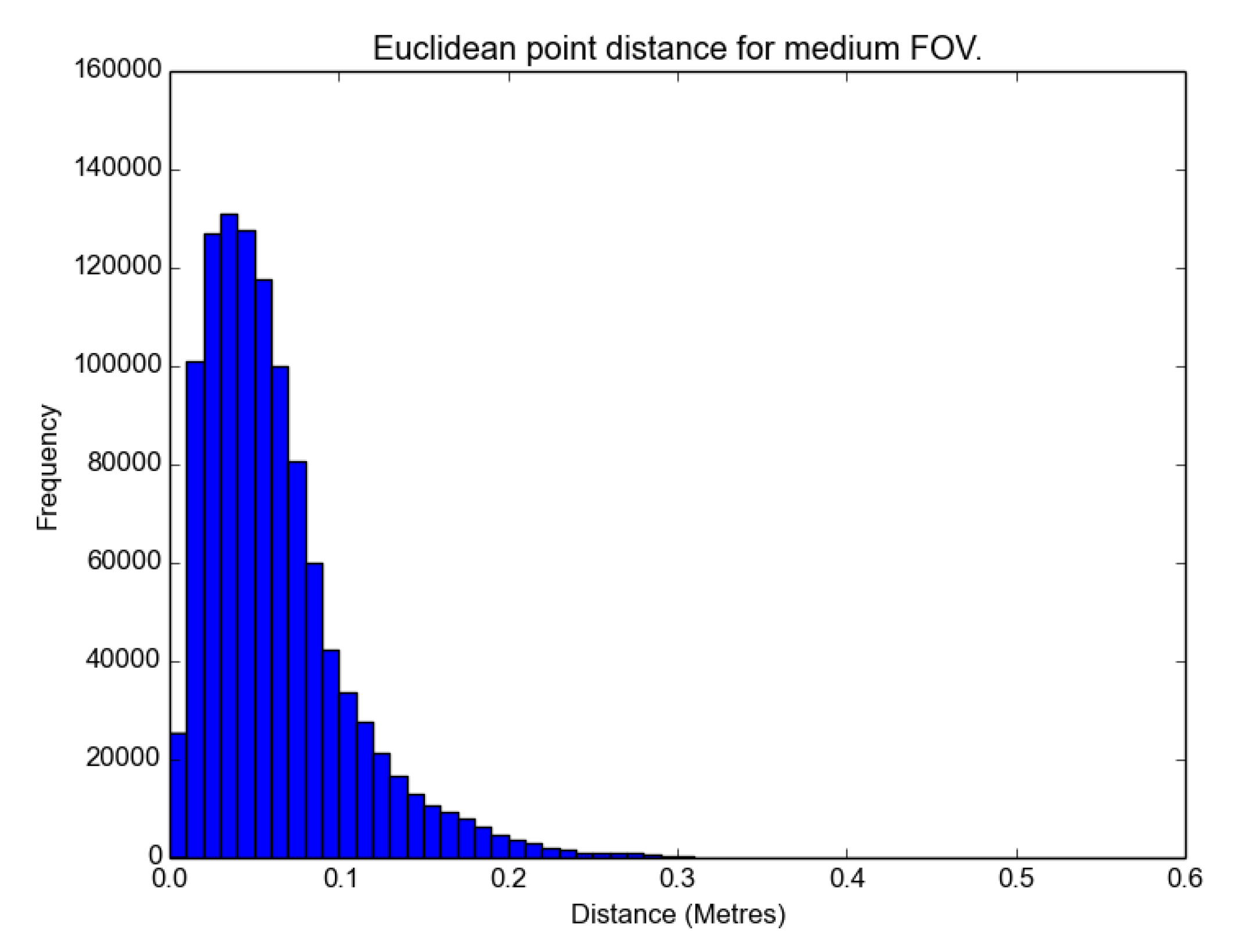
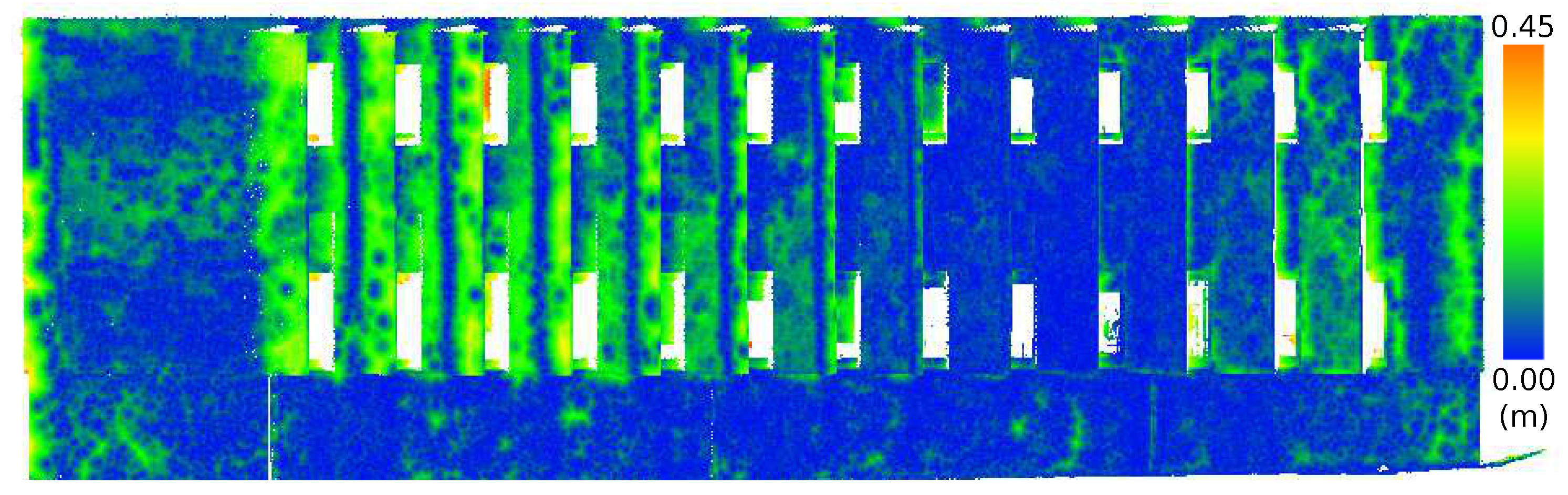
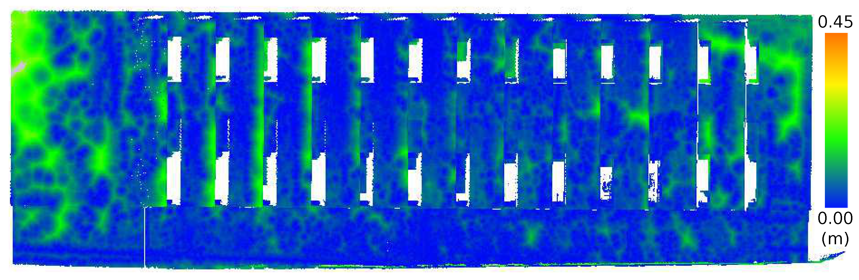
The distributions are not parametric, as there is a visible skew in the histograms in Figure 12, Figure 13 and Figure 14. The skew is caused by the Euclidean distance returning an absolute value. Such a bias will affect the interpretation of the mean and standard deviation, but as they all exhibit similar skew, some measure of relative comparison is possible. A Wilcoxon rank sum non-parametric test was performed on the distributions, and the results were shown to be statistically significant. The significance level of the Wilcoxon rank sum was 0.05. Whereas the histogram is the numerical indicator of error, the locations of the errors are indicated in Figure 15, Figure 16 and Figure 17. In these figures, the Euclidean distance for each point is shown where a small difference in distance is shown in blue, and a large difference in distance is highlighted in green and red. The colors automatically scale to the range of the histogram.
The results show that the medium FOV performed the best, as it has the lowest average error and standard deviation when compared to the LIDAR scan. This was followed closely by the wide FOV and finally the narrow FOV. Notably, the average error was less than 10 cm, and most surprisingly, there were not any significant effects of radial distortion from the lens in the images on the resulting models when comparing the FOV models with the TLS data, as shown in Figure 15, Figure 16 and Figure 17. The lack of radial distortion artifacts shows that the corrections to the fundamental matrix computed by VisualSFM succeeded in overcoming distortion generated by the low-cost, wide-angle lens.
4. Discussion
The experiments demonstrate competing priorities of capturing scene details and coverage. The narrow FOV generated the greatest number of points, but covered the smallest area, while the wide FOV covered a greater area, but generated a point cloud only half the size. The medium field of view successfully balanced these two constraints to generate the best model. The results also showed that the default VisualSFM correction for the radial distortion of the lens generated an accurate model.
While there was a difference in the models generated by the various FOVs, each created an impressive final result for only three minutes of flight and four hours of automatic processing. In contrast, a TLS scan of a building from several different viewpoints takes several hours of manual work both in obtaining the data and manually registering the point clouds afterwards.
Although the focus of this work was to compare the SFM generated point clouds, the images obtained during flight can be mapped onto the reconstructed model with additional post-processing steps. The point clouds are of sufficient quality that they can be meshed. Additionally, the bundle registers the camera location for each image. Thus, combining the mesh with the registered images enables a texture to be generated. The texture is then mapped back onto the mesh by using a software package such as Meshlab [27]. The results of this process are shown in Figure 18. Combining the reconstruction data with the original 2D image data generates a detailed 3D record of the surfaces of a structure. Such a record is useful for conservation and restoration work [28].
This work focused on a comparison of FOV settings and its effect on reconstruction. Future work in this area will include a comparison of different software such as the OpenMVG reconstruction pipeline and the use of different lens configurations to improve reconstruction quality.
5. Conclusions
This works demonstrates the ability to reconstruct high quality 3D models from noisy data obtained from a low-cost UAV by using video footage. Video footage provides a massive amount of data and at such a high frequency that it can minimize the effects of sudden camera movement. The addition of EXIF metadata to the images enables SFM to reconstruct a coherent 3D model from unstabilized data. This paper also investigated how changes in the field of view affected the reconstruction and showed that a medium field of view gives a balance of coverage and detail that generates the most accurate reconstruction. In addition to using video footage, this work shows that selecting the optimal FOV is important for striking a balance between sufficient detail for a dense reconstruction and adequate overlap to register a single model.
Acknowledgments
This work was generously supported by the European Union through Grant FP7-632227, IRC Grant GOIPD/2015/125, IRC Grant GOIPG/2015/3003, Geological Survey of Ireland Grant 2015-sc-Laefer and by Science Foundation Ireland Grant 13/TIDA/I274. Additional thanks to Andrea McMahon for her help and the DJEI/DES/SFI/HEAIrish Centre for High-End Computing (ICHEC) for the provision of computational facilities and support.
Author Contributions
Jonathan Byrne and Evan O’Keeffe conceived of and designed the experiments. Jonathan Byrne and Donal Lennon performed the experiments. Jonathan Byrne and Debra Laefer analyzed the data. Jonathan Byrne and Debra Laefer wrote the paper
Conflicts of Interest
The authors declare no conflict of interest.
References
- Markets and Markets. Unmanned Aerial Vehicle (UAV) Market (2013–2018); Markets and Markets: Seattle, WA, USA, 2013. [Google Scholar]
- Chen, S.; Laefer, D.F.; Mangina, E. State of technology review of civilian UAVs. Recent Pat. Eng. 2016, 10, 160–174. [Google Scholar] [CrossRef]
- Blade Helicopters. 350QX. Available online: http://www.bladehelis.com/350qx/ (accessed on 5 December 2016).
- Agisoft. Agisoft PhotoScan User Manual, Professional Edition, Version 1.0.0. Available online: http://downloads.agisoft.ru/pdf/photoscan-pro_1_0_0_en.pdf (accessed on 7 December 2016).
- Moisan, L.; Moulon, P.; Monasse, P. Automatic homographic registration of a pair of images, with a contrario elimination of outliers. Im. Proc. Line 2012, 2, 56–73. [Google Scholar] [CrossRef]
- Wu, C. VisualSFM: A Visual Structure from Motion System. Available online: http://ccwu.me/vsfm/ (accessed on 6 December 2016).
- Lucieer, A.; de Jong, S.M.; Turner, D. Mapping landslide displacements using Structure from Motion (SfM) and image correlation of multi-temporal UAV photography. Prog. Phys. Geog. 2014, 38, 97–116. [Google Scholar] [CrossRef]
- Mohanarajah, G.; Usenk, V.; Singh, M.; D’Andrea, R.; Waibel, M. Cloud-based collaborative 3D mapping in real-time with low-cost robots. IEEE Trans. Autom. Sci. Eng. 2015, 12, 423–431. [Google Scholar] [CrossRef]
- Gross, J.N.; Yu, G.; Rhudy, M.B. Robust UAV relative navigation with DGPS, INS, and peer-to-peer radio ranging. IEEE Trans. Autom. Sci. Eng. 2015, 12, 935–944. [Google Scholar] [CrossRef]
- Bailey, T.; Durrant-Whyte, H. Simultaneous localization and mapping (SLAM): Part II. IEEE Robot. Autom. Mag. 2006, 13, 108–117. [Google Scholar] [CrossRef]
- Fraser, C. Automated vision metrology: A mature technology for industrial inspection and engineering surveys. Aust. Surv. 2001, 46, 5–11. [Google Scholar] [CrossRef]
- Daftry, S.; Hoppe, C.; Bischof, H. Building with drones: Accurate 3d facade reconstruction using mavs. In Proceedings of the 2015 IEEE International Conference on Robotics and Automation, Seattle, WA, USA, 26–30 May 2015; pp. 3487–3494. [Google Scholar]
- Triggs, B.; McLauchlan, P.F.; Hartley, R.I.; Fitzgibbon, A.W. Bundle adjustment: A modern synthesis. In Vision Algorithms: Theory and Practice; Triggs, B., Zisserman, A., Szeliski, R., Eds.; Springer: Heidelberg, Germany, 1999; pp. 298–372. [Google Scholar]
- Vedaldi, A.; Fulkerson, B. VLFeat: An Open and Portable Library of Computer Vision Algorithms. Available online: http://www.vlfeat.org/ (accessed on 1 December 2016).
- Lowe, D.G. Object recognition from local scale-invariant features. In Proceedings of the Seventh IEEE International Conference on Computer Vision, Kerkyra, Greece, 20–27 September 1999; Volume 2, pp. 1362–1376. [Google Scholar]
- Fischler, M.A.; Bolles, R.C. Random sample consensus: a paradigm for model fitting with applications to image analysis and automated cartography. Commun. ACM 1981, 24, 381–395. [Google Scholar] [CrossRef]
- Snavely, N.; Seitz, S.M.; Szeliski, R. Photo tourism: exploring photo collections in 3D. ACM Trans. Graph. 2006, 25, 835–846. [Google Scholar] [CrossRef]
- Furukawa, T.; Ponce, J. Accurate, dense, and robust multiview stereopsis. IEEE Trans. Pattern Anal. Mach. Intell. 2010, 32, 1362–1376. [Google Scholar] [CrossRef] [PubMed]
- Woodman, N. GoPro Hero 3+. Available online: http://www.gopro.com/ (accessed on 25 November 2016).
- The ITU Radiocommunication Assembly. Recommendation ITU-R BT.470-6 Conventional Television Systems; International Telecommunication Union: Geneva, Switzerland, 1998; Available online: https://www.itu.int/ rec/R-REC-BT.470-6-199811-S/en (accessed on 1 December 2016).
- Hua, S.; Chen, G.; Wei, H.; Jian, Q. Similarity measure for image resizing using SIFT feature. EURASIP J. Image Video Proc. 2012, 2011, 1–11. [Google Scholar] [CrossRef]
- Wu, C. Critical configurations for radial distortion self-calibration. In Proceedings of the IEEE Conference on Computer Vision and Pattern Recognition, Columbus, OH, USA, 23–28 June 2014; pp. 25–32. [Google Scholar]
- Barreto, J.P.; Daniilidis, K. Fundamental matrix for cameras with radial distortion. In Proceedings of the Tenth IEEE International Conference on Computer Vision, Washington, DC, USA, 17–21 October 2005; pp. 625–632. [Google Scholar]
- O’Keeffe, E. Video Extractor, Adding EXIF Data to Video. Available online: https://github.com/eokeeffe/ videoExtractor (accessed on 3 December 2016).
- Leica Geosystems. Leica ScanStation P20 Industry’s Best Performing Ultra-High Speed Scanner. Leica Geosystems: Heerbrugg, Switzerland, 2013. Available online: http://w3.leica-geosystems.com/ downloads123/hds/hds/ScanStation_P20/brochures-datasheet/Leica_ScanStation_P20_DAT_en.pdf (accessed on 25 November 2016).
- Montaut, D.G. CloudCompare (Version 2.6) [GPL Software]. Available online: http://www.cloudcompare.org/ (accessed on 6 December 2016).
- Cignoni, P.; Callieri, M.; Corsini, M.; Dellepiane, M.; Ganovelli, F.; Ranzuglia, G. Meshlab: An open-source mesh processing tool. In Proceedings of the Sixth Eurographics Italian Chapter Conference, Salerno, Italy, 2–4 July 2008; pp. 129–136. Available online: http://vcg.isti.cnr.it/Publications/2008/CCCDGR08/ (accessed on 12 December 2016).
- Arias, P.; Caamaño, J.C.; Lorenzo, H.; Armesto, J. 3D modeling and section properties of ancient irregular timber structures by means of digital photogrammetry. Comput. Aided Civil Infrastruct. Eng. 2007, 22, 597–611. [Google Scholar] [CrossRef]
Figure 1.
Visualization of the keypoints and feature vectors found by SIFT in an image.
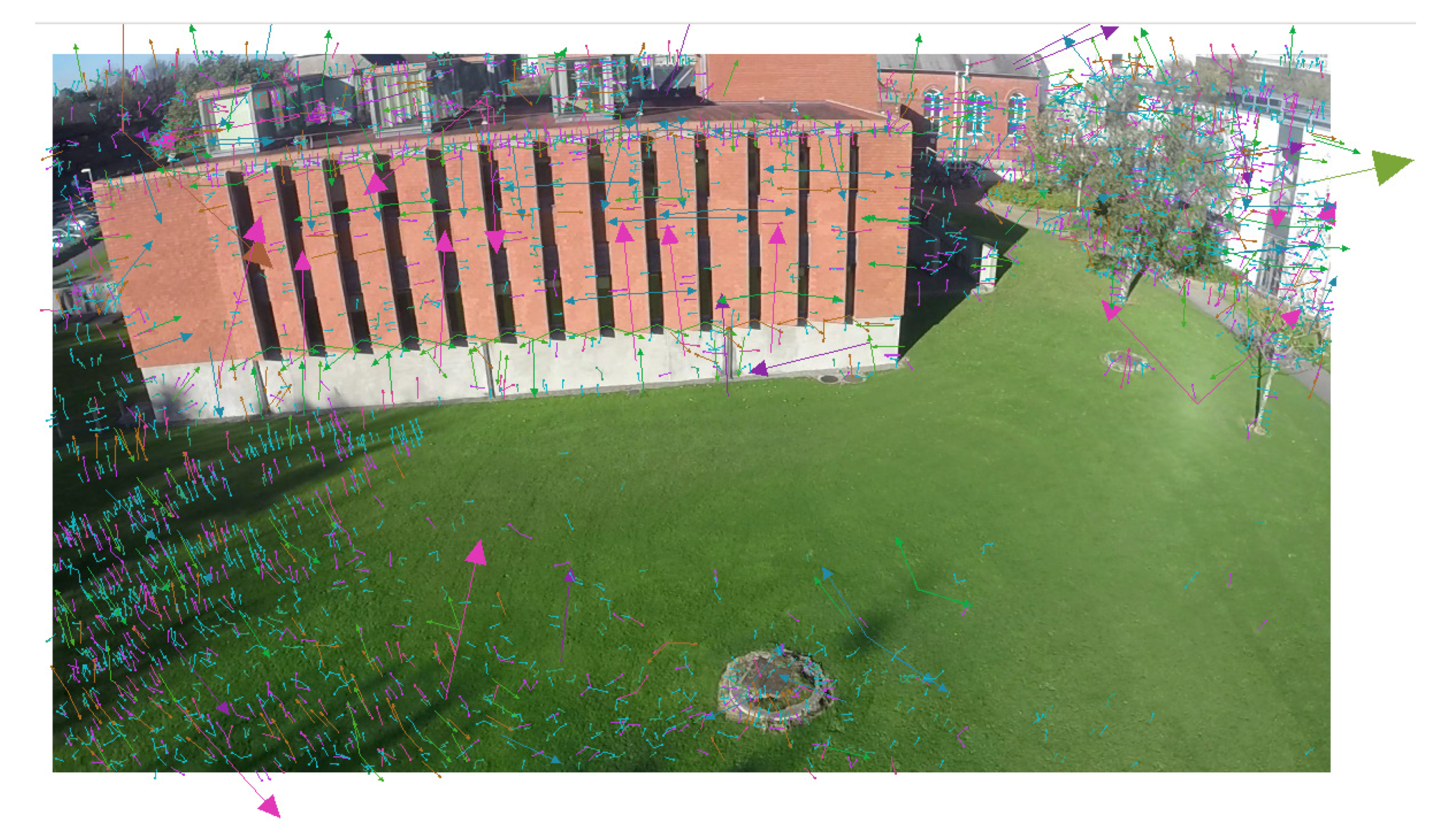
Figure 2.
A comparison of sparse and dense point clouds. (a) After bundle adjustment. The aligned camera frustums are on the bottom of the image, and the sparse reconstructed model from the SIFT keypoints are above. (b) Dense reconstruction of the image using multi-view stereopsis to fill the patches in the model.

Figure 3.
SIFT detecting spurious keypoints in the clouds.
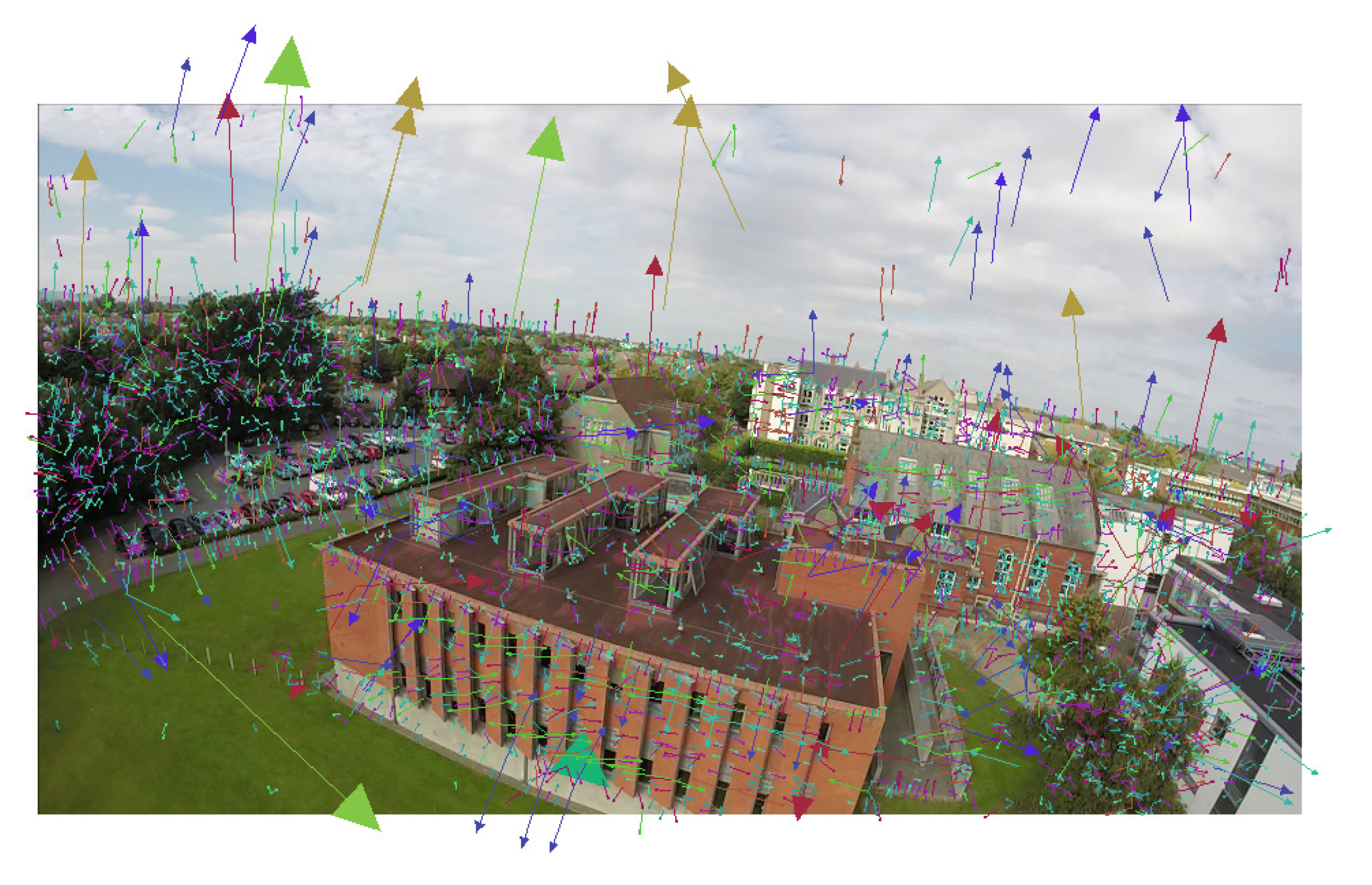
Figure 4.
GoPro attachment for the QX350. An additional connector was 3D printed to allow for a more oblique angle.
Figure 4.
GoPro attachment for the QX350. An additional connector was 3D printed to allow for a more oblique angle.

Figure 5.
Narrow field of view.

Figure 6.
Medium field of view.

Figure 7.
Wide field of view; note the increase in radial distortion.
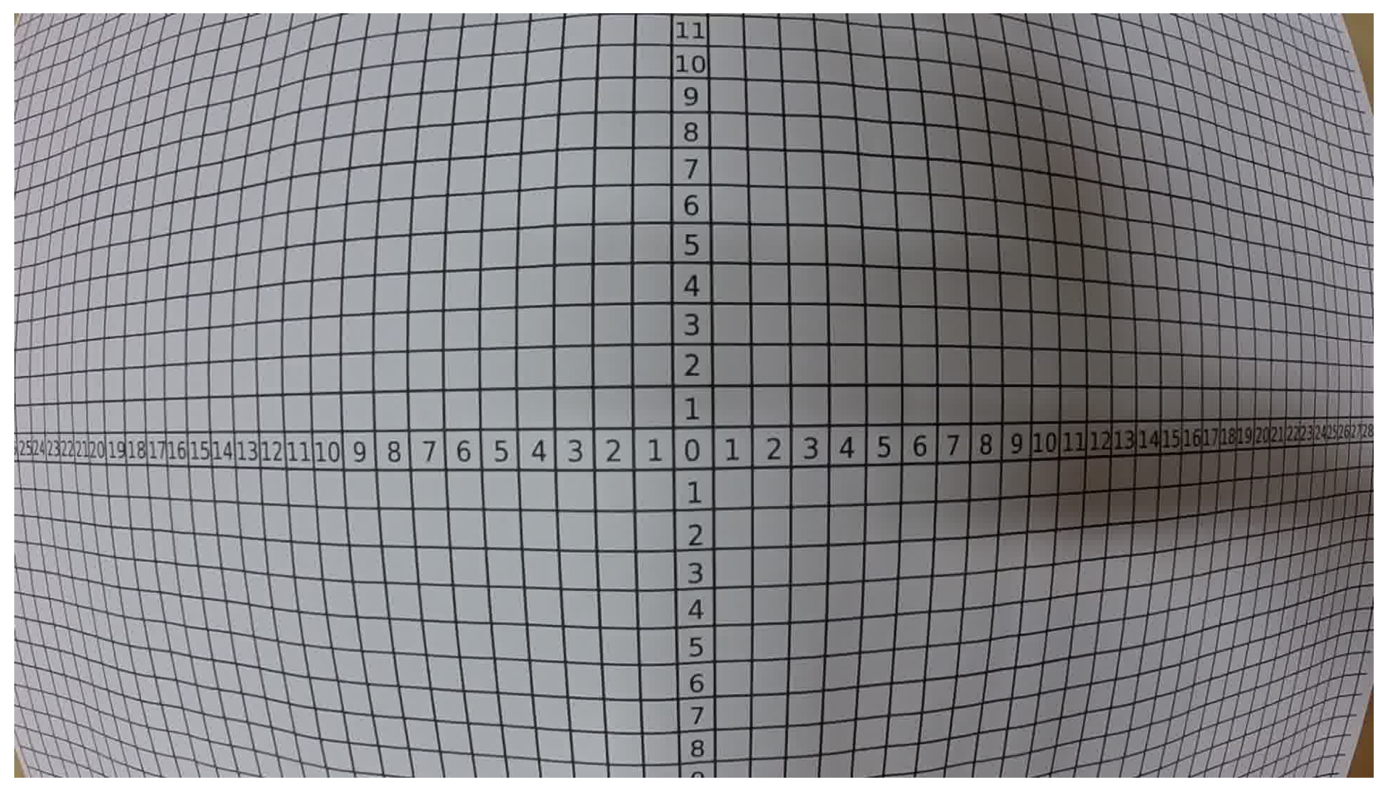
Figure 8.
Terrestrial laser scan of the east wall of the Urban Institute, Ireland.
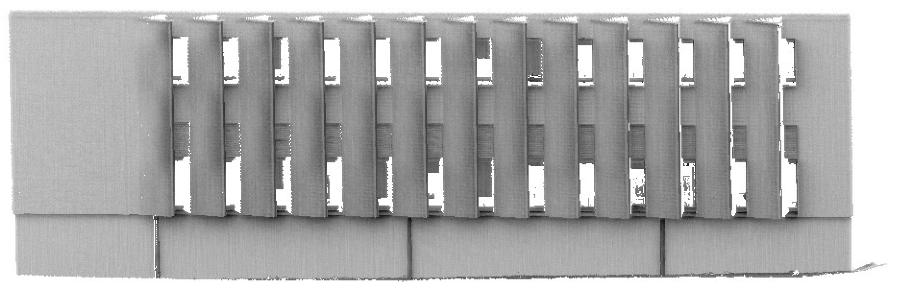
Figure 9.
Aerial view of the point cloud in natural RGB color generated by the narrow FOV. The black box highlights the area of the target building.
Figure 9.
Aerial view of the point cloud in natural RGB color generated by the narrow FOV. The black box highlights the area of the target building.
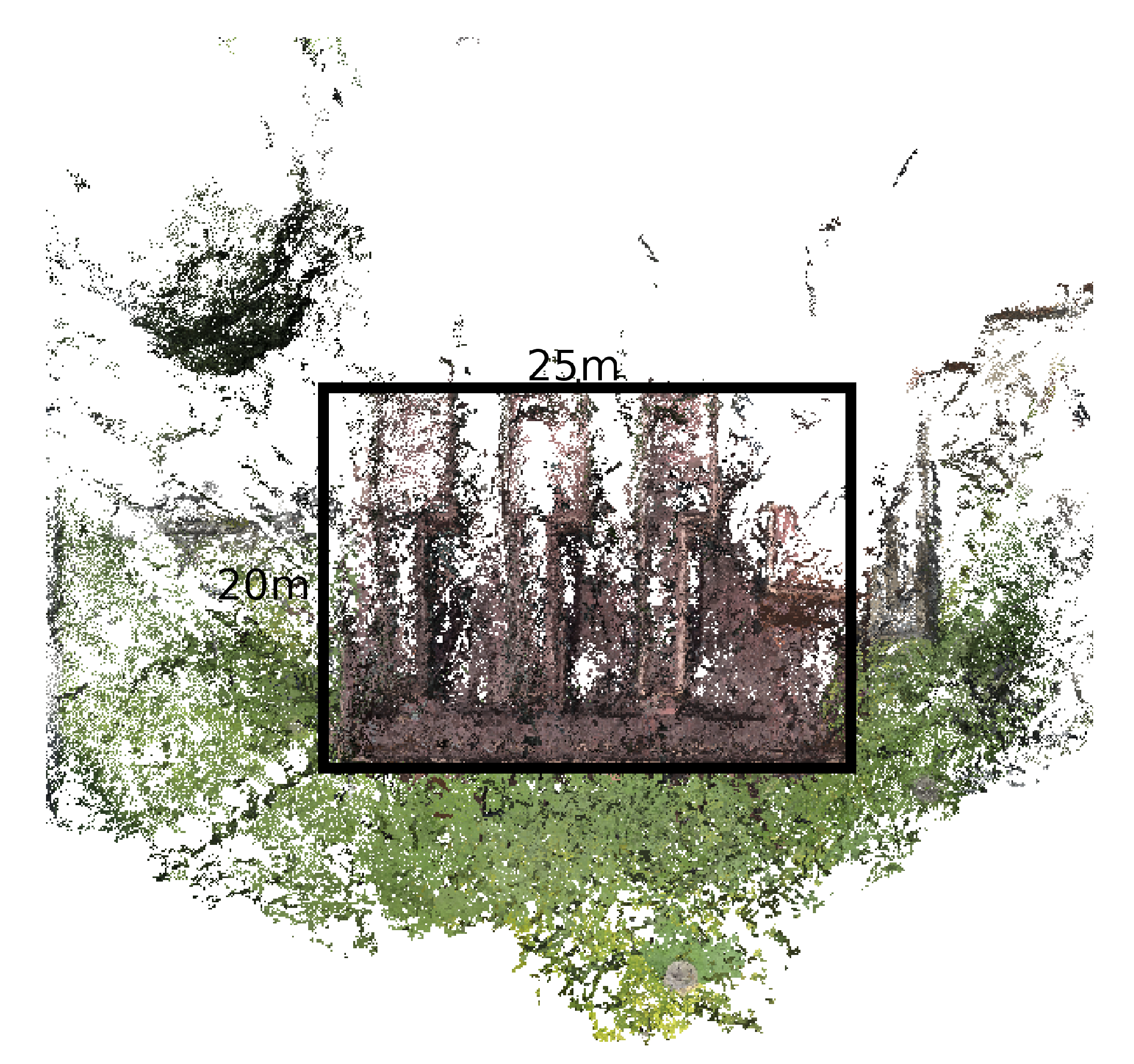
Figure 10.
Aerial view of the point cloud in natural RGB color generated by the medium FOV. The black box highlights the area of the target building.
Figure 10.
Aerial view of the point cloud in natural RGB color generated by the medium FOV. The black box highlights the area of the target building.
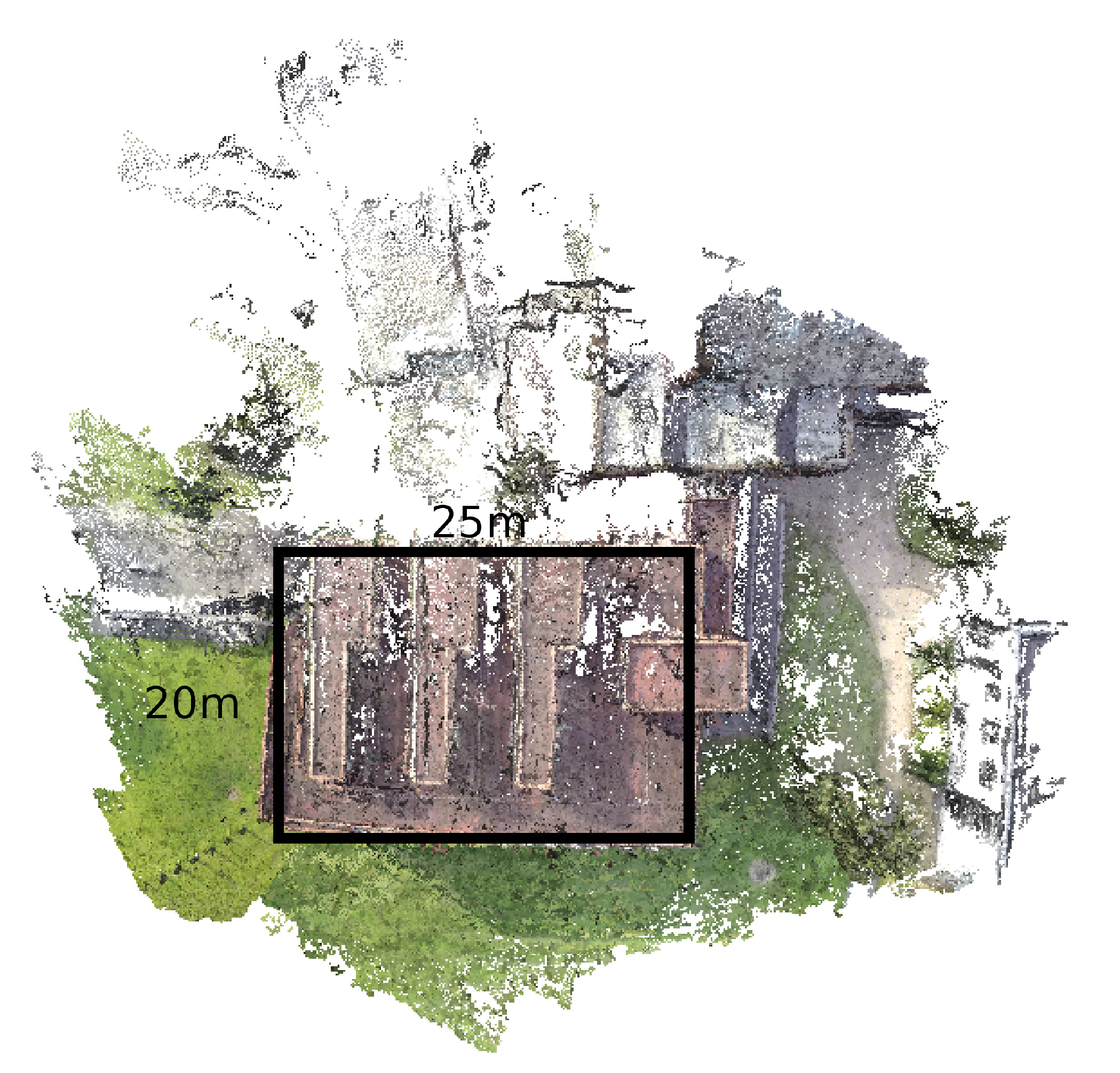
Figure 11.
Aerial view of the point cloud in natural RGB color generated by the wide FOV. The black box highlights the area of the target building.
Figure 11.
Aerial view of the point cloud in natural RGB color generated by the wide FOV. The black box highlights the area of the target building.
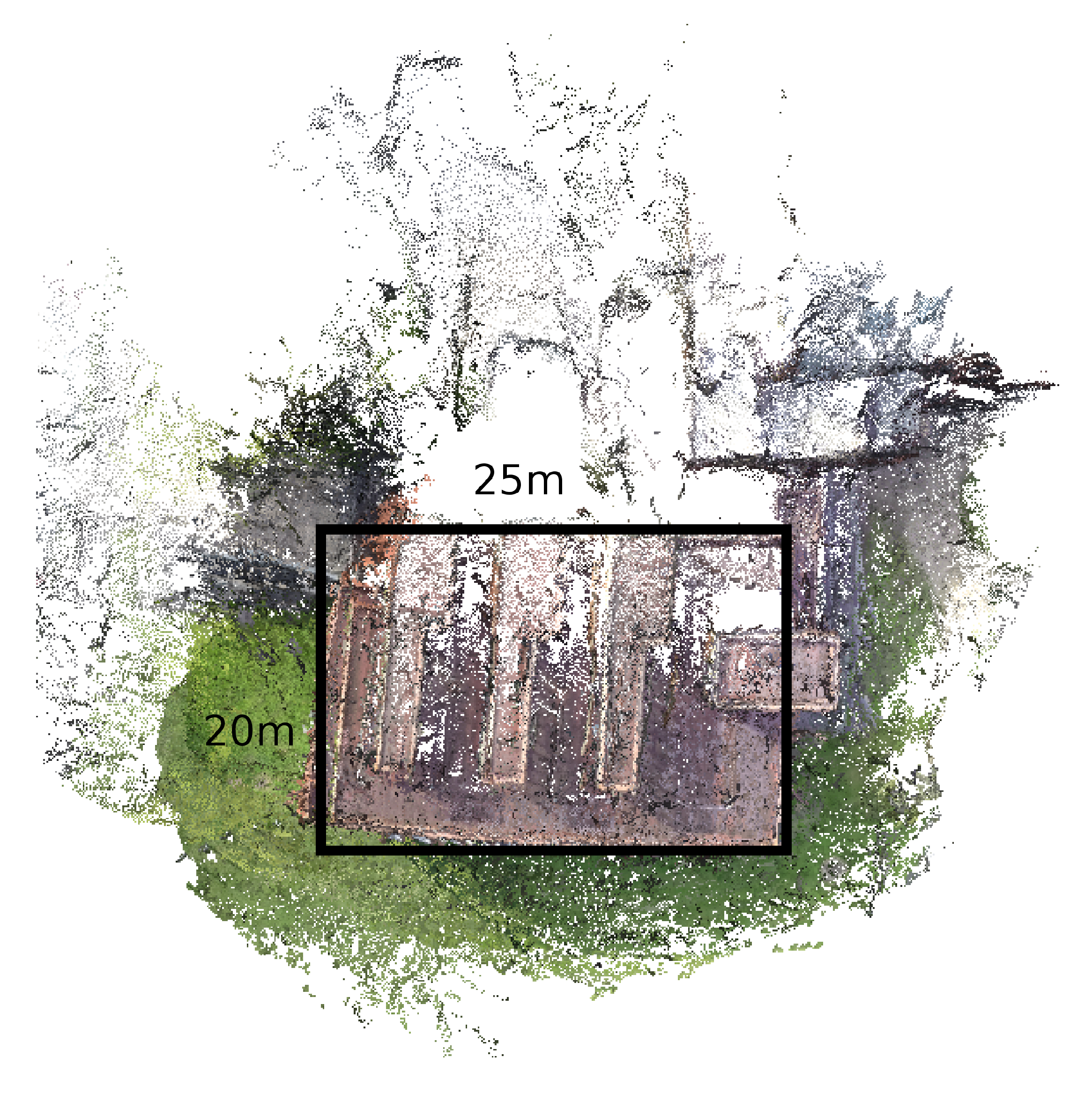
Figure 12.
Histogram of distances with a narrow field of view.
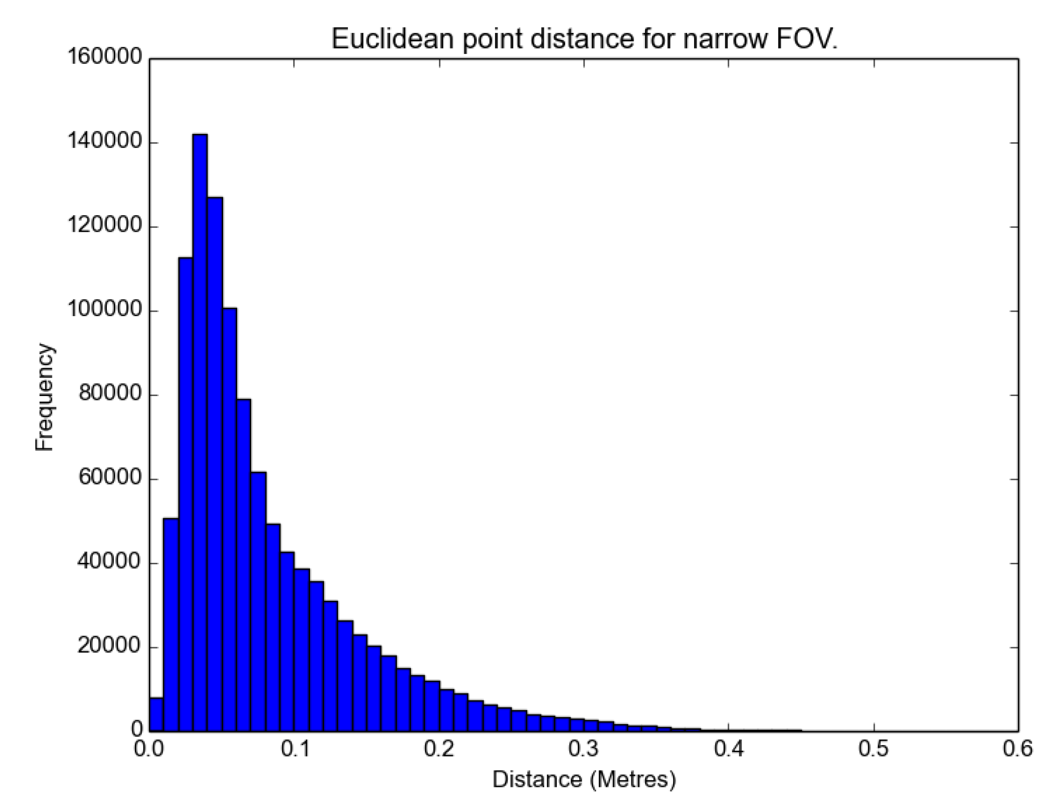
Figure 13.
Histogram of distances with a medium field of view.

Figure 14.
Histogram of distances with a wide field of view.
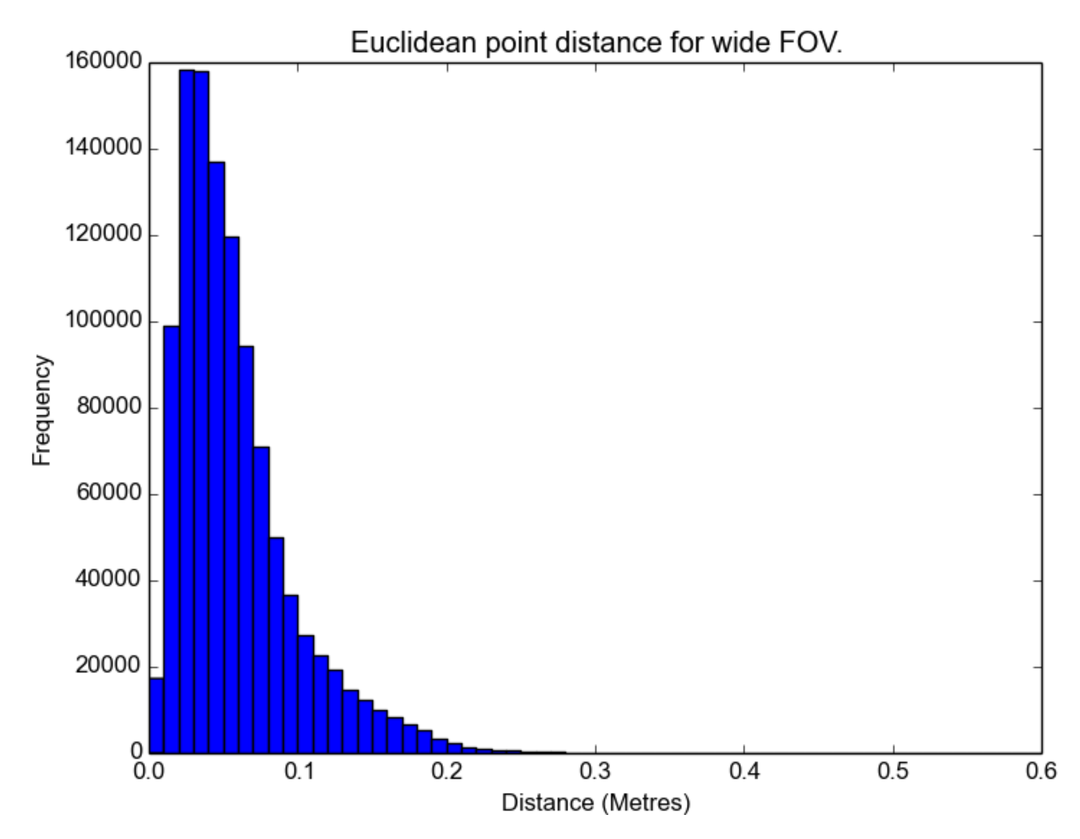
Figure 15.
Euclidean distances obtained from a narrow field of view (blue indicates a smaller Euclidean distance from the laser scan).
Figure 15.
Euclidean distances obtained from a narrow field of view (blue indicates a smaller Euclidean distance from the laser scan).

Figure 16.
Euclidean distances from using a medium field of view (blue indicates a smaller Euclidean distance from the laser scan).
Figure 16.
Euclidean distances from using a medium field of view (blue indicates a smaller Euclidean distance from the laser scan).

Figure 17.
Euclidean distances obtained from using a wide field of view (blue indicates a smaller Euclidean distance from the laser scan).
Figure 17.
Euclidean distances obtained from using a wide field of view (blue indicates a smaller Euclidean distance from the laser scan).
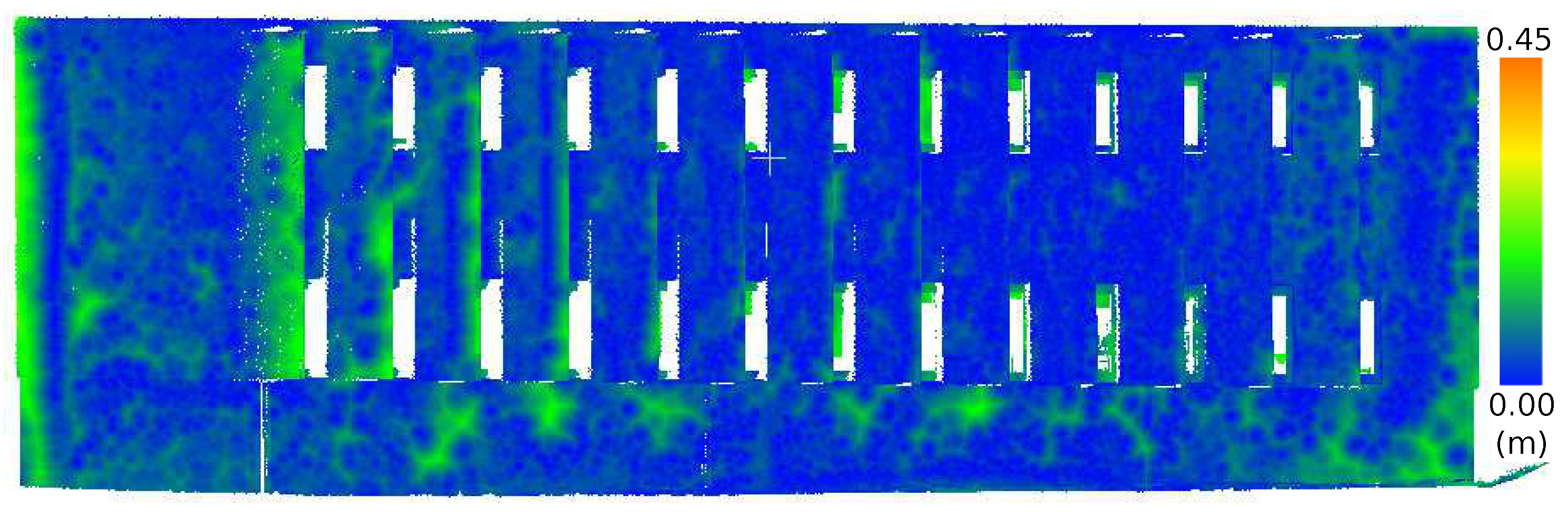
Figure 18.
The meshed model with texture from the captured images.

Table 1.
3D reconstruction processing information.
| Narrow FOV | Medium FOV | Wide FOV | |
|---|---|---|---|
| 49.1° × 64.6° × 79.7° | 72.2° × 94.4° × 115.7° | 94.4° × 122.6° × 149.2° | |
| No of Images | 3902 | 4048 | 4271 |
| Time Taken | 4 h 18 min | 4 h 6 min | 4 h 13 min |
| Models Generated | 1 | 1 | 1 |
| No. of Keypoints | 85,274 | 85,267 | 42,942 |
| No. of Points | 1,338,408 | 1,326,065 | 622,055 |
Table 2.
Comparative accuracy results for fields of view.
| Field of View | Min (m) | Max (m) | Average (m) | SD (m) |
|---|---|---|---|---|
| Narrow | 0.000559 | 0.5894 | 0.0826 | 0.066 |
| Medium | 0.000275 | 0.3501 | 0.0577 | 0.040 |
| Wide | 0.000483 | 0.4565 | 0.0621 | 0.043 |
© 2017 by the authors. Licensee MDPI, Basel, Switzerland. This article is an open access article distributed under the terms and conditions of the Creative Commons Attribution (CC BY) license (http://creativecommons.org/licenses/by/4.0/).
Share and Cite
MDPI and ACS Style
Byrne, J.; O'Keeffe, E.; Lennon, D.; Laefer, D.F. 3D Reconstructions Using Unstabilized Video Footage from an Unmanned Aerial Vehicle. J. Imaging 2017, 3, 15. https://doi.org/10.3390/jimaging3020015
AMA Style
Byrne J, O'Keeffe E, Lennon D, Laefer DF. 3D Reconstructions Using Unstabilized Video Footage from an Unmanned Aerial Vehicle. Journal of Imaging. 2017; 3(2):15. https://doi.org/10.3390/jimaging3020015
Chicago/Turabian StyleByrne, Jonathan, Evan O'Keeffe, Donal Lennon, and Debra F. Laefer. 2017. "3D Reconstructions Using Unstabilized Video Footage from an Unmanned Aerial Vehicle" Journal of Imaging 3, no. 2: 15. https://doi.org/10.3390/jimaging3020015
Note that from the first issue of 2016, this journal uses article numbers instead of page numbers. See further details here.