RGB Color Cube-Based Histogram Specification for Hue-Preserving Color Image Enhancement

Department of Communication Design Science, Kyushu University, Fukuoka 815-8540, Japan
*
Author to whom correspondence should be addressed.
J. Imaging 2017, 3(3), 24; https://doi.org/10.3390/jimaging3030024
Submission received: 1 June 2017
/
Revised: 27 June 2017
/
Accepted: 27 June 2017
/
Published: 1 July 2017
(This article belongs to the Special Issue Color Image Processing)
Abstract
:A large number of color image enhancement methods are based on the methods for grayscale image enhancement in which the main interest is contrast enhancement. However, since colors usually have three attributes, including hue, saturation and intensity of more than only one attribute of grayscale values, the naive application of the methods for grayscale images to color images often results in unsatisfactory consequences. Conventional hue-preserving color image enhancement methods utilize histogram equalization (HE) for enhancing the contrast. However, they cannot always enhance the saturation simultaneously. In this paper, we propose a histogram specification (HS) method for enhancing the saturation in hue-preserving color image enhancement. The proposed method computes the target histogram for HS on the basis of the geometry of RGB (rad, green and blue) color space, whose shape is a cube with a unit side length. Therefore, the proposed method includes no parameters to be set by users. Experimental results show that the proposed method achieves higher color saturation than recent parameter-free methods for hue-preserving color image enhancement. As a result, the proposed method can be used for an alternative method of HE in hue-preserving color image enhancement.
1. Introduction
Color image enhancement is a challenging task in digital image processing with broad applications including human perception, machine vision applications, image restoration, image analysis, image compression, image understanding and pattern recognition [1], underwater image enhancement and image enhancement of low light scenes [2]. Sharo and Raimond surveyed the existing color image enhancement methods such as histogram equalization (HE), fuzzy-based methods and other optimization techniques [3]. Saleem and Razak also surveyed color image enhancement techniques using spatial filtering [4]. Suganya et al. analyzed the performance of various enhancement techniques based on noise ratio, time delay and quality [5].
In color image enhancement, preserving the hue of an input image is frequently required to preserve the appearance of the objects in the image. Bisla surveyed hue-preserving color image enhancement techniques [6]. Zhang et al. proposed a method for hue-preserving and saturation scaling color image enhancement using optimal linear transform [7]. Aashima and Verma proposed a hue-preserving and gamut problem-free color image enhancement technique, and compared it with a discrete cosine transform-based method [8]. Porwal et al. also proposed an algorithm for hue-preserving and gamut problem-free color image enhancement [9]. Chien and Tseng proposed a set of formulae for the color transformation between RGB (red, green and blue) and exact HSI (hue, saturation and intensity), and used it for color image enhancement [10]. Gorai and Ghosh considered image enhancement as an optimization problem and solved it using particle swarm optimization [11]. Taguchi reviewed color systems and color image enhancement methods, and introduced an improved HSI color space [12]. Menotti et al. proposed two fast hue-preserving HE methods based on 1D and 2D histograms of RGB color space for color image contrast enhancement [13]. Pierre et al. [14] introduced a variational model for the enhancement of color images, and compared their method with the state-of-the-art methods including Nikolova and Steidl’s method [15], which is based on their strict ordering algorithm for exact HS [16].
Almost all of the above hue-preserving color image enhancement methods are based on the pioneering work of Naik and Murthy [17], where a scheme is proposed to avoid gamut problem arising during the process of enhancement of the intensity of color images using a general hue-preserving contrast enhancement function, in which HE is a typical example for intensity transformation. Han et al. also proposed the equivalent method from a viewpoint of 3D color HE [18]. However, Naik and Murthy’s method cannot increase the saturation of colors to be enhanced. To overcome this problem, Yang and Lee [19] proposed a modified hue-preserving gamut mapping method that outputs higher saturation than Naik and Murthy’s method. Yang and Lee’s method divides the range of luminance into three parts corresponding to dark, middle and bright colors, and handles the input colors in different manners, that is, for dark and bright colors, their saturation is enhanced first, and then, Naik and Murthy’s method is applied to the saturation-enhanced colors. On the other hand, for the remaining colors with middle luminance, Naik and Murthy’s method is applied to the original colors directly. Therefore, the saturation of the middle luminance colors cannot be improved as well as Naik and Murthy’s method.
In this paper, we propose a parameter-free HS method for hue-preserving color image enhancement based on the geometry of RGB color space. The proposed method can improve the color saturation in both Naik and Murthy’s and Yang and Lee’s methods. Experimental results show that the proposed HS method applied to Naik and Murthy’s and Yang and Lee’s methods improves the color saturation compared with the conventional Naik and Murthy’s and Yang and Lee’s methods using HE.
The rest of this paper is organized as follows: Section 2 first defines the saturation of a color, and then summarizes Naik and Murthy’s and Yang and Lee’s methods. Section 3 describes the detailed procedures of HS for color image enhancement, where HE is also summarized, and then RGB color cube-based HS method is proposed. Section 4 shows experimental results of hue-preserving color image enhancement. Finally, Section 5 discusses the results and the utility of the proposed method.
2. Hue-Preserving Color Image Enhancement
In this section, we briefly summarize previous hue-preserving color image enhancement methods proposed by Naik and Murthy [17] and Yang and Lee [19] after the description of color saturation.
Let be a point in RGB color space or an RGB color vector, where and b denote red, green and blue values, respectively, and satisfy and , and the superscript T denotes the matrix transpose. Then, the intensity of is given by [17] satisfying , and the saturation of is the perpendicular distance from the intensity axis to [20] as follows:
where , I is the identity matrix, and denotes the Euclidean norm.
Lemma 1.
The saturation of given by (1) has the following properties:
where β is a positive number, and
for .
The proof of Lemma 1 is given in Appendix A.
2.1. Naik and Murthy’s Method
Let for , where is a function of l for transforming the original intensity into the modified one in the same range as its domain, i.e., . Then, Naik and Murthy considered a hue-preserving transformation of the form
where denotes the transformed color vector of . The value of will be greater than 1 when . In such a case, the element value of may exceed 1 and thus result in a gamut problem. To overcome this problem, Naik and Murthy proposed a gamut problem-free procedure as follows:
Naik and Murthy’s method
- Case (i) If , then compute .
- Case (ii) If , then perform the following procedure:
- (1)
- Transform the RGB color vector to CMY (cyan, magenta and yellow) color vector , where and .
- (2)
- Find .
- (3)
- Find . Note that since .
- (4)
- Compute .
- (5)
- Transform the CMY color vector to RGB color vector .
Note that, in Step (3) in Case (ii), we cannot compute when because it results in division by zero. To avoid such difficulties, we set that if , and if . We find that Case (ii) can be concisely written as follows:
Case (ii) If , then compute for .
Additionally, it has been proved that Naik and Murthy’s method does not increase the saturation, that is, [21].
2.2. Yang and Lee’s Method
Yang and Lee also pointed out that the color saturation of the resulting images by Naik and Murthy’s method is low, and proposed a hue-preserving gamut mapping method, the resulting images of which show higher saturation than that of Naik and Murthy’s.
Although Yang and Lee defined the luminance of as instead of the intensity l to describe algorithms in their paper [19], we would like to use l rather than n in this paper consistently. Using l, we can describe Yang and Lee’s method as follows:
Yang and Lee’s method
- Case (I) If , then compute , whose intensity is 1. Apply Naik and Murthy’s method to as follows:
- (1)
- Case (I-i) If , then compute .
- (2)
- Case (I-ii) If , then compute .
- Case (II) If , then apply Naik and Murthy’s method to as follows:
- (1)
- Case (II-i) If , then compute .
- (2)
- Case (II-ii) If , then compute .
- Case (III) If , then transform into the CMY color vector , and then lower the intensity of to 2 as to have the RGB color vector . Apply Naik and Murthy’s method to as follows:
- (1)
- Case (III-i) If , then compute .
- (2)
- Case (III-ii) If , then compute .
We have the following lemma:
Lemma 2.
The saturation given by Yang and Lee’s method is greater than or equal to that given by Naik and Murthy’s method, that is, .
The proof of Lemma 2 is given in Appendix A.
3. Histogram Specification for Color Image Enhancement
Let be a digital color image, where denotes the RGB color vector at the position of a pixel in P for and , where m and n denote the numbers of pixels in the vertical and horizontal directions in P, respectively. Suppose that P is a 24-bit true color image. Then, each element of is an integer between 0 and 255, i.e., , and the intensity of is given by , where .
3.1. Histogram Equalization
Let be the histogram of the intensity of in P. Then, the th element of is given by , where denotes the Kronecker delta; if and 0, otherwise. Let be the cumulative histogram of , where the th element of is given by . Then, the intensity transformation function for HE is given by
where ‘’ operator rounds a given argument toward the nearest integer, , and for . The histogram-equalized intensity image of P is given by where
3.2. Histogram Specification
Let be a target histogram into which we want to transform the original histogram of intensity, and let be the cumulative histogram of , where the th element of is given by . Then, the intensity transformation function for HS is given by
where , and for . The histogram-specified intensity image of P is given by where
3.3. RGB Color Cube-Based Histogram Specification
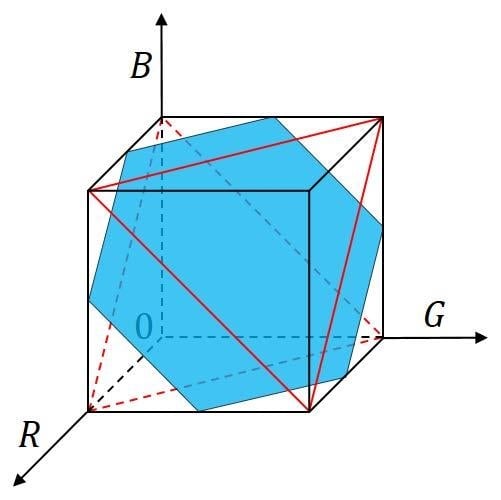
In this subsection, we propose a parameter-free HS method named RGB color-cube based HS. As described in Section 2, the saturation of a color in RGB color space is defined as the perpendicular distance between the intensity axis and a point corresponding to the color. The locus of the perpendicular line around the intensity axis forms an equiintensity plane. Let us consider the cross section of the equiintensity plane and RGB color cube as shown in Figure 1, where the cross sections are painted in light blue, and Figure 1a–c show three cases of the value of the intensity l found in the equation of the plane, , that is, and , respectively. In these figures, the triangles drawn by red broken and solid lines denote the cross sections of and , respectively.
The area of the cross section indicates the variety of saturation for a given intensity l. Let be the area of the cross section for an intensity l. Then, we have the following analytic form of :
which is continuous at and , that is, and . Additionally, the derivative function of is given by
which is also continuous at and , that is, and . The integral of is given by
which is also continuous at and , that is, and . Figure 2 shows the graphs of and , where the vertical and horizontal axes denote the function value of or and the intensity l, respectively, and the blue and green lines denote the functions and , respectively.
We propose to use and as the substitution of the target histogram and its cumulative one in HS, respectively. The detailed procedure is as follows.
Let be the target histogram for the proposed RGB color cube-based HS. Then, the th element of is given by
for . By means of the cumulation of , we have the cumulative histogram . In another way, since we have the analytic form of the integral of as , we can also compute from directly as follows:
for . Then, the intensity transformation function for RGB color cube-based HS is given by
where , and for . The histogram-specified intensity image of P is given by where
The above intensity transformation functions, and , can be used instead of in Naik and Murthy’s and Yang and Lee’s methods.
3.4. Conditions for Saturation Improvement
The above RGB color cube-based HS can be used in both Naik and Murthy’s and Yang and Lee’s methods as well as the conventional HE. In this subsection, we summarize the conditions for improving color saturation by the proposed HS compared with HE in the two methods.
3.4.1. Naik and Murthy’s Method
Let , and be the enhanced color of by Naik and Murthy’s method with the proposed HS. Then, we have under the following conditions:
3.4.2. Yang and Lee’s Method
Let be the enhanced color of by Yang and Lee’s method with the proposed HS. Then, we have under the following conditions for three cases of l:
If (Case I in Yang and Lee’s method), then we have the following conditions:
If (Case II in Yang and Lee’s method), then we have the same conditions as Equation (16) because Yang and Lee’s method coincides with Naik and Murthy’s method.
If (Case III in Yang and Lee’s method), then we have the following conditions:
4. Experimental Results
In this section, we show the experimental results of hue-preserving color image enhancement, and demonstrate that the proposed method improve the color saturation in comparison with Naik and Murthy’s and Yang and Lee’s methods using HE.
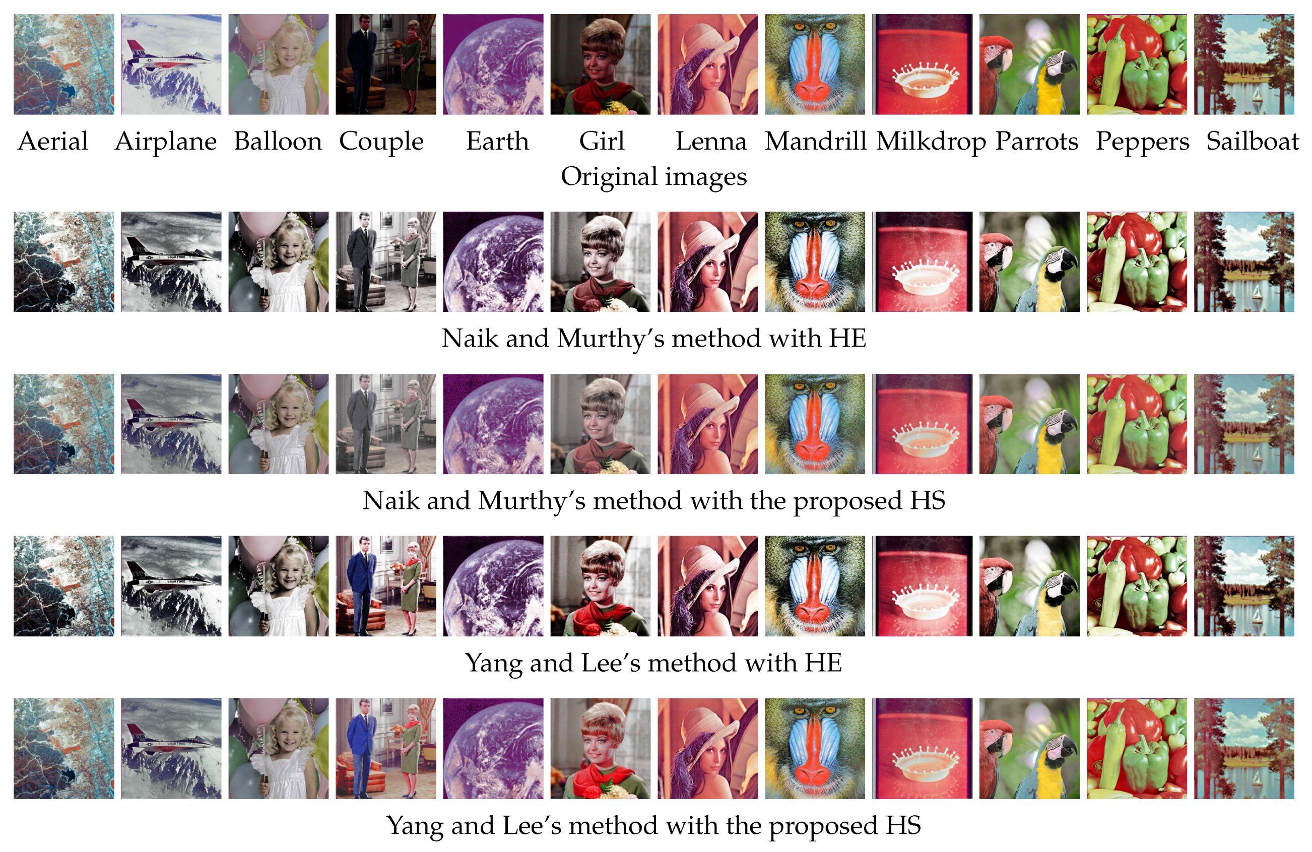
Figure 3 shows input and output images for hue-preserving color image enhancement, where the first top row shows the original input images, and the second to fifth rows show the corresponding output images. The original images in the top row are collected from the Standard Image Data-BAse (SIDBA) [22]. The second row shows the results by Naik and Murthy’s method, which uses HE for intensity transformation to enhance the contrast. However, the color saturation has faded in all images. As a result, the output images become close to their contrast-enhanced grayscale images. Moreover, we can see that the 2nd (Airplane) and the 6th (Girl) images become noisy by contrast overenhancement caused by HE. The third row shows the results of the proposed HS used in Naik and Murthy’s method instead of HE, where the color saturation is recovered and the noise is suppressed compared with the second row. The fourth row shows the results of Yang and Lee’s method with HE, where the 4th (Couple) and 6th (Girl) images have improved saturation and are more colorful than the second row of Naik and Murthy’s method. However, the other images are similar to that of Naik and Murthy’s method. The fifth row shows the results of the proposed HS used in Yang and Lee’s method instead of HE, where the saturation is improved compared with the third and fourth rows.
Figure 4 shows the saturation images whose pixel values are given by the saturation values in Equation (1). The order of the images are the same as that of Figure 3. The images in the second row are not brighter than that in the first row, which demonstrates visually that Naik and Murthy’s method cannot increase the saturation from the original images. The third row shows the saturation images by Naik and Murthy’s method with the proposed HS, which can improve the saturation—for example, we can see brighter regions in 7th (Lenna) to 10th (Parrots) images than the corresponding images in the second row. The fourth row shows the saturation images by Yang and Lee’s method with HE, which achieves higher saturation than Naik and Murthy’s method in the second row. The fifth row shows the saturation images by Yang and Lee’s method with the proposed HS, which further increases the saturation compared with the fourth row.
Figure 5 shows the difference maps between the enhanced and original saturation images. These maps are generated by the following procedure: let and be the corresponding pixels of an original color image and its enhanced one, respectively. Then, we compute the difference of their saturations as , and set the pixel color in the difference map by if , and otherwise. That is, cyan and green in the difference map mean a decrease and increase in saturation, respectively, and gray means neutral.
The top row in Figure 5 shows the difference maps between Naik and Murthy’s results with HE and the original images, where we can see a number of deep cyan regions, which mean a decrease in saturation from the original images. On the other hand, the second row shows the results by Naik Murthy’s method with the proposed HS, where the cyan regions are diluted compared with the top row. The third row shows the results by Yang and Lee’s method with HE, which gives similar results to Naik and Murthy’s method in the top row except for the 4th (Couple) and 6th (Girl) images, in which we can see the yellow regions that mean the increase in saturation. The bottom row shows the results by Yang and Lee’s method with the proposed HS, where the cyan regions are diluted as well as the second row, and yellow regions are made deeper and broader than the third row.
Figure 6 shows the mean saturation value per pixel for each image in Figure 4, where the vertical and horizontal axes denote the mean saturation and the names of images, respectively. Compared with the original images denoted by cyan bars, the Naik and Murthy’s results denoted by light green have decreased mean saturation. The proposed HS improves the mean saturation as shown by the yellow bars; however, the improvement is limited to the values of the original images by the fact that Naik and Murthy’s method does not increase the saturation [21]. Yang and Lee’s results denoted by the orange bars indicate the values greater than or equal to Naik and Murthy’s results (light green bars), as stated in Lemma 2. The proposed method also improves the mean saturation for Yang and Lee’s method as shown in the red bars.
The total mean saturation is summarized in Table 1, where twelve mean values of each color bar are averaged to get the values in the table. Naik and Murthy’s method denoted by Naik + HE in the table decreases the total mean saturation from the value of the original images. The proposed method (Naik + Proposed HS) increases the total mean saturation from Naik + HE. Yang and Lee’s method (Yang + HE) achieves greater value than Naik + HE, which demonstrates the claim in Lemma 2, and the proposed method (Yang + Proposed HS) also improves it.
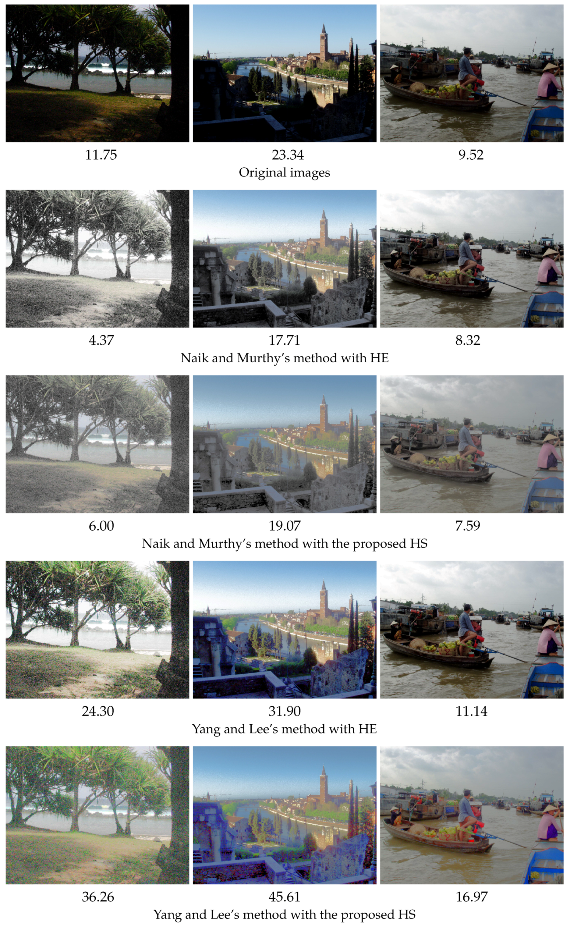
Figure 7 shows the results on the INRIA Holidays dataset [23,24], where the top row shows the original images, and the second to fifth rows show the results by Naik and Murthy’s method with HE and the proposed HS, and Yang and Lee’s method with HE and the proposed HS, respectively. The number under each image denotes the mean saturation value. The proposed HS improves the mean saturation of almost all examples except for an image with the mean saturation value 7.59, which is lower than 8.32 given by Naik and Murthy’s method with HE.
5. Discussion
In the above experimental results, we have compared four hue-preserving color image enhancement methods: Naik + HE, Naik + Proposed HS, Yang + HE and Yang + Proposed HS. First, we confirmed the fact that Naik and Murthy’s method does not increase the saturation of original colors experimentally. Next, we also experimentally confirmed the claim in Lemma 2, that is, Yang and Lee’s method can improve the saturation compared with Naik and Murthy’s method. Moreover, we demonstrated that the proposed HS method can improve the saturation compared with the conventional HE method used in both Naik and Murthy’s and Yang and Lee’s methods.
The target histogram for the proposed HS method is derived from the geometric shape of RGB color space, that is, a cube with a side length of 1, and has an analytic expression that can be integrated to obtain the cumulative target histogram used in the proposed HS. As a result, the proposed HS method has no additional assumptions or parameters. Therefore, there is no need for users to be bothered with any parameter settings. Additionally, the proposed HS method can suppress the contrast overenhancement that frequently occurs when HE is used.
Consequently, the proposed HS method can be used for an alternative method of HE because it is a parameter-free method as well as HE, and can enhance the color saturation compared with the conventional hue-preserving color image enhancement methods, while it can suppress the contrast overenhancement that occurs in HE frequently.
Acknowledgments
This work was supported by JSPS KAKENHI Grant Number JP16H03019.
Author Contributions
All of the authors contributed extensively to this work presented in the paper. Kohei Inoue has coordinated the work and participated in all section. Kiichi Urahama is an advisor guiding the designing of image processing methods. Kenji Hara provides suggestions to improve the algorithm and revise the whole paper.
Conflicts of Interest
The authors declare no conflict of interest.
Abbreviations
The following abbreviations are used in this manuscript:
| RGB | red, green and blue |
| CMY | cyan, magenta and yellow |
| HSI | hue, saturation and intensity |
| HE | histogram equalization |
| HS | histogram specification |
Appendix A. Proofs of Lemmas
In this section, we prove Lemmas 1 and 2 described above.
Proof of Lemma 1.
Proof of Lemma 2.
In Case (I), for , there are three cases of the position of corresponding to the left, middle and right: and . For , we have , from which it follows that . For , we have for , whose saturation is given by from Equation (3) in Lemma 1. We also have for , whose saturation is given by from Equation (2) in Lemma 1. Therefore, we have that or . For , we have and for , whose saturation is given by by Lemma 1. Therefore, we have that
or .
In Case (II), since Yang and Lee’s method outputs the same result as Naik and Lee’s method, we have immediately.
In Case (III), for , there are three cases of the position of corresponding to the left, middle and right: and . For , we have , whose saturation is given by . We also have for , whose saturation is given by . Therefore, we have that
or . For , we have and , whose saturation is given by . Therefore, we have
or . For , we have , whose saturation is given by , and , whose saturation is given by .
Consequently, holds in any case. ☐
References
- Anjana, N.; Jezebel Priestley, J.; Nandhini, V.; Elamaran, V. Color Image Enhancement using Edge Based Histogram Equalization. Indian J. Sci. Technol. 2015, 8, 1–6. [Google Scholar] [CrossRef]
- Mudigonda, S.P.; Mudigonda, K.P. Applications of Image Enhancement Techniques—An Overview. MIT Int. J. Comput. Sci. Inf. Technol. 2015, 5, 17–21. [Google Scholar]
- Sharo, T.A.; Raimond, K. A Survey on Color Image Enhancement Techniques. IOSR J. Eng. 2013, 3, 20–24. [Google Scholar] [CrossRef]
- Saleem, S.A.; Razak, T.A. Survey on Color Image Enhancement Techniques using Spatial Filtering. Int. J. Comput. Appl. 2014, 94, 39–45. [Google Scholar]
- Suganya, P.; Gayathri, S.; Mohanapriya, N. Survey on Image Enhancement Techniques. Int. J. Comput. Appl. Technol. Res. 2013, 2, 623–627. [Google Scholar] [CrossRef]
- Bisla, S. Survey on Hue-Preserving Color Image Enhancement without Gamut Problem. Int. J. Sci. Res. 2017, 6, 1911–1914. [Google Scholar]
- Zhang, X.; Xin, Y.; Huang, H.; Xie, N. Color Image Enhancement Using Optimal Linear Transform with Hue Preserving and Saturation Scaling. Int. J. Intell. Eng. Syst. 2015, 8, 1–9. [Google Scholar] [CrossRef]
- Aashima; Verma, N. Hue Preserving Improvement in Quality of Colour Image. Int. J. Adv. Res. Eng. Technol. 2016, 4, 1–5. [Google Scholar]
- Porwal, D.; Alam, M.S.; Porwal, A. HUE Preserving Color Image Enhancement without GAMUT Problem using newly proposed Algorithm. Int. J. Eng. Comput. Sci. 2013, 2, 3450–3454. [Google Scholar]
- Chien, C.-L.; Tseng, D.-C. Color Image Enhancement with Exact HSI Color Model. Int. J. Innov. Comput. Inf. Control 2011, 7, 6691–6710. [Google Scholar]
- Gorai, A.; Ghosh, A. Hue-preserving color image enhancement using particle swarm optimization. In Proceedings of the IEEE Recent Advances in Intelligent Computational Systems (RAICS), Trivandrum, India, 22–24 September 2011; pp. 563–568. [Google Scholar]
- Taguchi, A. Color Systems and Color Image Enhancement Methods. ECTI Trans. Comput. Inf. Technol. 2016, 10, 97–110. [Google Scholar]
- Menotti-Gomes, D.; Najman, L.; Facon, J.; De Araújo, A.A. Fast Hue-Preserving Histogram Equalization Methods for Color Image Contrast Enhancement. Int. J. Comput. Sci. Inf. Technol. 2012, 4, 243–259. [Google Scholar]
- Pierre, F.; Aujol, J.-F.; Bugeau, A.; Steidl, G.; Ta, V.-T. Hue-preserving perceptual contrast enhancement. In Proceedings of the IEEE International Conference Image Process, Phoenix, AZ, USA, 25–28 September 2016. [Google Scholar]
- Nikolova, M.; Steidl, G. Fast Hue and Range Preserving Histogram Specification: Theory and New Algorithms for Color Image Enhancement. IEEE Trans. Image Process. 2014, 23, 4087–4100. [Google Scholar] [CrossRef] [PubMed]
- Nikolova, M.; Steidl, G. Fast Ordering Algorithm for Exact Histogram Specification. IEEE Trans. Image Process. 2014, 23, 5274–5283. [Google Scholar] [CrossRef] [PubMed]
- Naik, S.K.; Murthy, C.A. Hue-preserving color image enhancement without gamut problem. IEEE Trans. Image Process. 2003, 12, 1591–1598. [Google Scholar] [CrossRef] [PubMed]
- Han, J.-H.; Yang, S.; Lee, B.-U. A novel 3-d color histogram equalization method with uniform 1-d gray scale histogram. Trans. Image Process. 2011, 20, 506–512. [Google Scholar] [CrossRef] [PubMed]
- Yang, S.; Lee, B. Hue-preserving gamut mapping with high saturation. Electronics Letters 2013, 49, 1221–1222. [Google Scholar] [CrossRef]
- Gonzalez, R.C.; Woods, R.E. Digital Image Processing, 3rd ed.; Prentice-Hall, Inc.: Upper Saddle River, NJ, USA, 2006. [Google Scholar]
- Inoue, K.; Hara, K.; Urahama, K. On hue-preserving saturation enhancement in color image enhancement. IEICE Trans. Fundam. 2015, 98, 927–931. [Google Scholar] [CrossRef]
- The Standard Image Data-BAse (SIDBA). Available online: http://www.ess.ic.kanagawa-it.ac.jp/app_images_j.html (accessed on 30 June 2017).
- Jegou, H.; Douze, M.; Schmid, C. Hamming Embedding and Weak Geometry Consistency for Large Scale Image Search. In Proceedings of the 10th European Conference on Computer Vision, Marseille, France, 12–18 October 2008. [Google Scholar]
- The INRIA Holidays Dataset. Available online: http://lear.inrialpes.fr/~jegou/data.php (accessed on 30 June 2017).
Figure 1.
Cross sections of RGB color cube with equiintensity planes, , where denotes a point on the plane: (a) ; (b) ; (c) .
Figure 1.
Cross sections of RGB color cube with equiintensity planes, , where denotes a point on the plane: (a) ; (b) ; (c) .
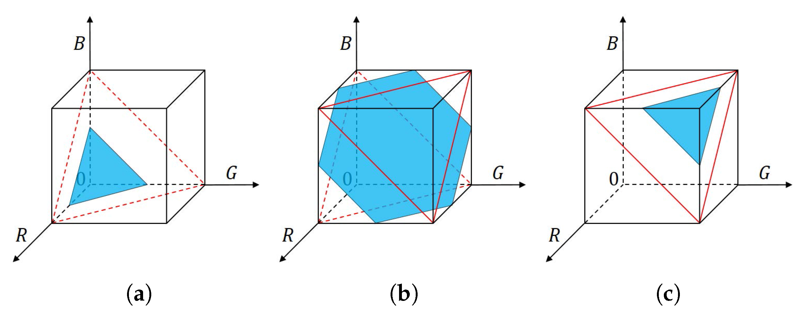
Figure 2.
Area of cross section of RGB color cube and equiintensity plane, , and its integral, .
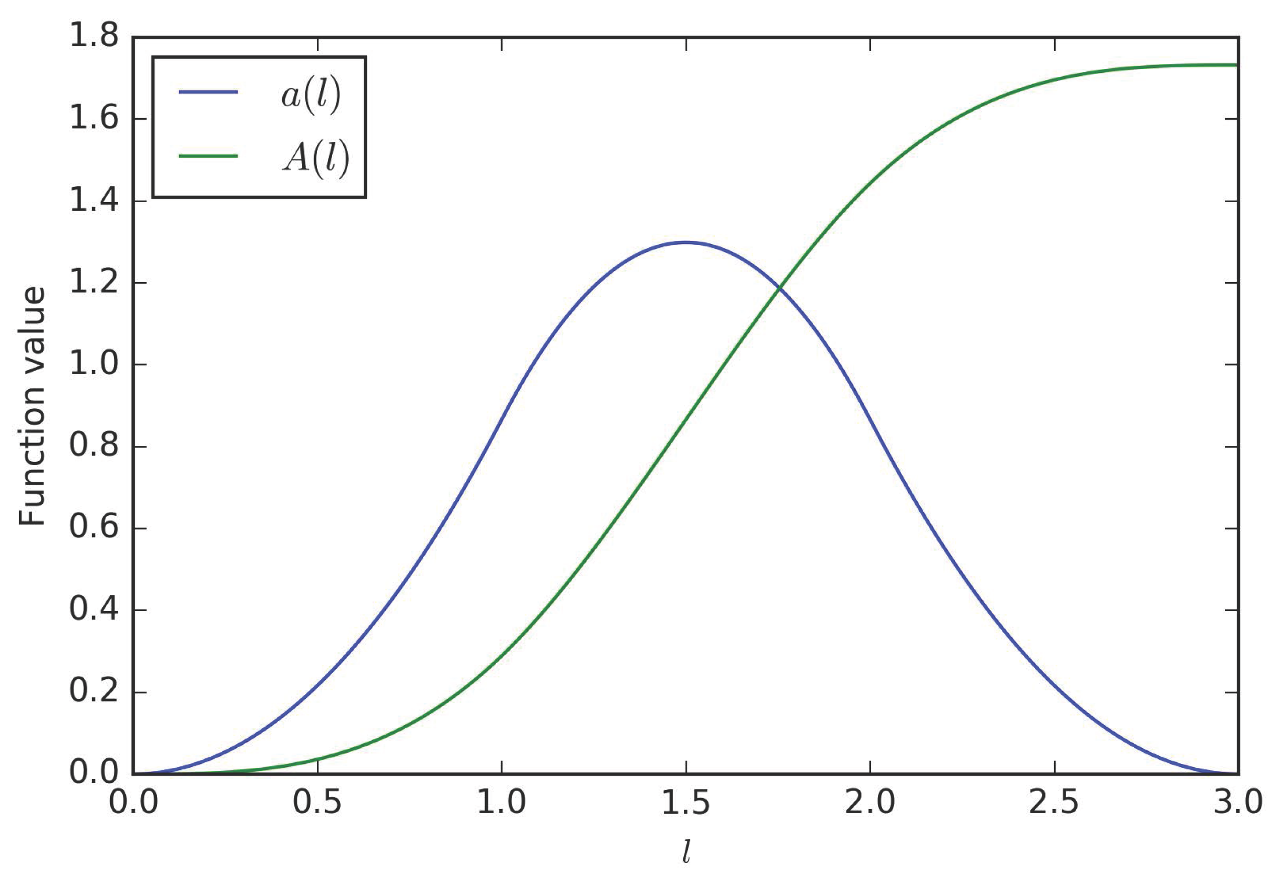
Figure 3.
Results of hue-preserving color image enhancement.

Figure 4.
Saturation images.
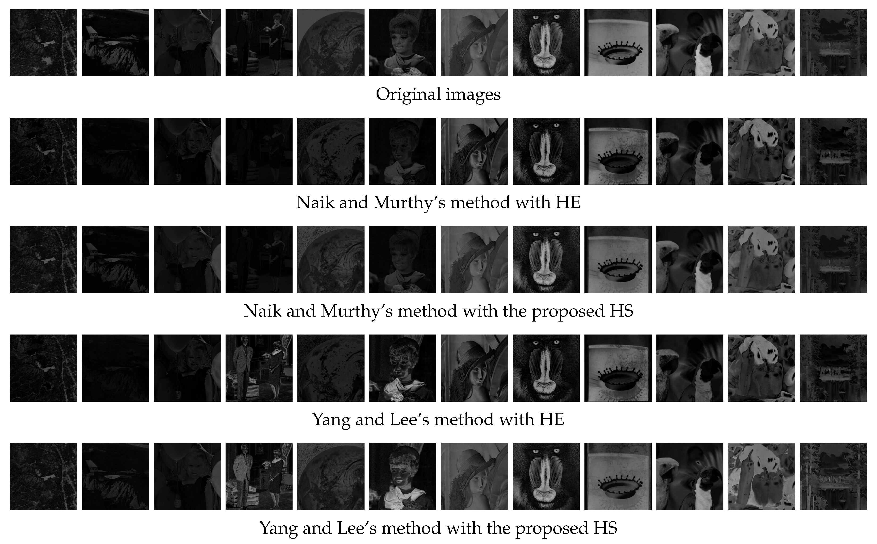
Figure 5.
Difference maps of saturation images.
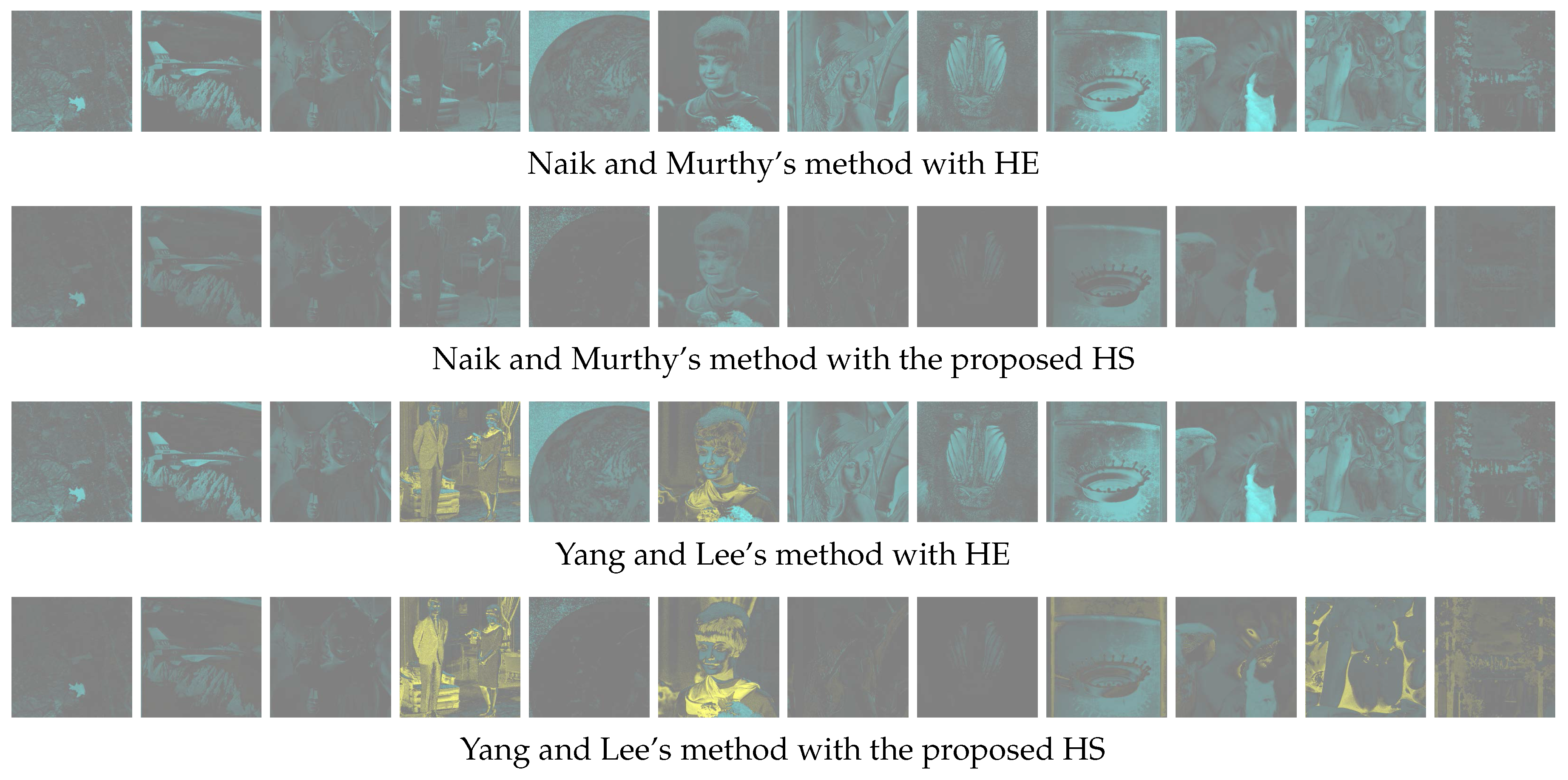
Figure 6.
Mean saturation.
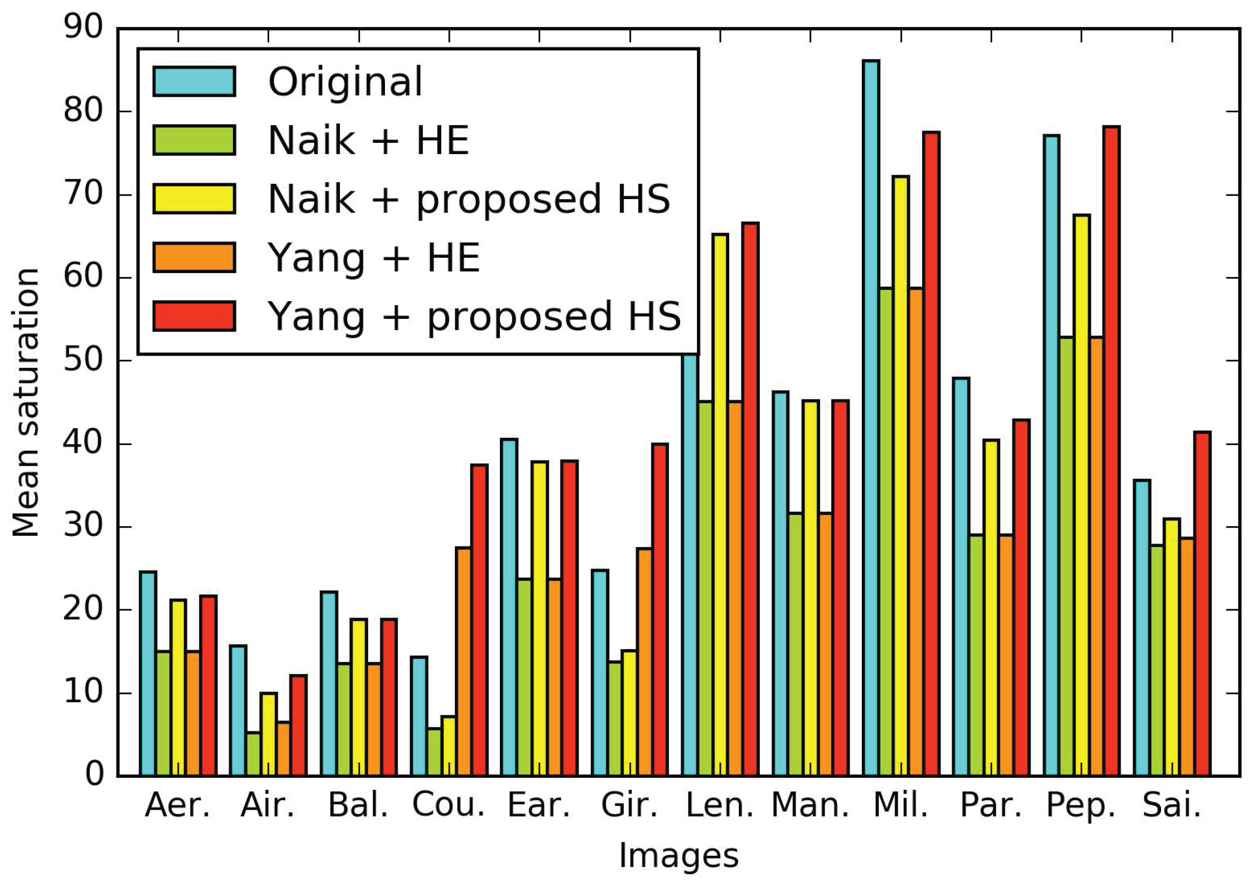
Figure 7.
Results on the INRIA (Institut National de Recherche en Informatique et en Automatique) dataset with the mean saturation values.
Figure 7.
Results on the INRIA (Institut National de Recherche en Informatique et en Automatique) dataset with the mean saturation values.


Table 1.
Total mean saturation. In this table, ’Original’ means the original images, ’Naik+HE’ means Naik and Murthy’s method with HE, ’Naik+Proposed HS’ means Naik and Murthy’s method with the proposed HS, ’Yang+HE’ means Yang and Lee’s method with HE, and ’Yang+Proposed HS’ means Yang and Lee’s method with the proposed HS.
| Original | Naik + HE | Naik + Proposed HS | Yang + HE | Yang + Proposed HS |
|---|---|---|---|---|
| 41.89 | 26.84 | 35.98 | 29.97 | 43.31 |
© 2017 by the authors. Licensee MDPI, Basel, Switzerland. This article is an open access article distributed under the terms and conditions of the Creative Commons Attribution (CC BY) license (http://creativecommons.org/licenses/by/4.0/).
Share and Cite
MDPI and ACS Style
Inoue, K.; Hara, K.; Urahama, K. RGB Color Cube-Based Histogram Specification for Hue-Preserving Color Image Enhancement. J. Imaging 2017, 3, 24. https://doi.org/10.3390/jimaging3030024
AMA Style
Inoue K, Hara K, Urahama K. RGB Color Cube-Based Histogram Specification for Hue-Preserving Color Image Enhancement. Journal of Imaging. 2017; 3(3):24. https://doi.org/10.3390/jimaging3030024
Chicago/Turabian StyleInoue, Kohei, Kenji Hara, and Kiichi Urahama. 2017. "RGB Color Cube-Based Histogram Specification for Hue-Preserving Color Image Enhancement" Journal of Imaging 3, no. 3: 24. https://doi.org/10.3390/jimaging3030024
Note that from the first issue of 2016, this journal uses article numbers instead of page numbers. See further details here.