Using SEBAL to Investigate How Variations in Climate Impact on Crop Evapotranspiration

Abstract

Water allocation to crops, and especially to the most water intensive ones, has always been of great importance in agricultural processes. Deficit or excessive irrigation could create either crop health-related problems or water over-consumption, respectively. The latter could lead to groundwater depletion and deterioration of its quality through deep percolation of agrichemical residuals. In this context, and under the current conditions where Cyprus is facing effects of possible climate changes, the purpose of this study seeks to estimate the needed crop water requirements of the past (1995–2004) and the corresponding ones of the present (2005–2015) in order to test if there were any significant changes regarding the crop water requirements of the most water-intensive trees in Cyprus. The Mediterranean region has been identified as the region that will suffer the most from variations of climate. Thus the paper refers to effects of these variations on crop evapotranspiration (ETc) using remotely-sensed data from Landsat TM/ETM+/OLI employing a sound methodology used worldwide, the Surface Energy Balance Algorithm for Land (SEBAL). Though the general feeling is that of changes on climate will consequently affect ETc, our results indicate that there is no significant effect of climate variation on crop evapotranspiration, despite the fact that some climatic factors have changed. Applying Student’s t-test, the mean values for the most water-intensive trees in Cyprus of the 1994–2004 decade have shown no statistical difference from the mean values of 2005–2015 for all the cases, concluding that the climate change taking place in the past decades in Cyprus have either not affected the crop evapotranspiration or the crops have managed to adapt to the new environmental conditions through time.

1. Introduction

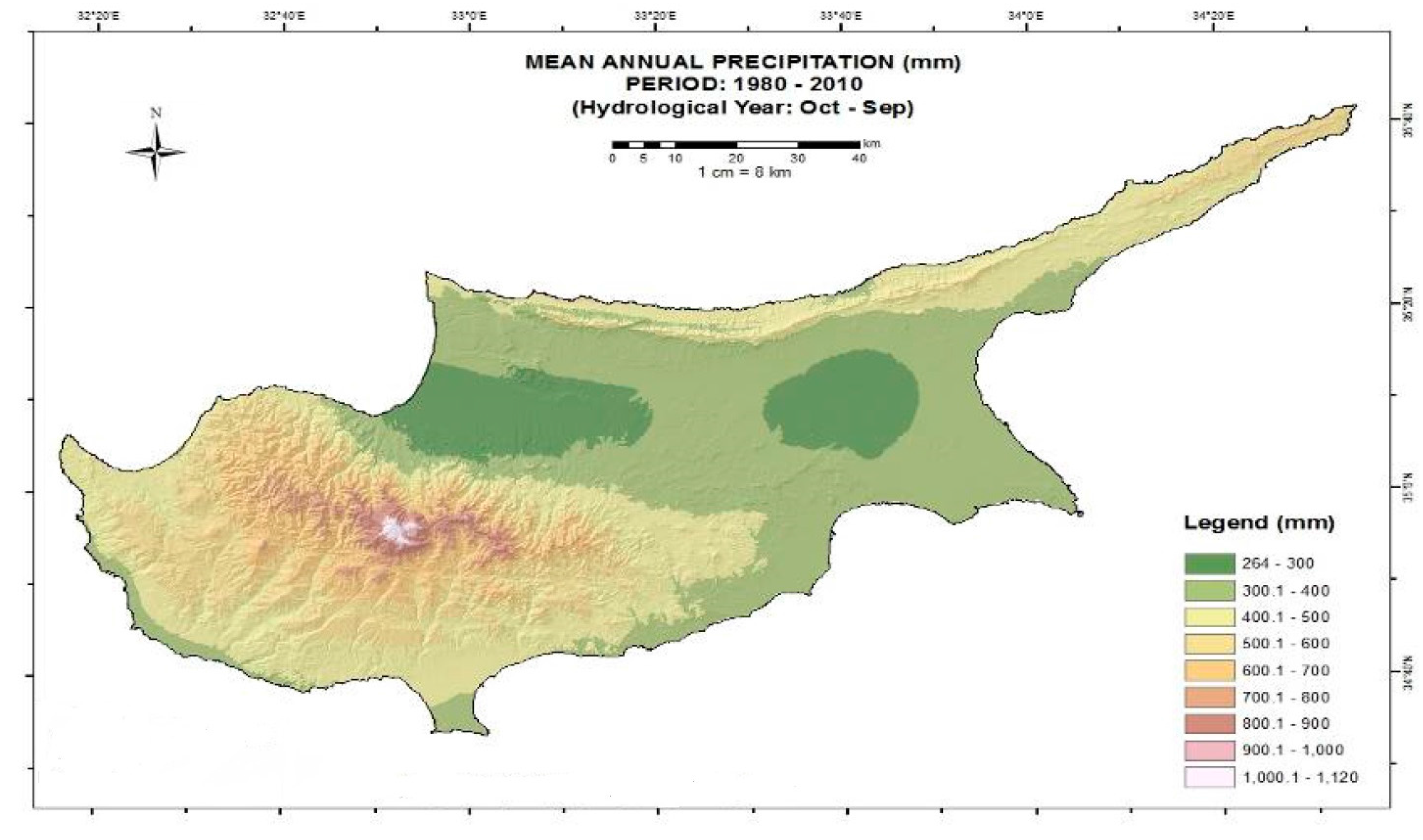
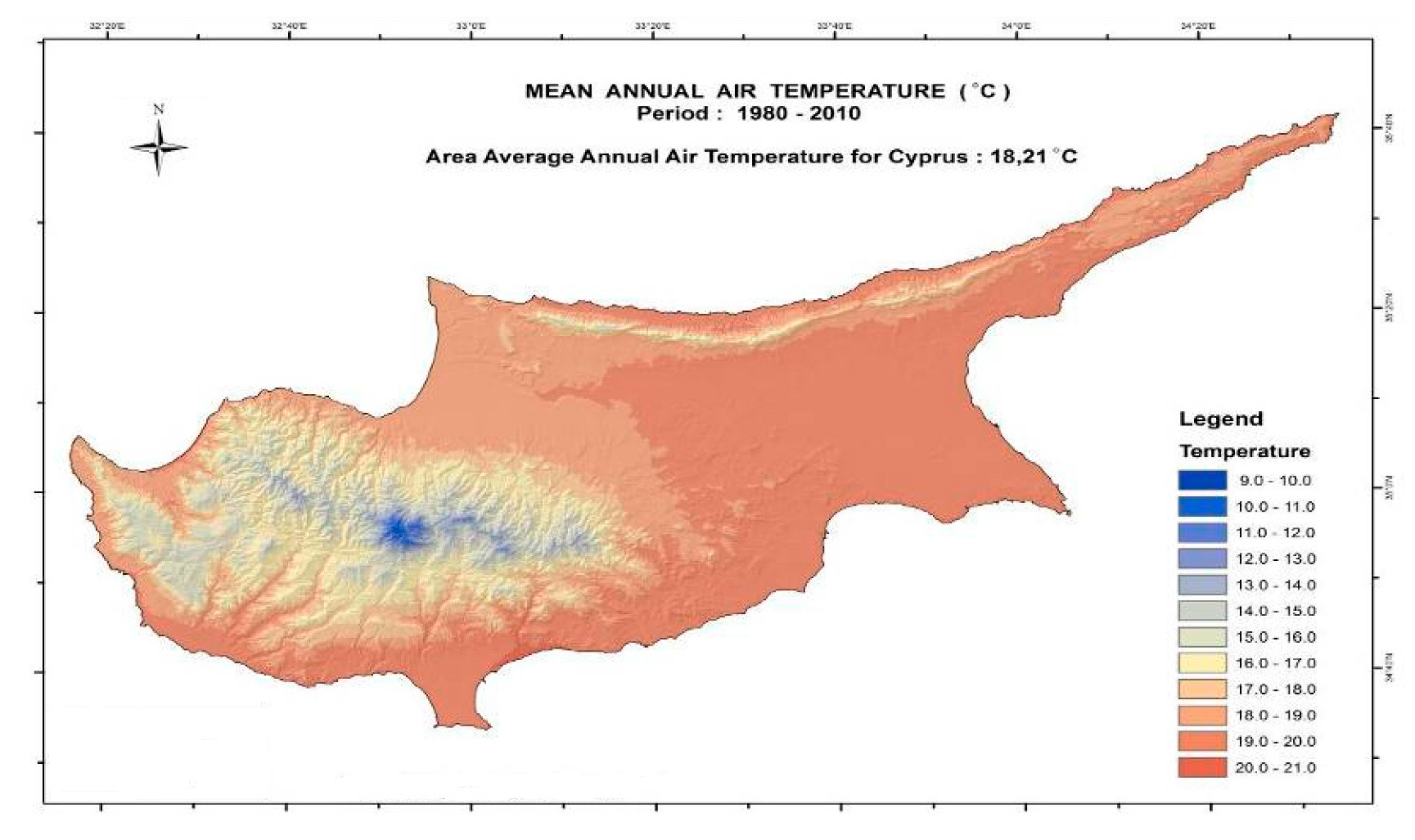
1.1. Climate and Climate Changes in Cyprus

Cyprus has an intense Mediterranean climate with typical seasonal changes with hot, dry summers from mid-May to mid-September and rainy winters from mid-November to mid-March, which are separated by short autumn and spring seasons. In the summer, Cyprus is mainly under the influence of a shallow trough of low pressure extending from the high continental depression centered over Southwest Asia. It is a season of high temperatures with, usually, cloudless skies.

Climate change could lead to serious socioeconomic consequences for Europe in the long term but some effects, such as an increasing frequency of extreme events and weather disasters, will be felt in the short term [1] (

Table 1. Simplified summary of climate change impacts in Europe and their intensity.

Climate Change Indicators	Northern Europe	Central and Eastern Europe	Mediterranean
Direct losses from weather disasters	M(−)	M(−)	H(−)
River flooding disasters	M(−)	H(−)	L(−)
Coastal flooding	H(−)	M(−)	H(−)
Public water supply and drinking water	L(−)	L(−)	H(−)
Crop yields in agriculture	H(+)	M(−)	H(−)
Crop yields in forestry	M(+)	L(−)	H(−)
Biodiversity	M(+)	M(−)	H(−)
Energy for heating and cooling	M(+)	L(+)	M(−)
Hydropower and cooling for thermal plants	M(+)	M(−)	H(−)
Tourism and recreation	M(+)	L(+)	M(−)
Health	L(−)	M(−)	H(−)

Notes: H: High; M: Medium; L: Low; (+): Positive impact; (−): Negative impact.

). At the same time, the impacts of climate change will vary across European regions, and sometimes from even one member state to another. The three large climatic zones in Europe (meaning Northern, Central, and Mediterranean regions) will, therefore, need different regional responses [1]. Along with the mixed physical impacts in each region, various sectors will be affected in different ways.

Cyprus has seen a decrease in precipitation in the recent past. A regional analysis of the changes in precipitation found a statistically significant step change in the 1916–2000 annual precipitation time series between the hydrologic years 1968/1969 and 1971/1972, with a 15–25% reduction in precipitation for the last 40 years [2]. Data from the Cyprus Meteorological Service gives an average annual precipitation over the government-controlled area of Cyprus of 541 mm for 1901/1902–1969/1970 and 466 mm for the 1970/1971–2009/2010 period [2]. This decrease in precipitation has resulted in an even greater decrease in the country’s water resources. Considering that the majority of Cyprus’ dams and irrigation projects have been designed on the basis of precipitation data from a wetter past, they have not always lived up to the expectations they raised (Figure 1).

Temperatures are high in summer and the mean daily temperature in July and August range between 22 °C on the Troodos Mountains and 29 °C on the central plain, while the average maximum temperature for these months ranges between 27 and 36 °C, respectively (Figure 2). Winters are mild with a mean January temperature of 3 °C on the higher parts of the Troodos Mountains and 10 °C on the central plain. Sunshine is abundant during the whole year, and particularly from April to September when the average duration of sunshine exceeds 11 h per day while, sometimes, the yearly sunshine period exceeds 300 days. Winds are generally light to moderate and variable in direction. Strong winds may occur sometimes, but gales are infrequent over Cyprus and are mainly confined to exposed coastal areas, as well at areas with high elevation [3,4].

Recent studies by the Ministry of Agriculture, Natural Resources, and Environment [4,5] and other research institutes [3,6,7] which refer to the climate change in agricultural terms in Cyprus, indicated that climate change is likely to increase irrigation water demands, reduce yields, and increase soil degradation. This means less water use for agriculture, which will also come at a higher price. These studies have shown that there is highly variable nature of the climate in Cyprus, both in space and in time. Statistically significant increasing trends were found for the minimum and maximum temperatures. Analysis of the crop areas of the past in Cyprus showed a very large reduction in the harvested areas of main traditional crops cultivated on the island. The area planted with seasonal crops fluctuated between dry and wet years but, overall, remained fairly stable, while irrigation has an important effect on reducing the variability in total annual production. Nevertheless it is important to mention that there is the possibility to reuse an important amount of reclaimed water which is used directly in the agricultural sector.

Climate change projections extracted from the specific studies with case scenarios showed a clear increase in temperature, while trends in precipitation are masked by the highly-variable nature of the precipitation. However, a reduction of 2–8% has been projected for 2026–2050, relative to 1976–2000. Analysis of two possible climate change scenarios, represented by more dry years, higher evaporative demand, and less irrigation water supply, which resulted in a reduction of the irrigated area by 25%, projected a possible reduction of 41–43% in total national crop production for the future.

1.2. Crop Water Requirements

Water requirements for each crop are inferred by the crop’s evapotranspiration (ETc). Evapotranspiration (ET) is the loss of water from a vegetative surface through the combined processes of plant transpiration and soil evaporation. Since ETc is directly dependent on meteorological factors such as radiation, air temperature, humidity, and wind speed, along with crop parameters (FAO), one could expect that there would be a change on the water requirements of crops due to possible climate change, or since climate change is still a controversial term, authors would better say variations of climate. There is no bound method to obtain an accurate measure of ETc due to the variability and complexity of climatic factors and biophysical variables involved in the process. Evapotranspiration (ET) estimation is important for hydrologic modeling and irrigation scheduling [6,7,8].

Actual evapotranspiration ET_a is one of the most useful indicators to explain whether the water is used as “intended” or not. ET_a variations, both in space and time, and from different land use classes, are thought to be highly indicative for the adequacy, reliability, and equity in water use; the knowledge of these terms is essential for judicious water resources management. Unfortunately, ET_a estimation under actual field conditions is still a very challenging task for scientists and water managers. The complexity associated with the estimation of ET has led to the development of various methods for estimating this parameter over time [9,10].

Remote sensing-based agro-meteorological models are presently most suited for estimating crop water use at both field and regional scales [11]. Numerous ET algorithms have been developed to make use of remote sensing data acquired by sensors on airborne and satellite platforms [12]. This study demonstrates the application of a remote sensing algorithm, the Surface Energy Balance Algorithm for Land (SEBAL) [11,13,14] that is applied employing the necessary modifications and adaptations regarding the crop canopy parameters such as Leaf Area Index and Crop Height. The SEBAL model has been used in several studies [15,16,17,18,19,20,21]. SEBAL has been applied in several countries of the Mediterranean region. It has been applied in Egypt [20] and then in Turkey [13], in Greece [22,23], and also in Cyprus [19,20,21].

ETc in the study area was firstly estimated by applying the Surface Energy Balance Algorithm for Land (SEBAL) on the satellite images which included a thermal band (Landsat images). SEBAL is a thermodynamically-based model, using the partitioning of sensible heat flux and latent heat of vaporization flux as described by [15], who developed the algorithm. In the SEBAL model, ETc is computed from satellite images and weather data using the surface energy balance. Remotely-sensed data in the visible, near-infrared, and thermal infrared bands are used to derive the energy balance components along with ground measured solar radiation, if available. The other ground measurements that are required as model inputs are air temperature, relative humidity, and wind speed at a point within the image.

SEBAL has an internal calibration for removing atmospheric effects using a series of iteration on Sensible Heat Flux (H) [15,16,17,18,19,20,21]. Since the satellite image provides information for the overpass time only, SEBAL computes an instantaneous ET flux for the image time. The ET flux is calculated for each pixel of the image as a “residual” of the surface energy budget equation:

$$\lambda ET=R_n-G-H$$

(1)

where:

▪

R_n is the instantaneous net radiation (W∙m⁻²)

▪

G is the instantaneous soil heat flux (W∙m⁻²)

▪

H is the instantaneous sensible heat flux (W∙m⁻²)

▪

λET is the instantaneous latent heat flux (W∙m⁻²)

In Equation (1), the soil heat flux (G) and sensible heat flux (H) are subtracted from the net radiation flux at the surface (R_n) to compute the “residual” energy available for evapotranspiration (λET) (Equation (1)). Soil heat flux is empirically calculated using vegetation indices, surface temperature and surface albedo. Sensible heat flux is computed using wind speed observations, estimated surface roughness and surface to air temperature differences. SEBAL uses an iterative process to correct for atmospheric instability due to the buoyancy effects of surface heating. Once the latent heat flux (λET) is computed for each pixel, an equivalent amount of instantaneous ET (mm/h) is readily calculated by dividing by the latent heat of vaporization (λ). Then, daily ETc is inferred.

In this paper, the actual crop evapotranspiration of the most water-intensive crops of Cypriot agriculture (citrus, bananas, colocasi, potatoes, and avocado trees) was determined as the residual of the energy balance equation using the measured net radiation (R_n), the soil heat flux density (G), and the estimated sensible heat flux density (H). There are three main agricultural areas of the island where the specific trees and annual crops are cultivated. The plots cultivated with the specific species are experimental plots cultivated with the same plots every year, from the Agricultural Research Institute of Cyprus. The objective of this paper is to compare the mean ETc values of the period 1994–2004 to the corresponding ones of the period 2005–2015, applying the same methodology (SEBAL) and satellite images from a single satellite system, namely LANDSAT. Unfortunately the satellite archive used had only images since 1994 so the authors had to choose two decades to compare the ETc of each crop. Meteorological data regarding the specific years were used, so as to retrieve the mean ETc values. The meteorological data were taken from specific stations, based on the three main agricultural areas mentioned earlier as shown in Figure 3 (No. 41 for Polis, No. 82 for Pafos, and No. 845 for Famagusta). All three meteorological stations are automatic and climatological and are constantly calibrated by the Cyprus Meteorological Service to whom they belong. All details about the method retrieving the meteorological data can be found at http://www.moa.gov.cy/moa/ms/ms.nsf/All/257A48DEA21CDAC4C22576C80036FB64?OpenDocument.

2. Materials and Methods

The method focuses on the SEBAL application for estimating the actual crop evapotranspiration of the specific crops in Cyprus during the two periods, namely 1994–2004 and 2005–2015. The goal is to create monthly average data for these two periods for all the crops included in this study.

The SEBAL model is applied for estimating the crop evapotranspiration using remotely-sensed data. The specific algorithm is applied to satellite images of the past referring to the 1994–2004 decade and, at the same time, to satellite images of the last decade, 2005–2015. As mentioned earlier only Landsat images were used in order to be consistent in the methodology. Landsat 5TM, seven ETM+, and eight OLI images with 15 m spatial resolution and 16-day temporal resolution of the island were used and transformed into ET_a maps. Then, employing these maps, the necessary crop water requirements for each crop were inferred and recorded for the two periods under investigation. Average values for each month in mm have been found and compared for the two periods in order to statistically test if there is any significant difference on crop water requirements for each crop, between the periods denoting that the climate variations have affected the crop water requirements of the most water-intensive crops in Cyprus.

SEBAL computes a complete radiation and energy balance along with the resistances for momentum, heat, and water vapor transport for each pixel [8,9]. The key input data for SEBAL consists of spectral radiance in the visible, near-infrared, and thermal infrared parts of the spectrum. Thus, the model can be applied using satellite sensors having a thermal band. Landsat 5 and 7 images were used in this study. In addition to satellite images, the SEBAL model requires weather parameters (wind speed, humidity, solar radiation, air temperature). These meteorological parameters were used as inputs for the algorithm and they were provided from the national meteorological station next to the area of interest. Evaporation was calculated from the instantaneous evaporative fraction, and the daily averaged net radiation, R_n24. The evaporative fraction was computed from the instantaneous surface energy balance at satellite overpass on a pixel-by-pixel basis:

$$\lambda E=R_n-(G_0+H)$$

(2)

where λE is the latent heat flux (W m⁻²), R_n is the net radiation (W m⁻²), G₀ is the soil heat flux (W m⁻²), and H is the sensible heat flux (W m⁻²) as shown in Equation (2).

The latent heat flux describes the amount of energy consumed to maintain a certain crop evaporation rate. The surface albedo, surface temperature and vegetation index are derived from satellite spectral measurements, and are used together to solve R_n, G₀ and H. The instantaneous latent heat flux, λE, is the calculated residual term of the energy budget, and it is then used to compute the instantaneous evaporative fraction Λ (Equation (3)):

$$\mathrm{\Lambda }=\frac{\lambda E}{\lambda E+H}=\frac{\lambda E}{R_n-G_0}$$

(3)

The instantaneous evaporative fraction Λ expresses the ratio of the actual to the crop evaporative demand when the atmospheric moisture conditions are in equilibrium with the soil moisture conditions. The instantaneous value can be used to calculate the daily value because the evaporative fraction tends to be constant during daytime hours, although the H and λE fluxes vary considerably [19,24]. The difference between the instantaneous evaporative fraction at satellite overpass and the evaporative fraction derived from the 24-h integrated energy balance is marginal and may be neglected [19,25,26]. For time scales of one day or longer, G₀ can be ignored and the net available energy (R_n − G₀) reduces to net radiation (R_n). At daily timescales, ET₂₄ (mm/day) can be computed as (Equation (4)):

$$E{T}_{24}=\frac{86,400\times {10}^3}{\lambda {\rho }_w}\mathrm{\Lambda }{R}_{n24}$$

(4)

where R_n24 (W m²) is the 24-h averaged net radiation, λ (J kg⁻¹) is the latent heat of vaporization, and ρ_w (kg m⁻³) is the density of water.

LAI map. For estimating LAI the following equation was applied [19] (Equation (5)):

$$LAI=-\raisebox{1ex}{$1$}\!\left/ \!\raisebox{-1ex}{$\alpha $}\right.\ln \left(1-\frac{WDVI}{{\rho }_{\infty }({\lambda }_{NIR)}}\right)$$

(5)

where:

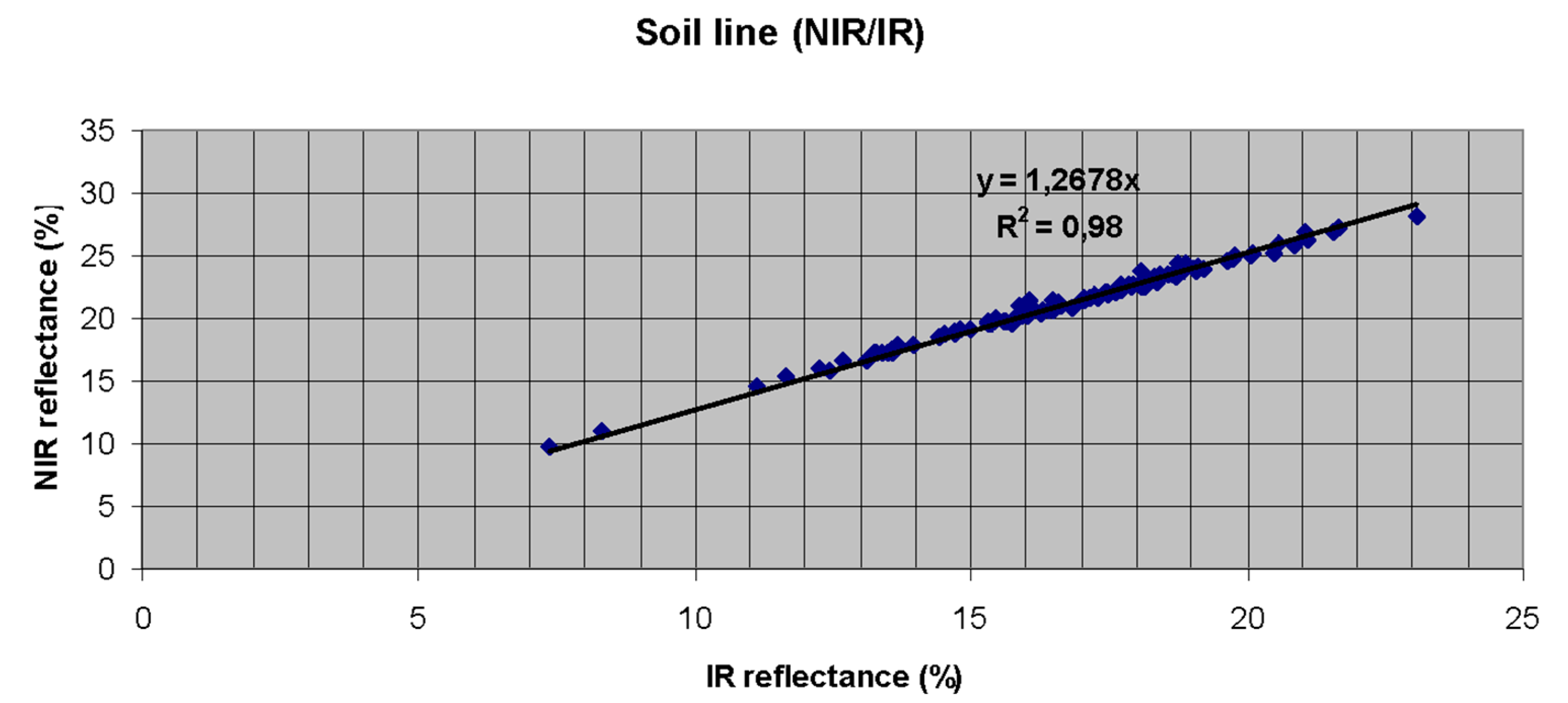
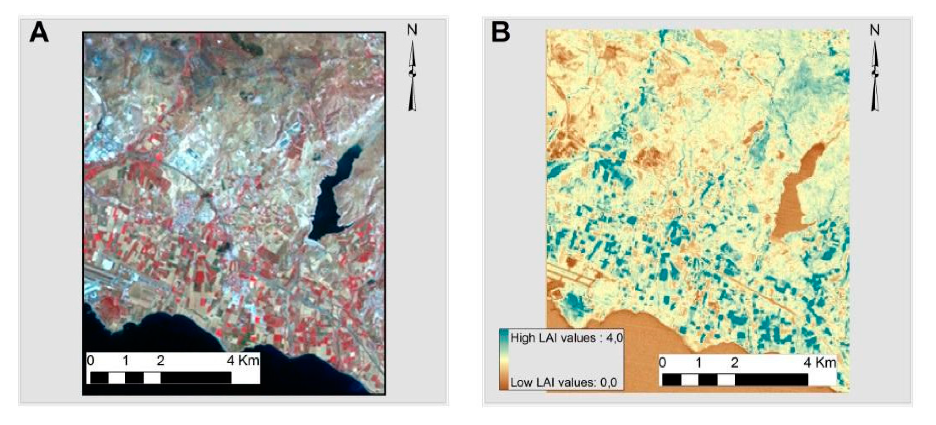
• LAI = Leaf Area Index;
• WDVI = Weighted Difference Vegetation Index;
• α = complex combination of extinction and scattering coefficients; and
• ρ_∞ = asymptotically limiting value of the WDVI at very high LAI values.

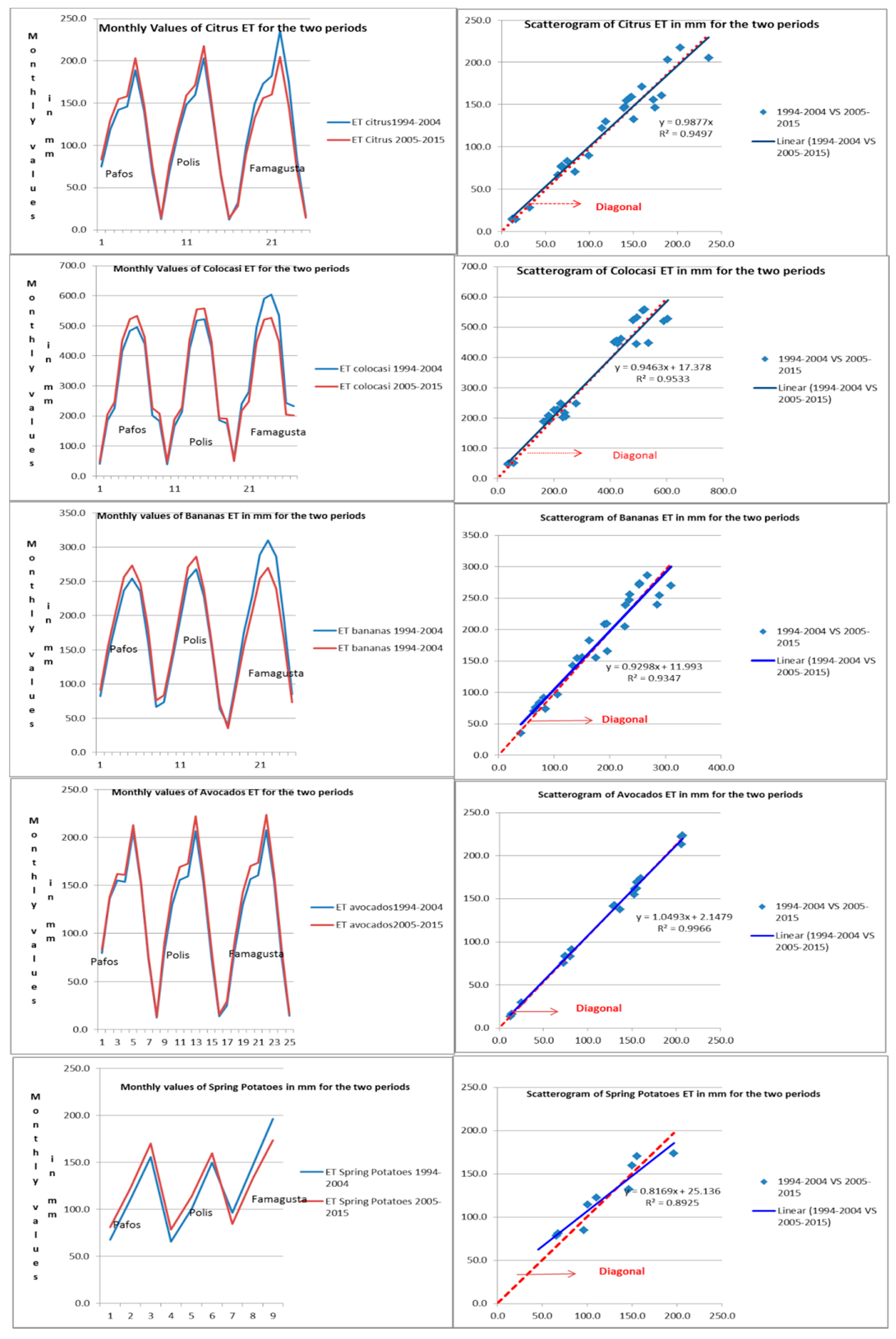
Standard values for α and ρ_∞ were taken from literature specifically for annual crops and trees correspondingly.

As WDVI is a distance based index, relatively better atmospheric correction needs to be applied to the data, which is not necessary for ratio based indices, like NDVI and SAVI. However, using a spectroradiometer, as mentioned before, this limitation is bypassed. The Weighted Difference Vegetation Index (WDVI) is defined as follows (Equation (6)):

WDVI = NIR-γR

(6)

where NIR is the reflectance of near-infrared band, RED is the reflectance of visible red band, and γ is the slope of the soil line [13,14,15]. The WDVI index has the advantage to reduce the influence of soil background on the surface reflectance values to a great extent. Although simple, WDVI is as efficient as most of the slope-based VI. The effect of weighting the red band with the slope of the soil line is the maximization of the vegetation signal in the near-infrared band and the minimization of the effect of soil brightness. After creating a set of data from bare soil of the area during the year, the slope of the line was set to 1.27. The slope line is created from the NIR(Y axis in Figure 4) and R (X axis in Figure 4) spectra using spectroradiometric data (200 sample random measurements) from the areas’ soil. (Figure 4).

The specific Equation (5) was applied to satellite images, and LAI maps were created. Various studies have shown that empirical equations of LAI and vegetation indices can provide good estimates of LAI from the satellite images. Then the LAI maps were used as inputs for the SEBAL algorithm for inferring the crop evapotranspiration for each crop or tree, as displayed in Figure 5.

In the procedure for applying SEBAL algorithm, a crucial point is the selection of the two ‘anchor’ pixels, the ‘hot’ and the ‘cold’ pixels, in the area of interest. These two pixels are used to find the difference (dT) of the temperature between the surface temperature (Ts) and the air temperature (near the surface), which is a basic assumption that SEBAL relies on. It is assumed that a linear relationship connects the Ts and the dT in the form of (Equation (7)):

dT = aTs + b

(7)

The linear equation above is developed by using the dT values for the cold and hot pixels and the surface temperature [15,19,27,28]. The cold pixel in SEBAL is used to define the amount of ETc, through H, occurring from the most vegetated and well-watered areas of the image. Usually, an alfa-alfa cultivation or water body is used to identify cold pixels in the area of interest. Surface temperature (Ts) (cold temperature), albedo values (0.22–0.24), and LAI (LAI > 3) values are the combination that was used to identify the ‘cold’ pixel in the area of interest from vegetated areas in the image. The ‘hot’ pixel is a pixel where ETc should be zero. This pixel is usually located in dry, bare agricultural fields. Both of these “anchor” pixels should be located in large and homogeneous areas that contain more than one pixel of Landsat’s thermal band. The anchor cold and hot pixels in this thesis were selected in the area of interest where the cold pixel was located in lucerne under center pivot irrigation systems. The hot pixels were always found on bare soil surfaces.

Finally a statistical method for comparing the paired values for each crop of ETc (average monthly) has been employed, in order to test if there are significant differences among the different pairs. Student’s t-test is used to find out if there is a statistically significant difference between average monthly value of each crop for the 1994–2004 decade and the corresponding one of the 2005–2015 value. The Student’s t-test for paired samples, as a statistical significance test, was applied to compare and assess the results meaning. To assess the value of t, the standard deviation S_D of each pair of values (real and predicted) must be known. D_j refers to the difference of each pair, Da is the average difference of each pair, and n is the number of the pairs. Variance ($S_D^2$) is calculated from Equation (8):

$$s_D^2=\left[\Sigma D_j^2-\frac{{(\Sigma D_j)}^2}{n}\right]/\left(n-1\right)$$

(8)

Following, the average variance ($S_D^2$) of all pairs must be calculated from the following equation (Equation (9)):

$$s_{Da}^2=s_D^2/n$$

(9)

Finally, the t value is calculated solving Equation (10):

$$t=\frac{Da}{S_{Da}}$$

(10)

The comparison of results will illustrate that. If the null hypothesis is not rejected, then there is no statistically significant difference for the actual crop evapotranspiration.

3. Results

After the methodology deployment, the necessary data has been recorded in tables for each crop or tree. Actual crop evapotranspiration has been retrieved from the ETc maps produced from the SEBAL application for each month as shown in

Table 2. Average monthly ETc values for each crop for the Pafos area.

Pafos	Citrus		Colocasi		Bananas		Spring Potatoes		Avocado
	ET Crop (mm)		ET Crop (mm)		ET Crop (mm)		ET Crop (mm)		ET Crop (mm)
Month	1994–2004	2005–2015	1994–2004	2005–2015	1994–2004	2005–2015	1994–2004	2005–2015	1994–2004	2005–2015
January	0.0	0.0	0.0	0.0	0.0	0.0	0.0	0.0	0.0	0.0
February	0.0	0.0	0.0	0.0	0.0	0.0	0.0	0.0	0.0	0.0
March	0.0	0.0	41.4	49.3	0.0	0.0	67.8	80.9	0.0	0.0
April	74.8	83.0	184.1	204.5	82.1	91.1	110.4	122.6	79.9	82.9
May	118.4	129.5	225.9	247.1	141.3	154.6	155.5	170.1	136.4	137.6
June	142.4	154.7	415.3	451.3	191.5	208.0	0.0	0.0	155.3	161.8
July	145.9	157.9	482.8	522.6	236.5	256.0	0.0	0.0	153.9	160.8
August	188.9	203.1	495.3	532.6	254.3	273.4	0.0	0.0	206.1	213.0
September	140.5	147.5	439.7	461.5	235.2	246.8	0.0	0.0	152.5	154.6
October	68.0	76.1	202.0	226.1	163.0	182.5	0.0	0.0	72.7	75.5
November	12.8	14.6	182.8	208.1	66.7	75.9	0.0	0.0	12.5	13.2
December	0.0	0.0	0.0	0.0	0.0	0.0	0.0	0.0	0.0	0.0
Total	891.6	966.4	2669.3	2903.1	1370.5	1488.4	333.7	373.6	969.3	999.4

,

Table 3. Average monthly ETc values for each crop for the Polis area.

Polis	Citrus		Colocasi		Bananas		Spring Potatoes		Avocado
	ET Crop (mm)		ET Crop (mm)		ET Crop (mm)		ET Crop (mm)		ET Crop (mm)
Month	1994–2004	2005–2015	1994–2004	2005–2015	1994–2004	2005–2015	1994–2004	2005–2015	1994–2004	2005–2015
January	0.0	0.0	0.0	0.0	0.0	0.0	0.0	0.0	0.0	0.0
February	0.0	0.0	0.0	0.0	0.0	0.0	0.0	0.0	0.0	0.0
March	0.0	0.0	39.4	47.0	0.0	0.0	65.7	78.4	0.0	0.0
April	68.5	77.6	165.2	187.3	73.6	83.4	100.8	114.2	81.7	90.8
May	114.4	121.8	213.9	227.7	133.7	142.3	149.7	159.4	129.4	141.5
June	148.1	159.1	423.2	454.6	194.9	209.3	0.0	0.0	155.6	169.1
July	159.7	171.1	517.7	554.6	253.4	271.4	0.0	0.0	159.4	172.6
August	203.4	217.5	522.4	558.5	267.9	286.4	0.0	0.0	206.4	222.0
September	139.4	145.7	427.1	446.5	228.2	238.5	0.0	0.0	153.6	161.2
October	64.2	66.3	186.6	192.7	150.5	155.4	0.0	0.0	74.3	83.2
November	12.5	13.7	174.7	191.5	63.7	69.8	0.0	0.0	14.0	15.9
December	0.0	0.0	0.0	0.0	0.0	0.0	0.0	0.0	0.0	0.0
Total	910.2	972.8	2670.5	2860.5	1365.7	1456.5	316.2	352.0	974.5	1056.3

and

Table 4. Average monthly ETc values for each crop for the Famagusta area.

Famagusta	Citrus		Colocasi		Bananas		Spring Potatoes		Avocado
	ET Crop (mm)		ET Crop (mm)		ET Crop (mm)		ET Crop (mm)		ET Crop (mm)
Month	1994–2004	2005–2015	1994–2004	2005–2015	1994–2004	2005–2015	1994–2004	2005–2015	1994–2004	2005–2015
January	0.0	0.0	0.0	0.0	0.0	0.0	0.0	0.0	0.0	0.0
February	0.0	0.0	0.0	0.0	0.0	0.0	0.0	0.0	0.0	0.0
March	32.1	28.2	57.7	50.7	40.1	35.2	96.2	84.5	24.8	29.5
April	99.4	89.9	239.8	216.7	106.7	96.5	146.2	132.1	82.2	91.3
May	150.1	132.5	280.6	247.7	175.4	154.8	196.4	173.4	130.1	142.4
June	172.8	155.7	493.9	445.0	227.4	204.9	0.0	0.0	156.5	170.1
July	182.2	160.4	590.6	520.0	289.0	254.5	0.0	0.0	160.4	173.6
August	235.6	205.1	605..0	526.7	310.2	270.1	0.0	0.0	207.7	223.3
September	174.7	146.2	535.3	447.9	286.0	239.3	0.0	0.0	154.5	162.2
October	83.5	70.4	242.8	204.7	195.8	165.0	0.0	0.0	74.8	83.7
November	16.6	14.4	232.3	201.3	84.6	73.3	0.0	0.0	14.1	16.0
December	0.0	0.0	0.0	0.0	0.0	0.0	0.0	0.0	0.0	0.0
Total	1147.0	1002.7	3277.9	2860.7	1715.2	1493.6	438.8	390.1	1005.0	1092.1

. These values are the average values for all the years included in each decade.

Each table represents an area of interest, namely Pafos, Polis, and Famagusta. These are the three areas where the main meteorological stations are situated. The results are shown in two columns, the 1994–2004 columns and the 2005–2015 respective one. These values are the average monthly values in mm.

4. Discussion

Figure 6 shows, graphically, the results derived from the SEBAL application for the five specific crops. The first graph for each crop illustrates the average monthly ETc per area while the second graph is a scattergram illustrating the differences of the corresponding average monthly values for each crop along with the R² of their correlation. It is obvious from the graphs that the results are very close for all cases. Corresponding average ETc values for each month are almost identical for all crops. Even the coefficient of determination recorded for each scattergram indicates that there is a strong inter-correlation between the paired values. Another piece of evidence is the fact that the trending lines of each scattergram follows the diagonal line in the same way. Of course, this the first evidence and does not prove statistically that there is, or is not, a significant difference between the values of the two decades.

Hence, Student’s t-test is employed in order to identify, in a statistical manner, if there is or is not any statistically significant difference among the average monthly values of ETc per crop. SPSS statistical software was used to proceed with the statistical analysis and obtain the values of the t-test to be compared with those of existing Statistical Tables for the t-test shown in the third column of

Table 5. Student’s t-test application for the paired values of 1994–2004 and 2005–2015.

Paired Samples		Paired Differences			Tobserved at 0.95 conf. Level	Tstatist at 0.95 conf. Level	df	Sig. (2-tailed)
		Mean	Std. Deviation	Std. Error Mean
Pair 1	Citrus19942004–Citrus20052015	0.28	13.75	2.75	0.10	±2.064	24	0.92
Pair 2	colocasi19942004–colocasi20055015	−0.25	37.83	7.28	−0.03	±2.056	26	0.97
Pair 3	bananas19942004–bananas20052015	0.53	20.61	4.12	0.13	±2.064	24	0.90
Pair 4	potatoes19942004–potatoes20052015	−2.99	14.80	4.93	−0.61	±2.306	8	0.56
Pair 5	avocados19942004–avocados20052015	0.46	1.98	0.40	1.15	±2.064	24	0.26

. The analysis has illustrated that the values of T_observed between 1994–2004 values and 2005–2015 values of all the crops (all cases) were smaller than the T_statistical, which implies that for (n − 1) degrees of freedom and at a confidence level of 95%, these values do not have a significant statistical difference between them. Thus, for all the cases it is shown that the ETc has not undergone any significant change due to climate variations. However, the authors need to indicate that they performed a statististical analysis especially for the average maximum temperature of each month to study if there is a significant change on the specific factor. The analysis has shown that, indeed, there is a significant change on the maximum temperature, which enables the authors to ensure the method they used in this manuscript is sound.

5. Conclusions

The purpose of the paper is to enlighten how variations on climate have affected crop evapotranspiration, using remote sensing techniques. The results indicate that actual crop evapotranspiration has not been affected for the crops that were under investigation. The statistical analysis has pointed out that the changes on the island’s climate have no significant effect on the evaporation and transpiration mechanisms which rely on many meteorological parameters. Though it was expected that these changes would affect actual evapotranspiration, the null hypothesis (climate change would affect the crop evapotranspiration) is not rejected, since for all the cases actual evapotranspiration has not been affected statistically. Of course the paper refers to the most water-intensive crops of Cyprus’ rural economy and to all the crops. Future work will consist of the same method application for other specific crops.

References

1. European Commission. Climate Change, Impacts and Vulnerability in Europe; An Indicator-Based Report, EEA Report No 12/2012; European Commission: Brussels, Belgium, 2012; ISSN 1725-9177. [Google Scholar]
2. Cyprus Meteorological Service 2013. Monthly rainfall in Cyprus during the hydrometeorological year: 2008–2009 and 2009–2010. Available online: http://www.moa.gov.cy/moa/MS/MS.nsf/DMLmeteo_reports_en/DMLmeteo_reports_en?open (accessed on 7 July 2017).
3. Zoumides, C.; Bruggeman, A. Temporal and Spatial Analysis of Blue and Green Water Demand for Crop Production in Cyprus; Water Development Department: Nicosia, Cyprus, 2010; Available online: http://www.cyi.ac.cy/node/698 (accessed on 7 July 2017).
4. Vakakis and Associates. The Consequences of EU Accession and the Future of the Agricultural Sector in Cyprus; Department of Agriculture, Ministry of Agriculture, Natural Resources and the Environment: Nicosia, Cyprus, 2010. [Google Scholar]
5. Markou, M.; Papadavid, G. Norm Input Output Data for the Main Crop and Livestock Enterprises of Cyprus; Agricultural Economics Report 46; Agricultural Research Institute of Cyprus: Nicosia, Cyprus, 2007; pp. 196–199. ISBN 0379-0827. [Google Scholar]
6. Water Development Department (WDD). Cost Assessment & Pricing of Water Services in Cyprus. Summary. March 2010. Available online: http://www.moa.gov.cy/moa/wdd/Wdd.nsf/guide_en/guide_en? (accessed on 7 July 2017).
7. Statistical Service. 2007–2009. Vine Statistics 2006–2008. Agricultural Statistics, Series II (Individual Reports for Each Year); Republic of Cyprus Printing Office: Nicosia, Cyprus, 2010.
8. Rogers, J.S.; Allen, L.H., Jr.; Calvert, D.V. Evapotranspiration from a humid-region developing citrus grove with a grass cover. Trans. ASAE 1983, 26, 1778–1783. [Google Scholar] [CrossRef]
9. Souch, C.; Wolfe, C.P.; Grimmond, C.S.B. Wetland evaporation and energy partitioning: Indiana Dunes National Lakeshore. J. Hydrol. 1996, 184, 189–208. [Google Scholar] [CrossRef]
10. Pereira, L.S.; Perrier, A.; Allen, R.G.; Alves, I. Evapotranspiration: Concepts and future trends. J. Irrig. Drain. Eng. 1999, 125, 45–51. [Google Scholar] [CrossRef]
11. Doorenbos, J.; Pruitt, W.O. Crop Water Requirements. Irrigation and Drainage Paper No. 24 (Revised); FAO Irrigation and Drainage Paper; FAO: Rome, Italy, 1977; p. 144. [Google Scholar]
12. Allen, R.G.; Pereira, L.S.; Raes, D.; Smith, M. Crop Evapotranspiration—Guidelines for Computing Crop Water Requirements—FAO Irrigation and Drainage Paper 56; Food and Agriculture Organization of the United Nations (FAO): Rome, Italy, 1998; p. 300. [Google Scholar]
13. D’Urso, G.; Menenti, M. Mapping crop coefficients in irrigated areas from Landsat TM images. Proc. SPIE 1995, 2585, 41–47. [Google Scholar]
14. Bastiaanssen, W.G.M.; Noordman, E.J.M.; Pelgrum, H.; David, G.; Thoreson, B.P.; Allen, R.G. SEBAL model with remotely sensed data to improve water resources management under actual field conditions. ASCE J. Irrig. Drain. Eng. 2005, 131, 85–93. [Google Scholar] [CrossRef]
15. Bastiaanssen, W.G.M.; Menenti, M.; Feddes, R.A.; Holtslag, A.A.M. A remote sensing surface energy balance algorithm for land (SEBAL), part 1: Formulation. J. Hydrol. 1998, 212–213, 198–212. [Google Scholar] [CrossRef]
16. Bastiaanssen, W.G.M. SEBAL-based sensible and latent heat fluxes in the irrigated Gediz Basin, Turkey. J. Hydrol. 2000, 229, 87–100. [Google Scholar] [CrossRef]
17. Alexandridis, T. Scale Effect on Determination of Hydrological and Vegetation Parameters Using Remote Sensing Techniques and GIS. Ph.D. Thesis, Aristotle University of Thessalonikh, Thessalonikh, Greece, 2003. [Google Scholar]
18. Bandara, K.M.P.S. Assessing Irrigation per Formance by Using Remote Sensing. Ph.D. Thesis, Wageningen University, Wageningen, The Netherlands, 2006. [Google Scholar]
19. Papadavid, G.; Hadjimitsis, D. Adaptation of SEBAL for estimating groundnuts evapotranspiration, in Cyprus. South-Eastern Eur. J. Earth Obs. Geomat. 2013, 1, 59–70. [Google Scholar]
20. Morse, A.; Tatsumi, M.; Allen, R.G.; Kramber, W.G. Application of the SEBAL Methodology for Estimating Consumptive Use of Water and Stream Flow Depletion in the Bear River Basin of Idaho through Remote Sensing. EOSDIS Project Report; Raytheon Systems Company and the University of Idaho, USA, 2000. Available online: http://hydrology1.nmsu.edu/Teaching_Material/Agro500/SEBALFolder%20Tutor%20link%20and%20excel%20files/References/FinalAllenReport.pdf (accessed on 20 July 2017).
21. Papadavid, G.; Hadjimitsis, D.G.; Toulios, L.; Michaelides, S. A Modified SEBAL Modeling Approach for Estimating Crop Evapotranspiration in Semi-arid Conditions. J. Water Resour. Manag. 2013, 27. [Google Scholar] [CrossRef]
22. Alexandridis, T.K.; Cherif, I.; Chemin, Y.; Silleos, G.N.; Stavrinos, E.; Zalidis, G.C. Integrated Methodology for Estimating Water Use in Mediterranean Agricultural Areas. Remote Sens. 2009, 1, 445–465. [Google Scholar] [CrossRef]
23. Alexandridis, T.K.; Panagopoulos, A.; Galanis, G.; Alexiou, I.; Cherif, I.; Chemin, Y. Combining remotely sensed surface energy fluxes and GIS analysis of groundwater parameters for irrigation system assessment. Irrig. Sci. 2014, 32, 127–140. [Google Scholar] [CrossRef]
24. Yonggwan Lee and Seongjoon Kim. The Modified SEBAL for Mapping Daily Spatial Evapotranspiration of South Korea Using Three Flux Towers and Terra MODIS Data. Remote Sens. 2016, 8, 983. [Google Scholar] [CrossRef]
25. Kustas, W.P.; Norman, J.M. A Two-Source Energy Balance Approach Using Directional Radiometric Temperature Observations for Sparse Canopy Covered Surfaces. Agron. J. 2000, 92, 847–854. [Google Scholar] [CrossRef]
26. Papadavid, G.; Hadjimitsis, D.G. Spectral signature measurements during the whole life cycle of annual crops and sustainable irrigation management over Cyprus using remote sensing and spectro-radiometric data: The cases of spring potatoes and peas. Proc. SPIE 2009, 7472. [Google Scholar] [CrossRef]
27. Pashiardis, M. Options for Sustainable Agricultural Production and Water Use in Cyprus under Global Change: Agroclimatic and Agro-Ecological Zones of Cyprus; Agwater Project Scientific Report 1; Cyprus Meteorological Service: Nicosia, Cyprus, 15 March 2013. [Google Scholar]
28. Cherif, I.; Alexandridis, T.K.; Jauch, E.; Chambel-Leitao, P.; Almeida, C. Improving remotely sensed actual evapotranspiration estimation with raster meteorological data. Int. J. Remote Sens. 2015, 36, 4606–4620. [Google Scholar] [CrossRef]
Figure 1. Mean annual precipitation (mm) (source: AGWATER project).
Jimaging 03 00030 g001
Figure 2. Mean annual temperature (°C) (source: AGWATER project).
Jimaging 03 00030 g002
Figure 3. Areas of interest and national meteorological stations used (source: Meteorological Service of Cyprus).
Jimaging 03 00030 g003
Figure 4. Soil slope line for WDVI of the area of interest.
Jimaging 03 00030 g004
Figure 5. Generation of LAI (B) (in pseudo color) using Landsat images (A) (Landsat 7 ETM+ images).
Jimaging 03 00030 g005
Figure 6. Results of the SEBAL application for the five crops.
Jimaging 03 00030 g006