Robust Parameter Design of Derivative Optimization Methods for Image Acquisition Using a Color Mixer †

1
Smart Manufacturing Technology Group, KITECH, 89 Yangdae-Giro RD., CheonAn 31056, ChungNam, Korea
2
UTRC, KAIST, 23, GuSung, YouSung, DaeJeon 305-701, Korea
*
Author to whom correspondence should be addressed.
†
This paper is an extended version of the paper published in Kim, HyungTae, KyeongYong Cho, SeungTaek Kim, Jongseok Kim, KyungChan Jin, SungHo Lee. “Rapid Automatic Lighting Control of a Mixed Light Source for Image Acquisition using Derivative Optimum Search Methods.” In MATEC Web of Conferences, Volume 32, EDP Sciences, 2015.
J. Imaging 2017, 3(3), 31; https://doi.org/10.3390/jimaging3030031
Submission received: 27 May 2017
/
Revised: 3 July 2017
/
Accepted: 15 July 2017
/
Published: 21 July 2017
(This article belongs to the Special Issue Color Image Processing)
Abstract
:A tuning method was proposed for automatic lighting (auto-lighting) algorithms derived from the steepest descent and conjugate gradient methods. The auto-lighting algorithms maximize the image quality of industrial machine vision by adjusting multiple-color light emitting diodes (LEDs)—usually called color mixers. Searching for the driving condition for achieving maximum sharpness influences image quality. In most inspection systems, a single-color light source is used, and an equal step search (ESS) is employed to determine the maximum image quality. However, in the case of multiple color LEDs, the number of iterations becomes large, which is time-consuming. Hence, the steepest descent (STD) and conjugate gradient methods (CJG) were applied to reduce the searching time for achieving maximum image quality. The relationship between lighting and image quality is multi-dimensional, non-linear, and difficult to describe using mathematical equations. Hence, the Taguchi method is actually the only method that can determine the parameters of auto-lighting algorithms. The algorithm parameters were determined using orthogonal arrays, and the candidate parameters were selected by increasing the sharpness and decreasing the iterations of the algorithm, which were dependent on the searching time. The contribution of parameters was investigated using ANOVA. After conducting retests using the selected parameters, the image quality was almost the same as that in the best-case parameters with a smaller number of iterations.
1. Introduction
The quality of images acquired from an industrial machine vision system determines the performance of the inspection process during manufacturing [1]. Image-based inspection using machine vision is currently widespread, and the image quality is critical in automatic optical inspection [2]. The image quality is affected by focusing, which is usually automatized, and illumination, which is still a manual process. Illumination in machine vision has many factors, such as intensity, peak wavelength, bandwidth, light shape, irradiation angle, distance, uniformity, diffusion, and reflection. The active control factors in machine vision are intensity and peak wavelength, though other factors are usually invariable. Although image quality is sensitive to intensity and peak wavelength, the optimal combination of these factors may be varied by the material of the target object [3]. Because the active control factors are currently manually changed, it is considerably labor intensive to adjust the illumination condition of the inspection machines in cases of the initial setup or product change. However, the light intensity of a light-emitting diode (LED) can be easily adjusted by varying the electric current. A few articles have been written about auto-lighting by controlling the intensity of a single-color light source [4,5,6]. A single-color lighting based on fuzzy control logic is applied to a robot manipulator [7]. The light intensity from a single-color source is mostly determined using in an equal step search (ESS), which varies the intensity from minimum to maximum in small intervals.
Color mixers synthesize various colors of light from multiple LEDs. The LEDs are arranged in an optical direction in a back plane, and an optical mixer is attached to a light output [8]. The color is varied using a combination of light intensities, which can be adjusted using electric currents. Optical collimators are the most popular device to combine the lights from the multiple LEDs [9,10,11]. These studies aim to achieve exact color generation, uniformity in a target plane, and thermal stability. They do not focus on the image quality. Optimal illumination can increase the color contrast in machine vision [12], hence spectral approaches in bio-medical imaging [13,14].
When color mixers are applied to machine vision, the best color and intensity must be found manually. Because automatic search is applied using the ESS, the searching time is long, which is caused by the vast number of light combinations. Thus, we have been studying fast optimization between color and image quality in industrial machine vision [15,16,17]. Because the above-mentioned studies were based on non-differential optimum methods, they were stably convergent, but required multiple calls of a cost function for iterations, leading to a longer processing time. Derivative optimum search methods are well-known, simple, and easy to implement [18]. The derivative optimum methods are less stable and more oscillatory, but usually faster [18,19]. In this study, arbitrary N color sources and image quality were considered for steepest descent (STD) and conjugate gradient (CJG). The optimum methods are composed of functions, variables, and coefficients which are difficult to determine for the inspection process. Algorithm parameters also affect the performance of image processing methods [20], and they can be determined using optimum methods. Thus, a tuning step is necessary to select the value of the coefficients when applying the methods to inspection machines. The relation between the LED inputs and the image quality is complex, difficult to describe, and is actually a black box function. The coefficients are sensitive to convergence, number of iterations, and oscillation, but the function is unknown. The Taguchi method is one of the most popular methods for determining the optimal process parameters with a minimum number of experiments when the system is unknown, complex, and non-linear. The contribution of process parameters can be investigated using ANOVA, and many cases have been proposed in machining processes [21,22]. The Taguchi method for robust parameter design was applied to tune the auto-lighting algorithm for achieving the fastest search time and best image quality in the case of a mixed-color source.
2. Derivative Optimum for Image Quality
2.1. Index for Image Quality
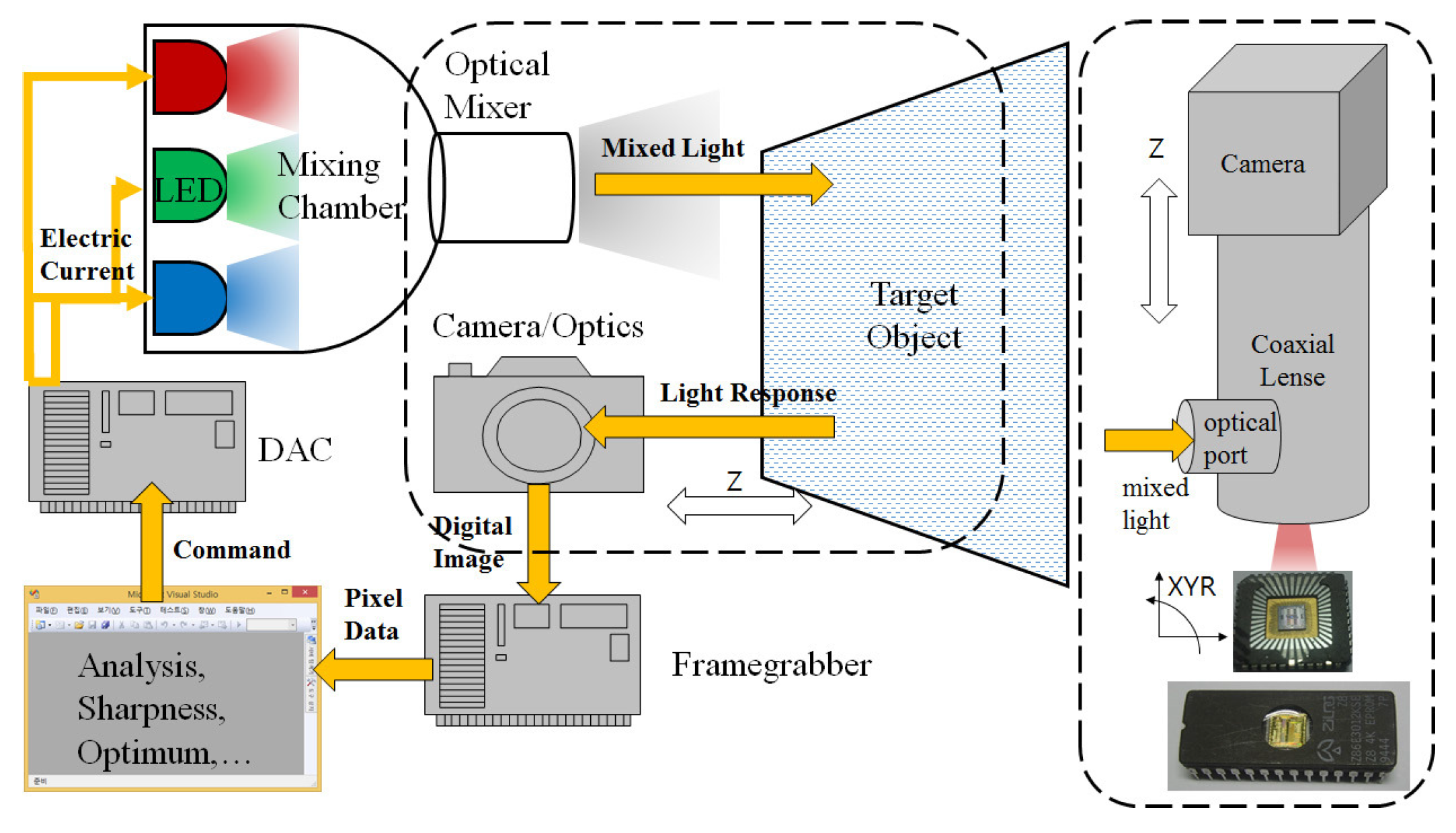
The conventional inspection system for color lighting comprises a mixed light source, industrial camera, framegrabber, controller, and light control board. Figure 1 shows a conceptual diagram of the color mixer and machine vision system. The color mixer generates a mixed light and emits it toward a target object, and the camera acquires a digital image, which is a type of response to the mixed light. The digital image is analyzed to study the image properties (e.g., image quality) and to determine the intensity levels of the LEDs in the color mixer. The intensity levels are converted into voltage level using a digital-to-analog converter (DAC) board. The electric current to drive the LEDs is generated using a current driver according to the voltage level. The color mixer and the machine vision form a feedback loop.
The image quality must be evaluated to use optimum methods. There are various image indices proposed in many papers; these are evaluated using pixel operations [23,24]. For instance, the brightness, , is calculated from the conception of the average grey level of an pixel image.
where the grey level of pixels is and the size of the image is .
Image quality is one of the image indices, and is usually estimated using sharpness. Sharpness actually indicates the deviation and difference of grey levels among pixels. There are dozens of definitions for sharpness, and standard deviation is widely used as sharpness in machine vision [25]. Thus, sharpness can be written as follows.
Industrial machine vision usually functions in a dark room so that the image acquired by a camera completely depends on the lighting system. The color mixer employed in this study uses multiple color LEDs having individual electric inputs. Because the inputs are all adjusted using the voltage level, the color mixer has a voltage input vector for N LEDs as follows.
As presented in section I, the relationship between the LED inputs and the image quality involve electric, spectral, and optical responses. This procedure cannot easily be described using a mathematical model, and the relationship from (1) to (3) is a black box function which can be denoted as an arbitrary function f, which is a cost function in this study.
The best sharpness can be obtained by adjusting V. However, V is an unknown vector. The maximum sharpness can be found using optimum methods, but negative sharpness must be defined because optimum methods are designed for finding the minimum. Hence, negative sharpness is a cost function.
The optimum methods have a general form of problem definition using a cost function as follows [17]:
2.2. Derivative Optimum Methods
The steepest descent and conjugate gradient methods are representative of the derivative optimum methods, which involve the differential operation of a cost function written as a gradient.
The STD iterates the equations until it finds a local minimum; a symbol k is necessary to show the current iteration. The STD updates current inputs by adding a negative gradient to the current inputs. is originally determined at in STD [18], however it is difficult to obtain using an experimental apparatus. In this study, the is assumed to be a constant, .
The CJG has the same method of updating the current inputs. However, the difference lies in calculating the index of the updates .
usually has an unpredictably large or small value, which causes divergence or oscillation near the optimum. Consequently, the following boundary conditions are given before updating the current inputs.
where is the convergence coefficient for a limited range and is the threshold. The updating of inputs and the acquisition of sharpness are iterated until the gradient becomes smaller than the terminal condition , which indicates that auto-lighting finds the maximum sharpness and the best image quality.
where is an infinitesimal value for the terminal condition.
The cost function is acquired using hardware, and the terminal condition considers differential values. The values are discrete and sensitive to noises; hence, an additional terminal condition, , is applied as follows:
3. Robust Parameter Design
3.1. System for Experiment
The sharpness and derivative methods were applied to a test system which was constructed in our previous study [6]. The test system was composed of a 4 M pixel camera (SVS-4021, SVS-VISTEK, Seefeld, Germany), a coaxial lens (COAX, Edmund Optics, Barrington, NJ, USA), a framegrabber (SOL6M, Matrox, Dorval, QC, Canada), a multi-channel DAC board (NI-6722, NI, Austin, TX, USA), and an RGB mixing light source. Commercial integrated circuits (ICs) of EPROMs were used as sample targets A (EP910JC35, ALTERA, San Jose, CA, USA) and B (Z86E3012KSES, ZILOG, Milpitas, CA, USA), as shown in Figure 2. The camera and the ICs were fixed on Z and XYR axes, respectively. The coaxial lens was attached to the camera, and faced the ICs. Optical fiber from the RGB source was connected to the coaxial lens and illuminated the ICs. Images of the ICs were acquired and transferred into a PC through a CAMERALINK port on the framegrabber. Operating software was constructed using a development tool (Visual Studio 2008, Microsoft, Redmond, WA, USA) and vision library (MIL 8.0, Matrox, Dorval, QC, Canada). Location of the ICs in an image was adjusted using XYR axes after focusing was performed using the Z axis. The inputs of the RGB source were connected to the DAC board. The light color and intensity were adjusted through the board. The STD and CJG for optimum light condition were implemented into the software.
3.2. Taguchi Method
The Taguchi method is commonly used to tune the algorithm parameters and optical design in machine vision [26,27,28]. A neural network is a massive and complex numerical model, and derivative optimal methods are frequently applied to its training parameters [29,30]. Taguchi method is useful to find the learning parameters of neural network and increase learning efficiency in machine vision system [31]. Considering the non-linear, multi-dimensional, and black box function systems in this study, we expected that the Taguchi method could be useful in tuning the auto-lighting algorithm. The performance of the algorithm was largely evaluated using the minimum number of iterations and the maximum sharpness. Hence, “the smaller the better” concept was applied in case of the number of iterations and “the larger the better” concept was applied in the case of the sharpness while calculating the signal-to-noise (SN) ratio. Those SN ratios can be obtained using the following equations [32,33]:
where is the performance index (e.g., sharpness and iteration), and w is the number of experiments.
3.3. Experiment Design
The selected parameters were initial voltages of red, green, and blue (RGB) LEDs, , the convergence constant , and the threshold . Because the maximum sharpness is usually formed in low-voltage regions under a single-light condition, the range of the initial voltage was less than half of the full voltage. The ranges of and were between 0.0 and 1.0. These five factors were chosen as control factors. Because all the ranges are divided into five intervals, the level was set at 5. Therefore, the model is organized using five control factors and five levels, as shown in Table 1. The combination of the experiment is 25, which is quite a small value considering the multiple color sources and the algorithm parameters. Two sample targets were used for the experiments, as proposed.
4. Results
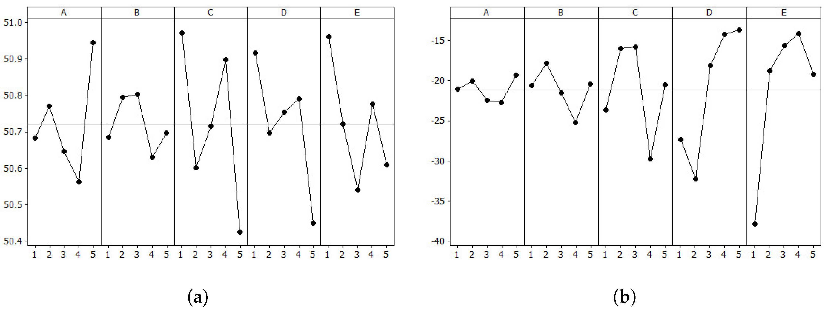
The maximum sharpness found using the ESS was at for Pattern A, and at for Pattern B. The total step number of combinations for RGB was . The orthogonal arrays for steepest descent and conjugate gradient methods were constructed as shown in Table 2 and Table 3. , , , and were the optimal statuses found by the steepest descent method by using the selected parameters. Some combinations showed almost the same sharpness as that of the exact solution, some combinations reached the maximum after several steps, and some cases failed to converge. These facts show that parameter selection for a derivative optimum is important because of stability. The SN ratios were calculated using MINITAB for mathematical operations of Taguchi analysis. Figure 3, Figure 4, Figure 5 and Figure 6 are the results of Taguchi analysis and show the trend of the control factors. The variation in the sharpness was very small, whereas the variation in the number of the iteration was larger, which implied that the parameters were sensitive to iteration.
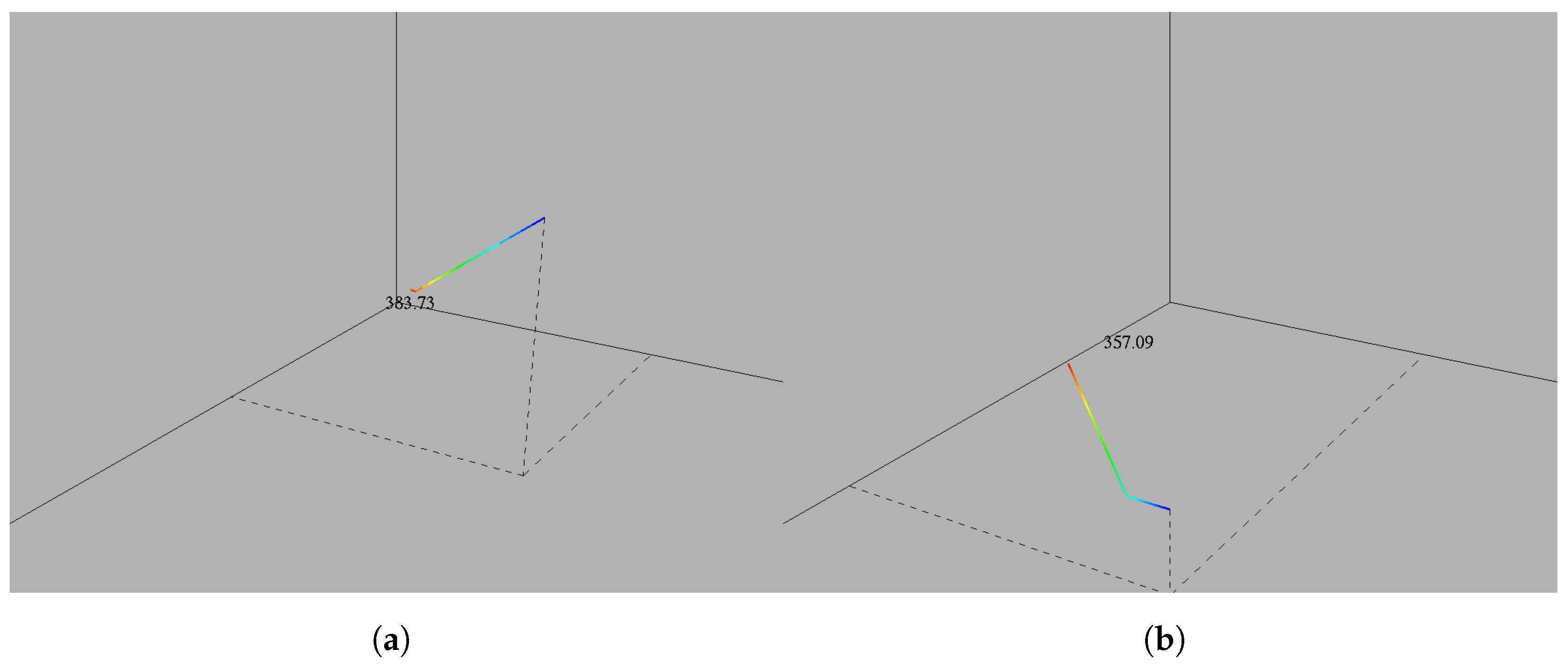
However, the trends of sharpness and the number of iterations were inverse. Sharpness is more important than the number of iterations because the inspection in a manufacturing process must be accurate. Hence, we chose the initial voltage in the sharpness, and and in the number of the iteration. Retest combinations of STD were determined considering figures such as and for Patterns A and B, respectively. , and were selected for Patterns A and B in case of CJG. The retest results using were , V = (0.00, 0.00, 1.09), and 19 iterations. The combination of was , V = (1.02, 0.00, 0.00), and 37 iterations. The retest results using were , V = (0.31, 0.30, 0.3), and 16 iterations. The value of this point was 2% lower than the ESS, and the coordinate is far from the ESS. This indicates a different local minimum compared with the ESS results. However, when the terminal condition is tightly given, a result similar to the ESS can be obtained with 74 iterations. The retest results using were , V = (1.02, 0.02, 0.00), and 37 iterations. Contributions of the parameters in the STD were evaluated using ANOVA, as shown in Table 4 and Table 5. The results of ANOVA were obtained using general linear model in MINITAB. The was the most significant factor for Pattern A, but initial point was significant for Pattern B. Table 6 and Table 7 show contributions of the parameters in the CJD. was the most significant factor for the sharpness and the iteration. However, initial point was significant for the sharpness, and the iteration was more significant for the iteration. Hence, convergence constant, , is the most important and the initial point is the second to find optimum of color lighting. was a minor factor in the experiments.
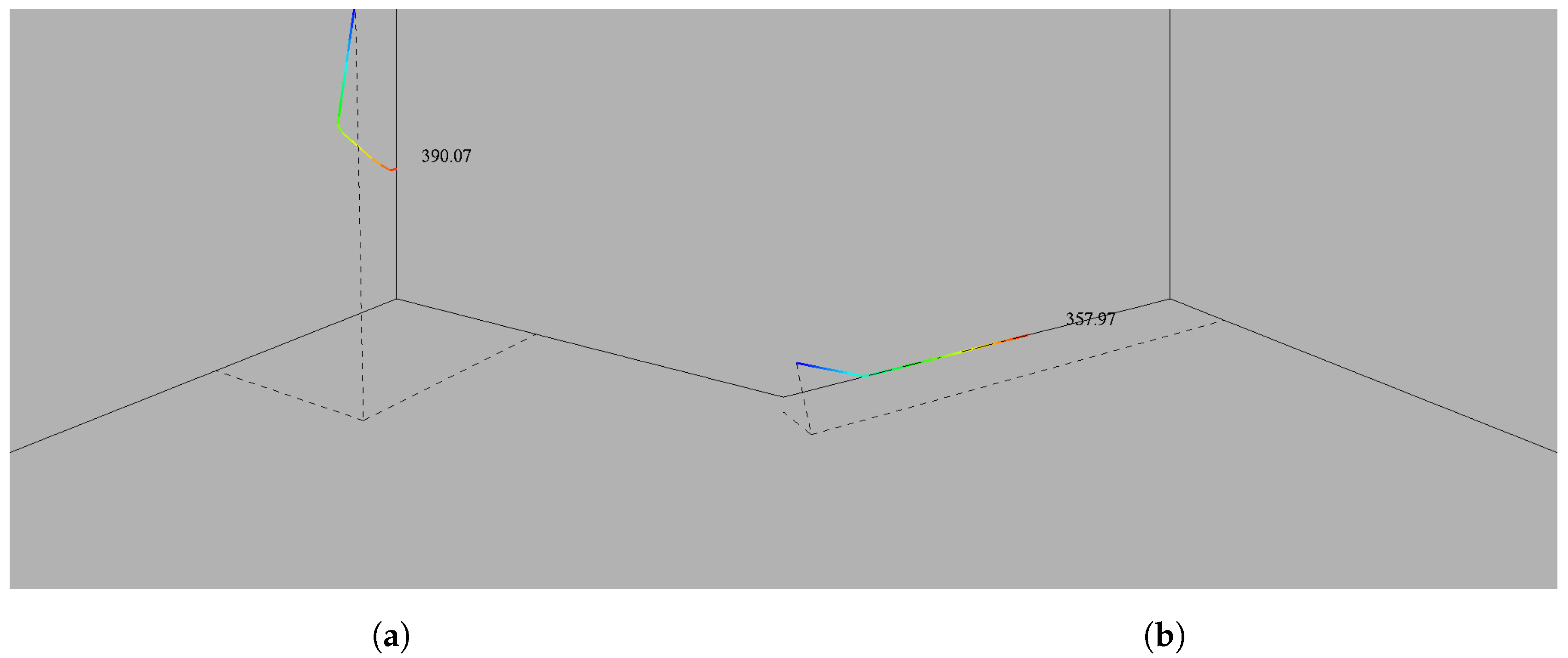
Figure 7 and Figure 8 show the convergence of maximum sharpness by employing the STD and the CJD methods. In the figures, , , and are mapped virtually in Cartesian coordinates. The starting point is shown in blue, and the color is varied into others during iteration. The terminal point is marked with red. The paths shaped smooth curve lines compared to direct and non-differentiation optimum search methods showing discrete pattern. The starting points of individual pattern determined using Taguchi method were different, but they approached the same point.
The sharpnesses in the results were almost the same as that observed in the best-case parameters. However, the number of iterations was relatively small compared to the average number of iterations—even the numbers using ESS. One result had almost the same sharpnesses as that of the exact solution using different voltage. The retest results show that the Taguchi method provides useful parameters with a small number of experiments. Although the maximum sharpness value determined by the proposed methods was a little lower than that determined by ESS, the number of iterations was much smaller. Therefore, the proposed auto-lighting algorithm can reduce the number of iterations, while the image quality remains almost the same. Furthermore, the Taguchi method can reduce laborious tasks and the setup time for the inspection process in manufacturing.
5. Conclusions
A tuning method was proposed for the auto-lighting algorithm using the Taguchi method. The algorithm maximizes the image quality by adjusting multiple light sources in the shortest time, thus providing a function called auto-lighting. The image quality is defined as sharpness—the standard deviation of the grey level in pixels of an inspected image. The best image quality was found using two differential optimum methods—STD and CJG. The image quality was represented using sharpness, and the minimum of the negative sharpness was found using the steepest descent and conjugate gradient methods. These methods are modified for auto-lighting algorithms.
The Taguchi method was applied to determine the algorithm parameters, such as initial voltage, convergence constant, and threshold. The orthogonal array was constructed considering five control factors and five levels of the parameter ranges. The SN ratio of the sharpness was calculated using “the larger the better”, and that of the number of iterations was calculated using “the smaller the better”. The desired combinations were determined after the Taguchi analysis using the orthogonal array. A retest was conducted by using the desired combination, and the results showed that the Taguchi method provides useful parameter values, and the performance is almost equal to that of the best-case parameters. The Taguchi method will be useful in reducing tasks and the time required to set up the inspection process in manufacturing.
Acknowledgments
We would like to acknowledge the financial support from the R & D Program of MOTIE (Ministry of Trade, Industry and Energy) and KEIT (Korea Evaluation Institute of Industrial Technology) of Republic of Korea (Development of Vision Block supporting the combined type I/O of extensible and flexible structure, 10063314). The authors are grateful to AM Technology (http://www.amtechnology.co.kr) for supplying RGB mixable color sources.
Author Contributions
All of the authors contributed extensively to this work presented in the paper. HyungTae Kim conceived the optimum algorithm, conducted the experiments and wrote the paper. KyeongYong Cho conducted the experiment using the Taguchi method. KyungChan Jin designed the experimental apparatus and Jongseok Kim constructed the apparatus. SeungTaek Kim derived color coordinates and analyzed the data.
Conflicts of Interest
The authors declare no conflict of interest.
Abbreviations
| STD | Steepest descent method |
| CJG | Conjugate gradient method |
| LED | Light emitting diode |
| RGB | Red, green and blue |
| sRGB | Standard red, green and blue |
| ESS | Equal step search |
| TAE | Trial-and-error |
| SN | Signal-to-noise |
| Grey level of an image pixel | |
| Brightness, average grey level of an image | |
| k | Current iteration |
| m | Horizontal pixel number of an image |
| N | Number of voltage inputs for a color mixer |
| n | Vertical pixel number of an image |
| u | the performance index |
| V | Vector of voltage inputs for a color mixer |
| v | Individual voltage input for an LED |
| w | the number of experiments |
| x | Horizontal coordinate of an image |
| y | Vertical coordinate of an image |
| Convergence coefficient | |
| Terminal condition | |
| Convergence coefficient for limited range | |
| Negative sharpness, cost function | |
| Sharpness, image quality | |
| Threshold | |
| Index of update for conjugate gradient method |
References
- Gruber, F.; Wollmann, P.; Schumm, B.; Grahlert, W.; Kaskel, S. Quality Control of Slot-Die Coated Aluminum Oxide Layers for Battery Applications Using Hyperspectral Imaging. J. Imaging 2016, 2, 12. [Google Scholar] [CrossRef]
- Neogi, N.; Mohanta, D.K.; Dutta, P.K. Review of vision-based steel surface inspection systems. EURASIP J. Image Video Process. 2014, 50, 1–19. [Google Scholar] [CrossRef]
- Arecchi, A.V.; Messadi, T.; Koshel, R.J. Field Guide to Illimination; SPIE Press: Bellingham, WA, USA, 2007; pp. 110–115. [Google Scholar]
- Pfeifer, T.; Wiegers, L. Reliable tool wear monitoring by optimized image and illumination control in machine vision. Measurement 2010, 28, 209–218. [Google Scholar] [CrossRef]
- Jani, U.; Reijo, T. Setting up task-optimal illumination automatically for inspection purposes. Proc. SPIE 2007, 6503, 65030K. [Google Scholar]
- Kim, T.H.; Kim, S.T.; Cho, Y.J. Quick and Efficient Light Control for Conventional AOI Systems. Int. J. Precis. Eng. Manuf. 2015, 16, 247–254. [Google Scholar] [CrossRef]
- Chen, S.Y.; Zhang, J.W.; Zhang, H.X.; Kwok, N.M.; Li, Y.F. Intelligent Lighting Control for Vision-Based Robotic Manipulation. IEEE Trans. Ind. Electron. 2012, 59, 3254–3263. [Google Scholar] [CrossRef]
- Victoriano, P.M.A.; Amaral, T.G.; Dias, O.P. Automatic Optical Inspection for Surface Mounting Devices with IPC-A-610D compliance. In Proceedings of the 2011 International Conference on Power Engineering, Energy and Electrical Drives (POWERENG), Malaga, Spain, 11–13 May 2011; pp. 1–7. [Google Scholar]
- Muthu, S.; Gaines, J. Red, Green and Blue LED-based White Light Source: Implementation Challenges and Control Design. In Proceedings of the 2003 38th IAS Annual Meeting, Conference Record of the Industry Applications Conference, Salt Lake City, UT, USA, 12–16 October 2003; Volume 1, pp. 515–522. [Google Scholar]
- Esparza, D.; Moreno, I. Color patterns in a tapered lightpipe with RGB LEDs. Proc. SPIE 2010, 7786, 77860I. [Google Scholar]
- Van Gorkom, R.P.; van AS, M.A.; Verbeek, G.M.; Hoelen, C.G.A.; Alferink, R.G.; Mutsaers, C.A.; Cooijmans, H. Etendue conserved color mixing. Proc. SPIE 2007, 6670, 66700E. [Google Scholar]
- Zhu, Z.M.; Qu, X.H.; Liang, H.Y.; Jia, G.X. Effect of color illumination on color contrast in color vision application. Proc. SPIE Opt. Metrol. Insp. Ind. Appl. 2010, 7855, 785510. [Google Scholar]
- Park, J.I.; Lee, M.H.; Grossberg, M.D.; Nayar, S.K. Multispectral Imaging Using Multiplexed Illumination. In Proceedings of the IEEE 11th International Conference on Computer Vision (ICCV 2007), Rio de Janeiro, Brazil, 14–20 October 2007; pp. 1–8. [Google Scholar]
- Lee, M.H.; Seo, D.K.; Seo, B.K.; Park, J.I. Optimal Illumination Spectrum for Endoscope. In Proceedings of the 2011 17th Korea-Japan Joint Workshop on Frontiers of Computer Vision (FCV), Ulsan, Korea, 9–11 February 2011; pp. 1–6. [Google Scholar]
- Kim, T.H.; Kim, S.T.; Cho, Y.J. An Optical Mixer and RGB Control for Fine Images using Grey Scale Distribution. Int. J. Optomech. 2012, 6, 213–225. [Google Scholar] [CrossRef]
- Kim, T.H.; Kim, S.T.; Kim, J.S. Mixed-color illumination and quick optimum search for machine vision. Int. J. Optomech. 2013, 7, 208–222. [Google Scholar] [CrossRef]
- Kim, T.H.; Cho, K.Y.; Jin, K.C.; Yoon, J.S.; Cho, Y.J. Mixing and Simplex Search for Optimal Illumination in Machine Vision. Int. J. Optomech. 2014, 8, 206–217. [Google Scholar] [CrossRef]
- Arora, J.S. Introduction to Optimum Design, 2nd ed.; Academic Press: San Diego, CA, USA, 2004; pp. 433–465. [Google Scholar]
- Kim, T.H.; Cho, K.Y.; Kim, S.T.; Kim, J.S.; Jin, K.C.; Lee, S.H. Rapid Automatic Lighting Control of a Mixed Light Source for Image Acquisition using Derivative Optimum Search Methods. In Proceedings of the International Symposium of Optomechatronics Technology (ISOT 2015), Neuchâtel, Switzerland, 14–16 October 2015; p. 07004. [Google Scholar]
- Dey, N.; Ashour, A.S.; Beagum, S.; Pistola, D.S.; Gospodinov, M.; Gospodinova, E.P.; Tavares, J.M.R.S. Parameter Optimization for Local Polynomial Approximation based Intersection Confidence Interval Filter Using Genetic Algorithm: An Application for Brain MRI Image De-Noising. J. Imaging 2015, 1, 60–84. [Google Scholar] [CrossRef]
- Lazarevic, D.; Madic, M.; Jankovic, P.; Lazarevic, A. Cutting Parameters Optimization for Surface Roughness in Turning Operation of Polyethylene (PE) Using Taguchi Method. Tribol. Ind. 2012, 34, 68–73. [Google Scholar]
- Verma, J.; Agrawal, P.; Bajpai, L. Turning Parameter Optimization for Surface Roughness of Astm A242 Type-1 Alloys Steel by Taguchi Method. Int. J. Adv. Eng. Technol. 2012, 3, 255–261. [Google Scholar]
- Firestone, L.; Cook, K.; Culp, K.; Talsania, N.; Preston, K., Jr. Comparision of Autofocus Methods for Automated Microscopy. Cytometry 1991, 12, 195–206. [Google Scholar] [CrossRef] [PubMed]
- Bueno-Ibarra, M.A.; Alvarez-Borrego, J.; Acho, L.; Chavez-Sanchez, M.C. Fast autofocus algorithm for automated microscopes. Opt. Eng. 2005, 44, 063601. [Google Scholar]
- Sun, Y.; Duthaler, S.; Nelson, B.J. Autofocusing in computer microscopy: Selecting the optimal focus algorithm. Microsc. Res. Tech. 2004, 65, 139–149. [Google Scholar] [CrossRef] [PubMed]
- Muruganantham, C.; Jawahar, N.; Ramamoorthy, B.; Giridhar, D. Optimal settings for vision camera calibration. Int. J. Manuf. Technol. 2010, 42, 736–748. [Google Scholar] [CrossRef]
- Li, M.; Milor, L.; Yu, W. Developement of Optimum Annular Illumination: A Lithography-TCAD Approach. In Proceedings of the Advanced Semiconductor Manufacturing Conference and Workshop (IEEE/SEMI ), Cambridge, MA, USA, 10–12 September 1997; pp. 317–321. [Google Scholar]
- Kim, T.H.; Cho, K.Y.; Kim, S.T.; Kim, J.S. Optimal RGB Light-Mixing for Image Acquisition Using Random Search and Robust Parameter Design. In Proceedings of the 16th International Workshop on Combinatorial Image Analysis, Brno, Czech Republic, 28–30 May 2014; Volume 8466, pp. 171–185. [Google Scholar]
- Zahlay, F.D.; Rao, K.S.R.; Baloch, T.M. Autoreclosure in Extra High Voltage Lines using Taguchi’s Method and Optimized Neural Network. In Proceedings of the 2008 Electric Power Conference (EPEC), Vancouver, BC, Canada, 6–7 October 2008; Volume 2, pp. 151–155. [Google Scholar]
- Sugiono; Wu, M.H.; Oraifige, I. Employ the Taguchi Method to Optimize BPNN’s Architectures in Car Body Design System. Am. J. Comput. Appl. Math. 2012, 2, 140–151. [Google Scholar]
- Su, T.L.; Chen, H.W.; Hong, G.B.; Ma, C.M. Automatic Inspection System for Defects Classification of Stretch Kintted Fabrics. In Proceedings of the 2010 International Conference on Wavelet Analysis and Pattern Recognition (ICWAPR), Qingdao, China, 11–14 July 2010; pp. 125–129. [Google Scholar]
- Wu, Y.; Wu, A. Quality engineering and experimental design. In Taguchi Methods for Robust Design; The American Society of Mechanical Engineers: Fairfield, NJ, USA, 2000; pp. 3–16. [Google Scholar]
- Yoo, W.S.; Jin, Q.Q.; Chung, Y.B. A Study on the Optimization for the Blasting Process of Glass by Taguchi Method. J. Soc. Korea Ind. Syst. Eng. 2007, 30, 8–14. [Google Scholar]
Figure 1.
System Diagram for color mixing and automatic lighting.

Figure 2.
Target patterns acquired by maximum sharpness: (a) Pattern A; (b) Pattern B.
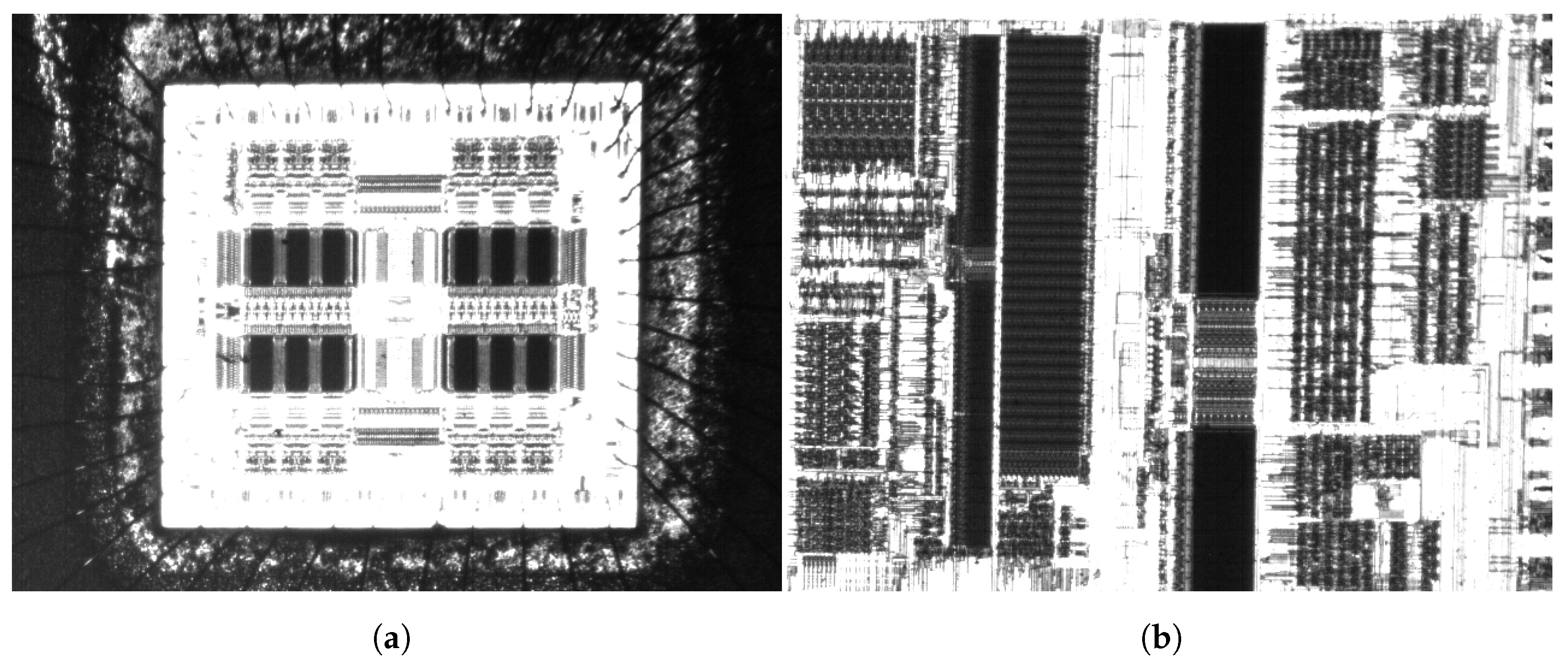
Figure 3.
Signal-to-noise (SN) ratios of control factors for Pattern A in the case of steepest descent method: (a) Sharpness; (b) Iterations.
Figure 3.
Signal-to-noise (SN) ratios of control factors for Pattern A in the case of steepest descent method: (a) Sharpness; (b) Iterations.
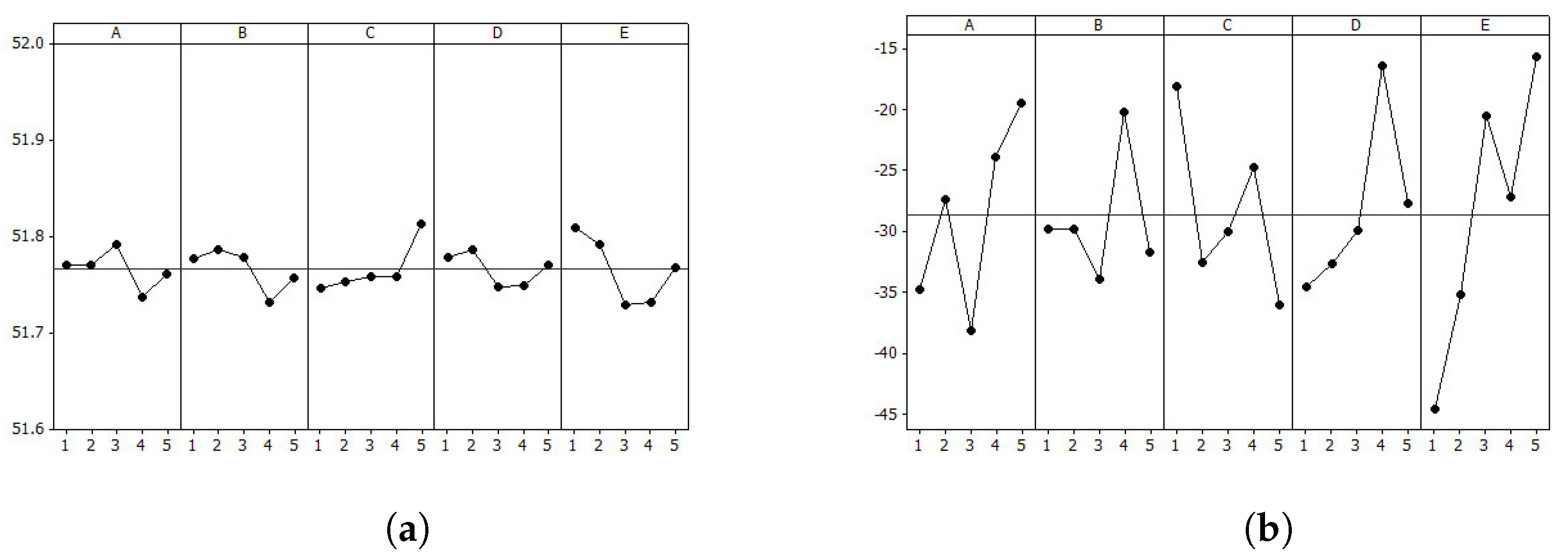
Figure 4.
SN ratios of control factors for Pattern B in the case of steepest descent method: (a) Sharpness; (b) Iterations.
Figure 4.
SN ratios of control factors for Pattern B in the case of steepest descent method: (a) Sharpness; (b) Iterations.

Figure 5.
SN ratios of control factors for Pattern A in the case of conjugate gradient method: (a) Sharpness; (b) Iterations.
Figure 5.
SN ratios of control factors for Pattern A in the case of conjugate gradient method: (a) Sharpness; (b) Iterations.
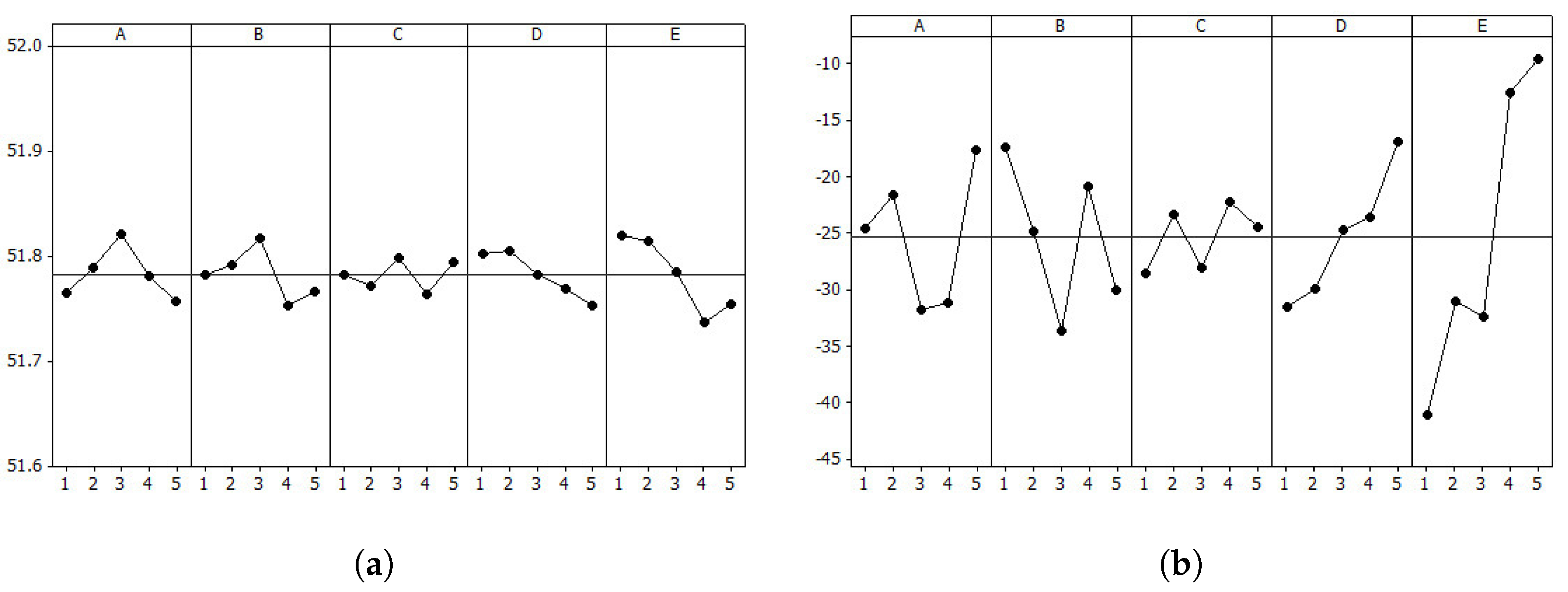
Figure 6.
SN ratios of control factors for Pattern B in the case of conjugate gradient method: (a) Sharpness; (b) Iterations.
Figure 6.
SN ratios of control factors for Pattern B in the case of conjugate gradient method: (a) Sharpness; (b) Iterations.

Figure 7.
Search path formed by steepest descent method using Patterns (a) A and (b) B.

Figure 8.
Search path formed by conjugate gradient method using Patterns (a) A and (b) B.

Table 1.
Control factors and levels for derivative optimum methods.
| Factors | Code | Level | ||||
|---|---|---|---|---|---|---|
| 1 | 2 | 3 | 4 | 5 | ||
| : Initial | A | 0.5 | 1.0 | 1.5 | 2.0 | 2.5 |
| : Initial | B | 0.5 | 1.0 | 1.5 | 2.0 | 2.5 |
| : Initial | C | 0.5 | 1.0 | 1.5 | 2.0 | 2.5 |
| : Threshold | D | 0.2 | 0.4 | 0.6 | 0.8 | 1.0 |
| : Convergence Constant | E | 0.2 | 0.4 | 0.6 | 0.8 | 1.0 |
Table 2.
Orthogonal array of steepest descent method for Patterns A and B.
| Run # | Control Factors | Pattern A | Pattern B | ||||||||||||
|---|---|---|---|---|---|---|---|---|---|---|---|---|---|---|---|
| A | B | C | D | E | |||||||||||
| 1 | 1 | 1 | 1 | 1 | 1 | 389.43 | 117 | 0.98 | 0.00 | 0.41 | 353.88 | 153 | 0.53 | 0.30 | 0.00 |
| 2 | 1 | 2 | 2 | 2 | 2 | 390.50 | 255 | 0.00 | 0.00 | 1.25 | - | - | - | - | - |
| 3 | 1 | 3 | 3 | 3 | 3 | - | - | - | - | - | 340.47 | 3 | 0.00 | 0.42 | 0.42 |
| 4 | 1 | 4 | 4 | 4 | 4 | 382.4 | 2 | 0.00 | 0.72 | 0.72 | - | - | - | - | - |
| 5 | 1 | 5 | 5 | 5 | 5 | 390.43 | 152 | 0.00 | 0.00 | 1.30 | 317.63 | 2 | 0.00 | 0.53 | 0.82 |
| 6 | 2 | 1 | 2 | 3 | 4 | 386.09 | 189 | 0.52 | 0.02 | 0.52 | 344.02 | 1 | 0.52 | 0.02 | 0.52 |
| 7 | 2 | 2 | 3 | 4 | 5 | 387.22 | 1 | 0.20 | 0.20 | 0.70 | 337.22 | 1 | 0.20 | 0.20 | 0.70 |
| 8 | 2 | 3 | 4 | 5 | 1 | 390.40 | 123 | 0.00 | 0.00 | 1.26 | 333.35 | 6 | 0.00 | 0.30 | 0.80 |
| 9 | 2 | 4 | 5 | 1 | 2 | 390.36 | 49 | 0.00 | 0.00 | 1.27 | 335.65 | 22 | 0.00 | 0.24 | 0.74 |
| 10 | 2 | 5 | 1 | 2 | 3 | 384.64 | 6 | 0.00 | 1.06 | 0.00 | 346.93 | 108 | 0.00 | 0.58 | 0.00 |
| 11 | 3 | 1 | 3 | 5 | 2 | 389.01 | 109 | 0.75 | 0.02 | 0.57 | - | - | - | - | - |
| 12 | 3 | 2 | 4 | 1 | 3 | 388.87 | 263 | 0.78 | 0.00 | 0.51 | 340.46 | 11 | 0.42 | 0.00 | 0.68 |
| 13 | 3 | 3 | 5 | 2 | 4 | 390.36 | 164 | 0.00 | 0.00 | 1.29 | 324.30 | 107 | 0.00 | 0.00 | 0.90 |
| 14 | 3 | 4 | 1 | 3 | 5 | 385.88 | 3 | 0.41 | 0.70 | 0.00 | 331.85 | 2 | 0.30 | 0.80 | 0.00 |
| 15 | 3 | 5 | 2 | 4 | 1 | 389.21 | 237 | 0.99 | 0.00 | 0.38 | 346.91 | 192 | 0.00 | 0.58 | 0.00 |
| 16 | 4 | 1 | 4 | 2 | 5 | 387.71 | 3 | 0.80 | 0.00 | 0.80 | 338.46 | 18 | 0.40 | 0.00 | 0.40 |
| 17 | 4 | 2 | 5 | 3 | 1 | 389.18 | 206 | 1.04 | 0.00 | 0.36 | 338.25 | 15 | 0.30 | 0.00 | 0.70 |
| 18 | 4 | 3 | 1 | 4 | 2 | - | - | - | - | - | 354.62 | 4 | 0.72 | 0.22 | 0.00 |
| 19 | 4 | 4 | 2 | 5 | 3 | 382.32 | 2 | 0.80 | 0.80 | 0.00 | 303.61 | 2 | 0.82 | 0.80 | 0.00 |
| 20 | 4 | 5 | 3 | 1 | 4 | 384.95 | 49 | 0.24 | 0.74 | 0.00 | 349.91 | 151 | 0.24 | 0.42 | 0.00 |
| 21 | 5 | 1 | 5 | 4 | 3 | 387.90 | 4 | 0.58 | 0.00 | 0.60 | 341.62 | 4 | 0.58 | 0.00 | 0.58 |
| 22 | 5 | 2 | 1 | 5 | 4 | 386.36 | 2 | 1.28 | 0.00 | 0.00 | 358.14 | 2 | 0.90 | 0.00 | 0.00 |
| 23 | 5 | 3 | 2 | 1 | 5 | 386.78 | 6 | 1.30 | 0.30 | 0.00 | 358.26 | 82 | 0.90 | 0.00 | 0.00 |
| 24 | 5 | 4 | 3 | 2 | 1 | 389.05 | 191 | 1.08 | 0.00 | 0.32 | 355.32 | 23 | 0.66 | 0.16 | 0.00 |
| 25 | 5 | 5 | 4 | 3 | 2 | 386.50 | 8 | 0.58 | 0.58 | 0.08 | 350.51 | 137 | 0.34 | 0.34 | 0.00 |
Table 3.
Orthogonal array of conjugate gradient method for Patterns A and B.
| Run # | Control Factors | Pattern A | Pattern B | ||||||||||||
|---|---|---|---|---|---|---|---|---|---|---|---|---|---|---|---|
| A | B | C | D | E | |||||||||||
| 1 | 1 | 1 | 1 | 1 | 1 | 389.28 | 59 | 0.99 | 0.00 | 0.43 | 358.49 | 143 | 0.95 | 0.00 | 0.00 |
| 2 | 1 | 2 | 2 | 2 | 2 | 390.58 | 41 | 0.00 | 0.00 | 1.25 | 343.00 | 24 | 0.48 | 0.16 | 0.43 |
| 3 | 1 | 3 | 3 | 3 | 3 | 390.43 | 139 | 0.00 | 0.00 | 1.20 | 340.21 | 3 | 0.00 | 0.42 | 0.42 |
| 4 | 1 | 4 | 4 | 4 | 4 | 382.42 | 2 | 0.00 | 0.72 | 0.72 | 354.05 | 9 | 0.80 | 0.00 | 0.00 |
| 5 | 1 | 5 | 5 | 5 | 5 | 384.66 | 2 | 0.00 | 0.57 | 0.78 | 316.46 | 2 | 0.00 | 0.50 | 0.88 |
| 6 | 2 | 1 | 2 | 3 | 4 | 386.07 | 1 | 0.52 | 0.02 | 0.52 | 343.92 | 1 | 0.52 | 0.02 | 0.52 |
| 7 | 2 | 2 | 3 | 4 | 5 | 387.16 | 1 | 0.20 | 0.20 | 0.70 | 337.14 | 1 | 0.20 | 0.20 | 0.70 |
| 8 | 2 | 3 | 4 | 5 | 1 | 390.40 | 50 | 0.00 | 0.00 | 1.30 | 358.43 | 168 | 0.98 | 0.00 | 0.00 |
| 9 | 2 | 4 | 5 | 1 | 2 | 390.54 | 28 | 0.00 | 0.00 | 1.27 | 338.89 | 29 | 0.24 | 0.16 | 0.66 |
| 10 | 2 | 5 | 1 | 2 | 3 | 388.64 | 178 | 0.74 | 0.02 | 0.71 | 350.01 | 21 | 0.48 | 0.41 | 0.00 |
| 11 | 3 | 1 | 3 | 5 | 2 | 390.42 | 24 | 0.00 | 0.00 | 1.28 | 331.95 | 2 | 0.70 | 0.00 | 0.70 |
| 12 | 3 | 2 | 4 | 1 | 3 | 390.50 | 144 | 0.00 | 0.00 | 1.25 | 352.28 | 16 | 0.58 | 0.24 | 0.08 |
| 13 | 3 | 3 | 5 | 2 | 4 | 390.37 | 17 | 0.00 | 0.00 | 1.31 | 324.42 | 15 | 0.00 | 0.00 | 0.90 |
| 14 | 3 | 4 | 1 | 3 | 5 | 388.16 | 5 | 1.48 | 0.00 | 0.00 | 347.42 | 33 | 0.00 | 0.60 | 0.00 |
| 15 | 3 | 5 | 2 | 4 | 1 | 390.39 | 284 | 0.00 | 0.00 | 1.29 | 348.20 | 26 | 0.11 | 0.63 | 0.00 |
| 16 | 4 | 1 | 4 | 2 | 5 | 387.61 | 3 | 0.80 | 0.00 | 0.80 | 338.48 | 124 | 0.40 | 0.00 | 0.40 |
| 17 | 4 | 2 | 5 | 3 | 1 | 390.43 | 273 | 0.00 | 0.00 | 1.24 | 342.81 | 38 | 0.28 | 0.28 | 0.43 |
| 18 | 4 | 3 | 1 | 4 | 2 | 390.43 | 264 | 0.00 | 0.00 | 1.25 | 354.42 | 4 | 0.72 | 0.22 | 0.00 |
| 19 | 4 | 4 | 2 | 5 | 3 | 387.57 | 7 | 0.95 | 0.60 | 0.00 | 304.10 | 2 | 0.80 | 0.80 | 0.00 |
| 20 | 4 | 5 | 3 | 1 | 4 | 387.84 | 39 | .00 | 0.27 | 0.91 | 349.67 | 13 | 0.24 | 0.42 | 0.00 |
| 21 | 5 | 1 | 5 | 4 | 3 | 387.92 | 5 | 0.74 | 0.08 | 0.70 | 338.57 | 4 | 0.58 | 0.00 | 0.65 |
| 22 | 5 | 2 | 1 | 5 | 4 | 384.69 | 1 | 1.70 | 0.20 | 0.00 | 358.02 | 2 | 0.90 | 0.00 | 0.00 |
| 23 | 5 | 3 | 2 | 1 | 5 | 387.46 | 8 | 0.90 | 0.30 | 0.20 | 357.96 | 8 | 0.90 | 0.00 | 0.00 |
| 24 | 5 | 4 | 3 | 2 | 1 | 389.12 | 80 | 0.93 | 0.00 | 0.42 | 358.45 | 118 | 0.95 | 0.00 | 0.00 |
| 25 | 5 | 5 | 4 | 3 | 2 | 386.35 | 8 | 0.58 | 0.58 | 0.08 | 350.36 | 9 | 0.34 | 0.34 | 0.00 |
Table 4.
ANOVA of Pattern A for contribution of steepest descent method.
| Control Factors | l | |||||||
|---|---|---|---|---|---|---|---|---|
| Source | Parameter | DF | SS | MS | Contribution (%) | SS | MS | Contribution (%) |
| A | Initial | 4 | 19.548 | 4.887 | 14.2 | 71,168 | 17,792 | 24.5 |
| B | Initial | 4 | 18.847 | 4.712 | 13.7 | 36,910 | 9228 | 12.7 |
| C | Initial | 4 | 34.290 | 8.572 | 23.0 | 65,697 | 16,424 | 22.6 |
| D | 4 | 17.188 | 4.297 | 12.5 | 43,406 | 10,851 | 14.9 | |
| E | 4 | 41.656 | 10.414 | 30.3 | 71,069 | 17,767 | 24.5 | |
| Error | 2 | 5.806 | 2.903 | 4.2 | 2171 | 1085 | 0.7 | |
| Total | 22 | 137.335 | 290,421 | |||||
Table 5.
ANOVA of Pattern B for contribution of steepest descent method.
| Control Factors | l | |||||||
|---|---|---|---|---|---|---|---|---|
| Source | Parameter | DF | SS | MS | Contribution (%) | SS | MS | Contribution (%) |
| A | Initial | 4 | 1094.64 | 273.66 | 24.0 | 4027 | 1007 | 4.5 |
| B | Initial | 4 | 916.54 | 229.13 | 20.1 | 40,860 | 10,215 | 45.6 |
| C | Initial | 4 | 1019.66 | 254.91 | 22.4 | 2807 | 702 | 3.1 |
| D | 4 | 715.99 | 179 | 15.7 | 17,557 | 4389 | 19.6 | |
| E | 4 | 516.07 | 129.02 | 11.3 | 10,919 | 2730 | 12.2 | |
| Error | 4 | 291.90 | 72.97 | 6.4 | 13,524 | 3381 | 15.1 | |
| Total | 24 | 4554.80 | 89,694 | |||||
Table 6.
ANOVA of Pattern A for contribution of conjugate gradient method.
| Control Factors | l | |||||||
|---|---|---|---|---|---|---|---|---|
| Source | Parameter | DF | SS | MS | Contribution (%) | SS | MS | Contribution (%) |
| A | Initial | 4 | 24.802 | 6.2 | 18.5 | 30,195 | 7549 | 14.8 |
| B | Initial | 4 | 23.749 | 5.937 | 17.7 | 34,288 | 8572 | 16.9 |
| C | Initial | 4 | 8.295 | 2.074 | 6.2 | 9756 | 2439 | 4.8 |
| D | 4 | 19.159 | 4.8 | 14.3 | 24,720 | 6180 | 12.1 | |
| E | 4 | 51.27 | 12.818 | 38.2 | 72,863 | 18,216 | 35.8 | |
| Error | 4 | 7.054 | 1.763 | 5.3 | 31,656 | 7914 | 15.6 | |
| Total | 24 | 134.329 | 203,478 | |||||
Table 7.
ANOVA of Pattern B for contribution of conjugate gradient method.
| Control Factors | l | |||||||
|---|---|---|---|---|---|---|---|---|
| Source | Parameter | DF | SS | MS | Contribution (%) | SS | MS | Contribution (%) |
| A | Initial | 4 | 637.8 | 159.5 | 14.3 | 1884.4 | 471.1 | 3.3 |
| B | Initial | 4 | 161.4 | 40.3 | 3.6 | 5903.6 | 1475.9 | 10.3 |
| C | Initial | 4 | 1491.5 | 372.9 | 33.4 | 8974.8 | 2243.7 | 15.6 |
| D | 4 | 840.4 | 210.1 | 18.8 | 8401.6 | 2100.4 | 14.6 | |
| E | 4 | 794.9 | 198.7 | 17.8 | 29,353.6 | 7338.4 | 51.1 | |
| Error | 4 | 537.4 | 134.3 | 12.0 | 2888 | 722 | 5.0 | |
| Total | 24 | 4463.4 | 57,406 | |||||
© 2017 by the authors. Licensee MDPI, Basel, Switzerland. This article is an open access article distributed under the terms and conditions of the Creative Commons Attribution (CC BY) license (http://creativecommons.org/licenses/by/4.0/).
Share and Cite
MDPI and ACS Style
Kim, H.; Cho, K.; Kim, J.; Jin, K.; Kim, S. Robust Parameter Design of Derivative Optimization Methods for Image Acquisition Using a Color Mixer. J. Imaging 2017, 3, 31. https://doi.org/10.3390/jimaging3030031
AMA Style
Kim H, Cho K, Kim J, Jin K, Kim S. Robust Parameter Design of Derivative Optimization Methods for Image Acquisition Using a Color Mixer. Journal of Imaging. 2017; 3(3):31. https://doi.org/10.3390/jimaging3030031
Chicago/Turabian StyleKim, HyungTae, KyeongYong Cho, Jongseok Kim, KyungChan Jin, and SeungTaek Kim. 2017. "Robust Parameter Design of Derivative Optimization Methods for Image Acquisition Using a Color Mixer" Journal of Imaging 3, no. 3: 31. https://doi.org/10.3390/jimaging3030031
Note that from the first issue of 2016, this journal uses article numbers instead of page numbers. See further details here.