Improving CNN-Based Texture Classification by Color Balancing


1
Department of Computer Science, Systems and Communications, University of Milano-Bicocca, 20126 Milan, Italy
2
Department of Electrical, Computer and Biomedical Engineering, University of Pavia, 27100 Pavia, Italy
*
Author to whom correspondence should be addressed.
J. Imaging 2017, 3(3), 33; https://doi.org/10.3390/jimaging3030033
Submission received: 29 June 2017
/
Revised: 17 July 2017
/
Accepted: 21 July 2017
/
Published: 27 July 2017
(This article belongs to the Special Issue Color Image Processing)
Abstract
:Texture classification has a long history in computer vision. In the last decade, the strong affirmation of deep learning techniques in general, and of convolutional neural networks (CNN) in particular, has allowed for a drastic improvement in the accuracy of texture recognition systems. However, their performance may be dampened by the fact that texture images are often characterized by color distributions that are unusual with respect to those seen by the networks during their training. In this paper we will show how suitable color balancing models allow for a significant improvement in the accuracy in recognizing textures for many CNN architectures. The feasibility of our approach is demonstrated by the experimental results obtained on the RawFooT dataset, which includes texture images acquired under several different lighting conditions.
1. Introduction
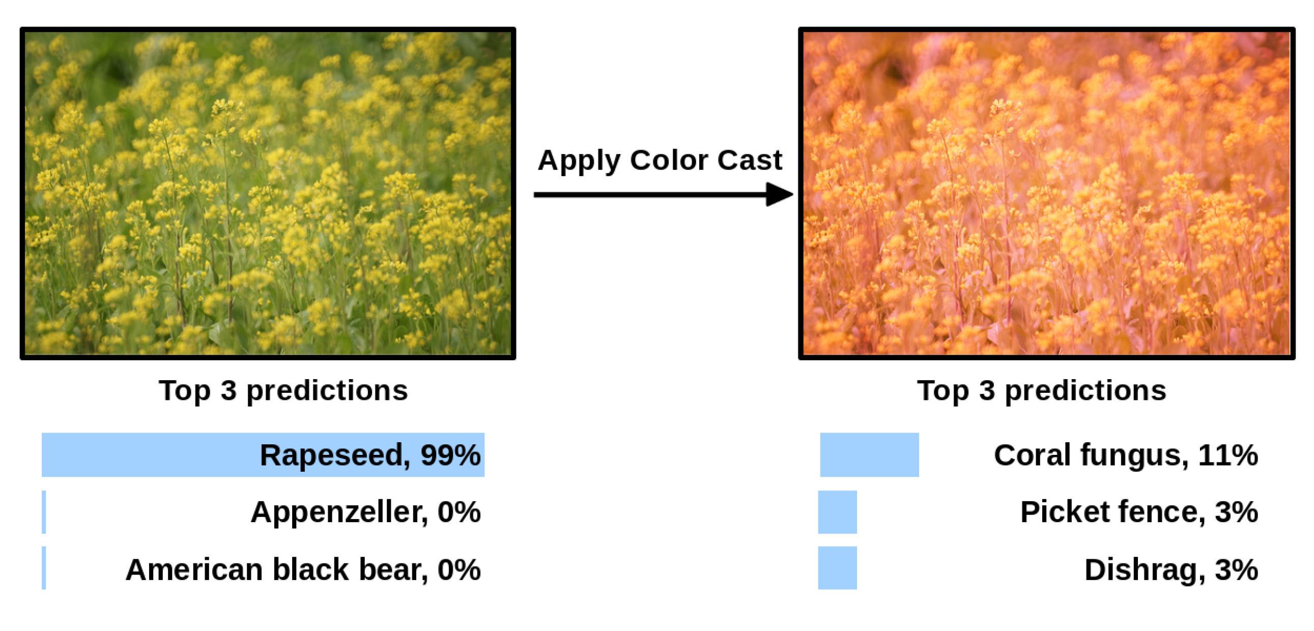
Convolutional neural networks (CNNs) represent the state of the art for many image classification problems [1,2,3]. They are trained for a specific task by exploiting a large set of images representing the application domain. During the training and the test stages, it is common practice to preprocess the input images by centering their color distribution around the mean color computed on the training set. However, when test images have been taken under acquisition conditions unseen during training, or with a different imaging device, this simple preprocessing may not be enough (see the example reported in Figure 1 and the work by Chen et al. [4]).
The most common approach to deal with variable acquisition conditions consists of applying a color constancy algorithm [5], while to obtain device-independent color description a color characterization procedure is applied [6]. A standard color-balancing model is therefore composed of two modules: the first discounts the illuminant color, while the second maps the image colors from the device-dependent RGB space into a standard device-independent color space. More effective pipelines have been proposed [7,8] that deal with the cross-talks between the two processing modules.
In this paper we systematically investigate different color-balancing models in the context of CNN-based texture classification under varying illumination conditions. To this end, we performed our experiments on the RawFooT texture database [9] which includes images of textures acquired under a large number of controlled combinations of illumination color, direction and intensity.
Concerning CNNs, when the training set is not big enough, an alternative to the full training procedure consists of adapting an already trained network to a new classification task by retraining only a small subset of parameters [10]. Another possibility is to use a pretrained network as a feature extractor for another classification method (nearest neighbor, for instance). In particular, it is common to use networks trained for the ILSVRC contest [11]. The ILSVRC training set includes over one million images taken from the web to represent 1000 different concepts. The acquisition conditions of training images are not controlled, but we may safely assume that they have been processed by digital processing pipelines that mapped them into the standard sRGB color space. We will investigate how different color-balancing models permit adapting images from the RawFooT dataset in such a way that they can be more reliably classified by several pretrained networks.
The rest of the paper is organized as follows: Section 2 summarizes the state of the art in both texture classification and color-balancing; Section 3 presents the data and the methods used in this work; Section 4 describes the experimental setup and Section 5 reports and discusses the results of the experiments. Finally, Section 6 concludes the paper by highlighting its main outcomes and by outlining some directions for future research on this topic.
2. Related Works
2.1. Color Texture Classification under Varying Illumination Conditions
Most of the research efforts on the topic of color texture classification have been devoted to the definition of suitable descriptors able to capture the distinctive properties of the texture images while being invariant, or at least robust, with respect to some variations in the acquisition conditions, such as rotations and scalings of the image, changes in brightness, contrast, light color temperature, and so on [12].
Color and texture information can be combined in several ways. Palm categorized them into parallel (i.e., separate color and texture descriptors), sequential (in which color and texture analysis are consecutive steps of the processing pipeline) and integrative (texture descriptors computed on different color planes) approaches [13]. The effectiveness of several combinations of color and texture descriptors has been assessed by Mäenpää, and Pietikäinen [14], who showed how the descriptors in the state of the art performed poorly in the case of a variable color of the illuminant. Their findings have been more recently confirmed by Cusano et al. [9].
In order to successfully exploit color in texture classification the descriptors need to be invariant (or at least robust) with respect to changes in the illumination. For instance, Seifi et al. proposed characterizing color textures by analyzing the rank correlation between pixels located in the same neighborhood and by using a correlation measure which is related to the colors of the pixels, and is not sensitive to illumination changes [15]. Cusano et al. [16] proposed a descriptor that measures the local contrast: a property that is less sensitive than color itself to variations in the color of the illuminant. The same authors then enhanced their approach by introducing a novel color space where changes in illumination are even easier to deal with [17]. Other strategies for color texture recognition have been proposed by Drimbarean and Whelan who used Gabor filters and co-occcurrence matrices [18], and by Bianconi et al. who used ranklets and the discrete Fourier transform [19].
Recent works suggested that, in several application domains, carefully designed features can be replaced by features automatically learned from a large amount of data with methods based on deep learning [20]. Cimpoi et al., for instance, used Fisher Vectors to pool features computed by a CNN trained for object recognition [21]. Approaches based on CNNs have compared against combinations of traditional descriptors by Cusano et al. [22], who found that CNN-based features generally outperform the traditional handcrafted ones unless complex combinations are used.
2.2. Color Balancing
The aim of color constancy is to make sure that the recorded color of the objects in the scene does not change under different illumination conditions. Several computational color constancy algorithms have been proposed [5], each based on different assumptions. For example, the gray world algorithm [23] is based on the assumption that the average color in the image is gray and that the illuminant color can be estimated as the shift from gray of the averages in the image color channels. The white point algorithm [24] is based on the assumption that there is always a white patch in the scene and that the maximum values in each color channel are caused by the reflection of the illuminant on the white patch, and they can be thus used as the illuminant estimation. The gray edge algorithm [25] is based on the assumption that the average color of the edges is gray and that the illuminant color can be estimated as the shift from the gray of the averages of the edges in the image color channels. Gamut mapping assumes that for a given illuminant, one observes only a limited gamut of colors [26]. Learning-based methods also exist, such as Bayesian [27], CART-based [28], and CNN-based [29,30] approaches, among others.
The aim of color characterization of an imaging device is to find a mapping between its device-dependent and a device-independent color representation. The color characterization is performed by recording the sensor responses to a set of colors and the corresponding colorimetric values, and then finding the relationship between them. Numerous techniques in the state of the art have been proposed to find this relationship, ranging from empirical methods requiring the acquisition of a reference color target (e.g., a GretagMacbeth ColorChecker [31]) with known spectral reflectance [8], to methods needing the use of specific equipment such as monochromators [32]. In the following we will focus on empirical methods that are the most used in practice, since they do not need expensive laboratory hardware. Empirical device color characterization directly relates measured colorimetric data from a color target and the corresponding camera raw RGB data obtained by shooting the target itself under one or more controlled illuminants. Empirical methods can be divided into two classes: the methods belonging to the first class rely on model-based approaches, that solve a set of linear equations by means of pseudo-inverse approach [6] , constrained least squares [33], exploiting a non-maximum ignorance assumption [33,34], exploiting optimization to solve more meaningful objective functions [7,35,36], or lifting the problem into a higher dimensional polynomial space [37,38]. The second class instead contains methods that do not explicitly model the relationship between device-dependent and device-independent color representations such as three-dimensional lookup tables with interpolation and extrapolation [39], and neural networks [40,41].
3. Materials and Methods
3.1. RawFooT
The development of texture analysis methods heavily relies on suitably designed databases of texture images. In fact, many of them have been presented in the literature [42,43]. Texture databases are usually collected to emphasize specific properties of textures such as the sensitivity to the acquisition device, the robustness with respect to the lighting conditions, and the invariance to image rotation or scale, etc. The RawFooT database has been especially designed to investigate the performance of color texture classification methods under varying illumination conditions [9]. The database includes images of 68 different samples of raw foods, each one acquired under 46 different lighting conditions (for a total of acquisitions). Figure 2 shows an example for each class.
Images have been acquired with a Canon EOS 40D DSLR camera. The camera was placed 48 cm above the sample to be acquired, with the optical axis perpendicular to the surface of the sample. The lenses used had a focal length of 85 mm, and a camera aperture of f/11.3; each picture has been taken with four seconds of exposition time. For each acquired image a square region of pixels has been cropped in such a way that it contains only the surface of the texture sample without any element of the surrounding background. Note that, while the version of the RawFooT database that is publicly available includes a conversion of the images in the sRGB color space, in this work we use the raw format images that are thus encoded in the device-dependent RGB space.
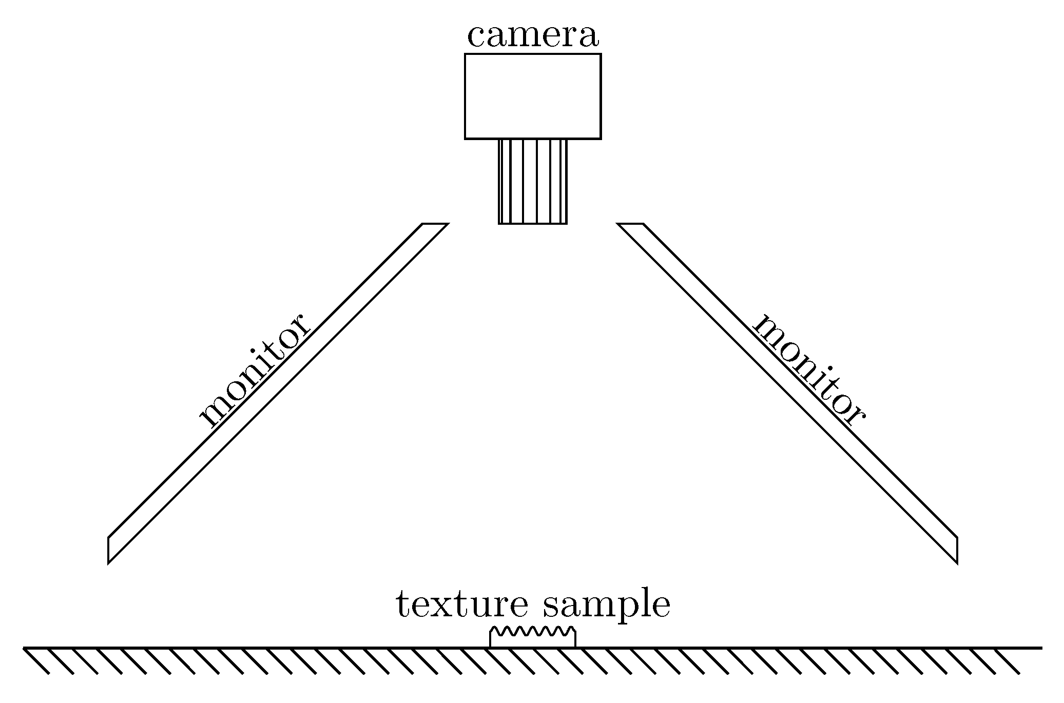
To generate the 46 illumination conditions, two computer monitors have been used as light sources (two 22-inch Samsung SyncMaster LED monitors). The monitors were tilted by 45 degrees facing down towards the texture sample, as shown in Figure 3. By illuminating different regions of one or both monitors it was possible to set the direction of the light illuminating the sample. By changing the RGB values of the pixels it was also possible to control the intensity and the color of the light sources. To do so, both monitors have been preliminarily calibrated using a X-Rite i1 spectral colorimeter by setting their white point to D65.
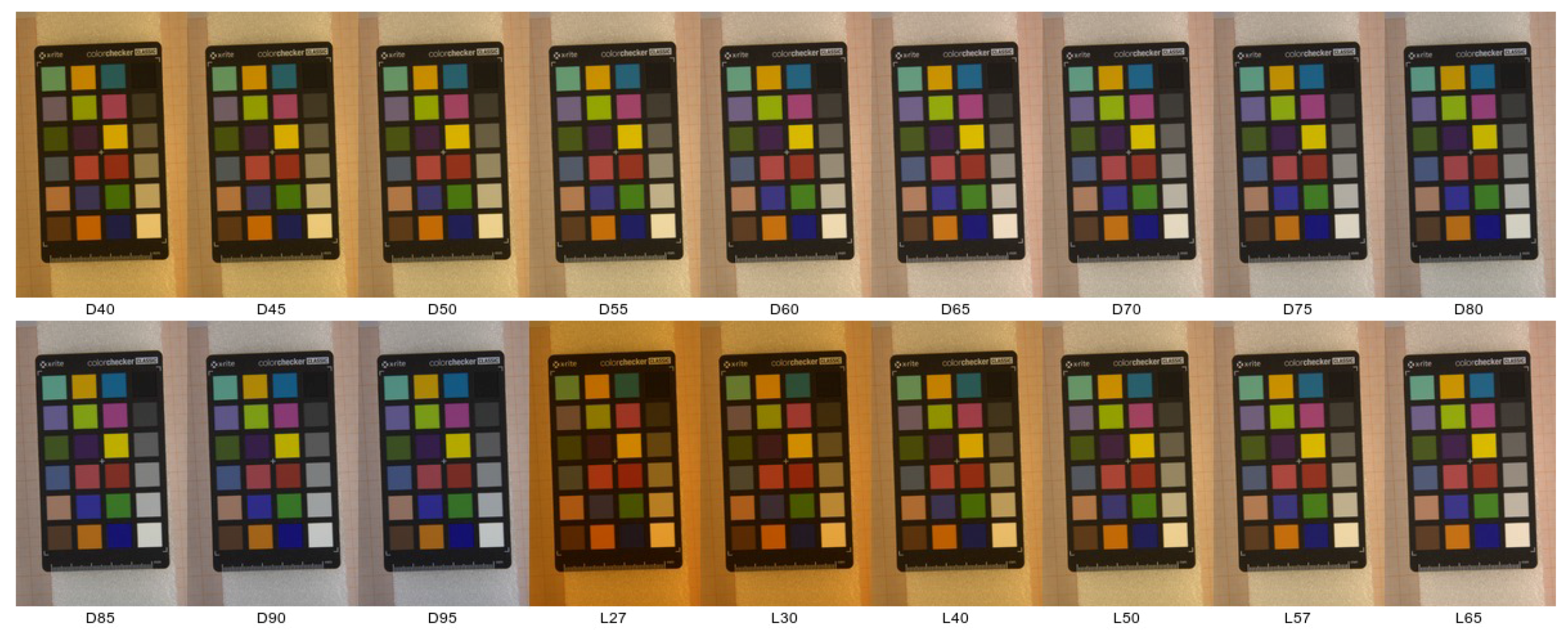
With this setup it was possible to approximate a set of diverse illuminants. In particular, 12 illuminants have been simulated, corresponding to 12 daylight conditions differing in the color temperature. The CIE- chromaticities corresponding to a given temperature T have been obtained by applying the following equations [44]:
where , , , if ≤ ≤ , and , , , if < . The chromaticities were then converted in the monitor RGB space [45] with a scaling of the color channels in such a way that largest value was 255.
The twelve daylight color temperatures that have been considered are: , , , …, (we will refer to these as D40, D45, ..., D95).
Similarly, six illuminants corresponding to typical indoor light have been simulated. To do so, the CIE- chromaticities of six LED lamps (six variants of SOLERIQ®S by Osram) have been obtained from the data sheets provided by the manufacturer. Then, again the RGB values were computed and scaled to 255 in at least one of the three channels. These six illuminants are referred to as L27, L30, L40, L50, L57, and L65 in accordance with the corresponding color temperature.
Figure 4 shows, for one of the classes, the 46 acquisitions corresponding to the 46 different lighting conditions in the RawFooT database. These include:
- 4 acquisitions with a D65 illuminant of varying intensity (100%, 75%, 50%, 25% of the maximum);
- 9 acquisitions which were only a portion of one of the monitors lit to obtain directional light (approximately 24, 30, 36, 42, 48, 54, 60, 66 and 90 degrees between the direction of the incoming light and the normal to the texture sample);
- 12 acquisitions with both monitors entirely projecting simulated daylight (D4, …, D95);
- 6 acquisitions with the monitor simulating artificial light (L27, ..., L65);
- 9 acquisitions with simultaneously change of both the direction and the color of light;
- 3 acquisitions with the two monitors simulating a different illuminant (L27+D65, L27+D95 and D65+D95);
- 3 acquisitions with both monitors projecting pure red, green and blue light.
In this work we are interested in particular in the effects of changes in the illuminant color. Therefore, we limited our analysis to the 12 illuminants simulating daylight conditions, and to the six simulating indoor illumination.
3.2. Color Balancing
An image acquired by a digital camera can be represented as a function mainly dependent on three physical factors: the illuminant spectral power distribution , the surface spectral reflectance , and the sensor spectral sensitivities . Using this notation, the sensor responses at the pixel with coordinates can be described as:
where is the wavelength range of the visible light spectrum, and and are three-component vectors. Since the three sensor spectral sensitivities are usually more sensitive respectively to the low, medium and high wavelengths, the three-component vector of sensor responses is also referred to as the sensor or camera raw RGB triplet. In the following we adopt the convention that triplets are represented by column vectors.
As previously said, the aim of color characterization is to derive the relationship between device-dependent and device-independent color representations for a given device. In this work, we employ an empirical, model-based characterization. The characterization model that transforms the i-th input device-dependent triplet into a device-independent triplet can be compactly written as follows [46]:
where is an exposure correction gain, M is the color correction matrix, I is the illuminant correction matrix, and denotes an element-wise operation.
Traditionally [46], M is fixed for any illuminant that may occur, while and I compensate for the illuminant power and color respectively, i.e.,
The model can be thus conceptually split into two parts: the former compensates for the variations of the amount and color of the incoming light, while the latter performs the mapping from the device-dependent to the device-independent representation. In the standard model (Equation (6)) is a single value, is a diagonal matrix that performs the Von Kries correction [47], and M is a matrix.
In this work, different characterization models have been investigated together with Equation (6) in order to assess how the different color characterization steps influence the texture recognition accuracy. The first tested model does not perform any kind of color characterization, i.e.,
The second model tested performs just the compensation for the illuminant color, i.e., it balances image colors as a color constancy algorithm would do:
The third model tested uses the complete color characterization model, but differently from the standard model given in Equation (6), it estimates a different color correction matrix for each illuminant j. The illuminant is compensated for both its color and its intensity, but differently from the standard model, the illuminant color compensation matrix for the j-th illuminant is estimated by using a different luminance gain for each patch i:
The fourth model tested is similar to the model described in Equation (9) but uses a larger color correction matrix by polynomially expanding the device-dependent colors:
where is an operator that takes as input the triplet and computes its polynomial expansion. Following [7], in this paper we use , i.e., the rooted second degree polynomial [38].
Summarizing, we have experimented with five color-balancing models. They all take as input the device-dependent raw values and process them in different ways:
- device-raw: it does not make any correction to the device-dependent raw values, leaving them unaltered from how they are recorded by the camera sensor;
- dcraw-srgb: it performs a full color characterization according to the standard color correction pipeline. The chosen characterization illuminant is the D65 standard illuminant, while the color mapping is linear and fixed for all illuminants that may occur. The correction is performed using the DCRaw software (available at http://www.cybercom.net/~dcoffin/dcraw/);
- linear-srgb: it performs a full color characterization according to the standard color correction pipeline, but using different illumination color compensation and different linear color mapping for each illuminant;
- rooted-srgb: it performs a full color characterization according to the standard color correction pipeline, but using a different illuminant color compensation and a different color mapping for each illuminant. The color mapping is no more linear but it is performed by polynomially expanding the device-dependent colors with a rooted second-degree polynomial.
The main properties of the color-balancing models tested are summarized in Table 1.
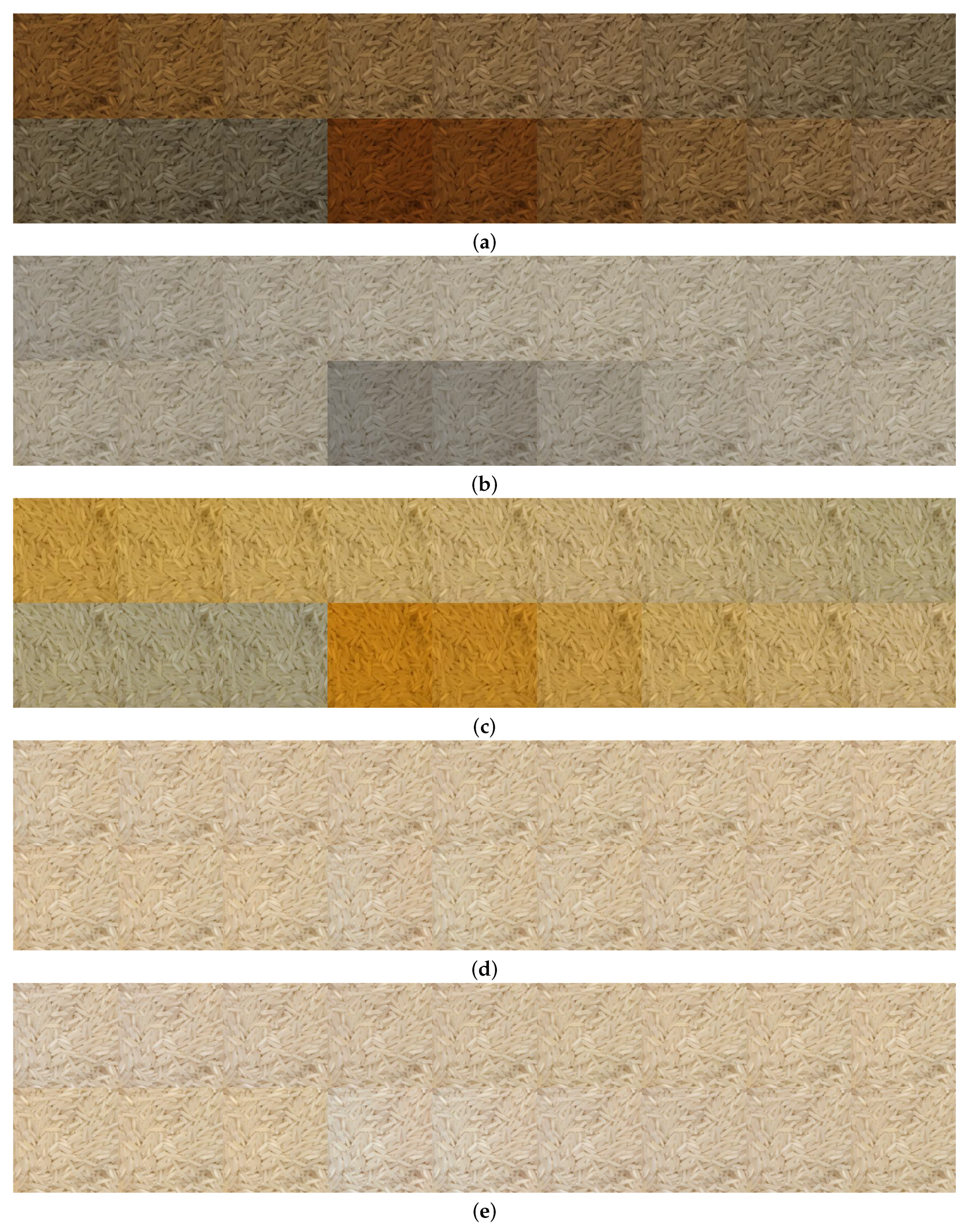
All the correction matrices for the compensation of the variations of the amount and color of the illuminant and the color mapping are found using the set of acquisitions of the Macbeth color checker available in the RawFooT using the optimization framework described in [7,36]. An example of the effect of the different color characterization models on a sample texture class of the RawFooT database is reported in Figure 6.
4. Experimental Setup
Given an image, the experimental pipeline includes the following operations: (1) color balancing; (2) feature extraction; and (3) classification. All the evaluations have been performed on the RawFooT database.
4.1. RawFooT Database Setup
For each of the 68 classes we considered 16 patches obtained by dividing the original texture image, that is of size 800 x 800 pixels, in 16 non-overlapping squares of size 200 × 200 pixels. For each class we selected eight patches for training and eight for testing alternating them in a chessboard pattern. We form subsets of patches by taking the training and test patches from images taken under different lighting conditions.
In this way we defined several subsets, grouped in three texture classification tasks.
- Daylight temperature: 132 subsets obtained by combining all the 12 daylight temperature variations. Each subset is composed of training and test patches with different light temperatures.
- LED temperature: 30 subsets obtained by combining all the six LED temperature variations. Each subset is composed of training and test patches with different light temperatures.
- Daylight vs. LED: 72 subsets obtained by combining 12 daylight temperatures with six LED temperatures.
4.2. Visual Descriptors
For the evaluation we select a number of descriptors from CNN-based approaches [51,52]. All feature vectors are -normalized (each feature vector is divided by its -norm.). These descriptors are obtained as the intermediate representations of deep convolutional neural networks originally trained for scene and object recognition. The networks are used to generate a visual descriptor by removing the final softmax nonlinearity and the last fully-connected layer. We select the most representative CNN architectures in the state of the art [53] by considering different accuracy/speed trade-offs. All the CNNs are trained on the ILSVRC-2012 dataset using the same protocol as in [1]. In particular we consider the following visual descriptors [10,54]:
- BVLC AlexNet (BVLC AlexNet): this is the AlexNet trained on ILSVRC 2012 [1].
- Medium CNN (Vgg M-2048-1024-128): it has three modifications of the Vgg M network, with a lower-dimensional last fully-connected layer. In particular we use a feature vector of 2048, 1024 and 128 size [51].
- Vgg Very Deep 19 and 16 layers (Vgg VeryDeep 16 and 19): the configuration of these networks has been achieved by increasing the depth to 16 and 19 layers, which results in a substantially deeper network than the previously ones [2].
- ResNet 50 is a residual network. Residual learning frameworks are designed to ease the training of networks that are substantially deeper than those used previously. This network has 50 layers [52].
4.3. Texture Classification
In all the experiments we used the nearest neighbor classification strategy: given a patch in the test set, its distance with respect to all the training patches is computed. The prediction of the classifier is the class of the closest element in the training set. For this purpose, after some preliminary tests with several descriptors in which we evaluated the most common distance measures, we decided to use the -distance: , where and are two feature vectors. All the experiments have been conducted under the maximum ignorance assumption, that is, no information about the lighting conditions of the test patches is available for the classification method and for the descriptors. Performance is reported as classification rate (i.e., the ratio between the number of correctly classified images and the number of test images). Note that more complex classification schemes (e.g., SVMs) would have been viable. We decided to adopt the simplest one in order to focus the evaluation on the features themselves and not on the classifier.
5. Results and Discussion
The effectiveness of each color-balancing model has been evaluated in terms of texture classification accuracy. Table 2 shows the average accuracy obtained on each classification task (daylight temperature, LED temperature and daylight vs LED) by each of the visual descriptors combined with each balancing model. Overall, the rooted-srgb and linear-srgb models achieve better performance than others models with a minimum improvement of about 1% and a maximum of about 9%. In particular the rooted-srgb model performs slightly better than linear-srgb. The improvements are more visible in Figure 7 that shows, for each visual descriptor, the comparison between all the balancing models. Each bar represents the mean accuracy over all the classification tasks. ResNet-50 is the best-performing CNN-based visual descriptor with a classification accuracy of 99.52%, that is about 10% better than the poorest CNN-based visual descriptor. This result confirms the power of deep residual nets compared to sequential network architectures such as AlexNet, and VGG etc.
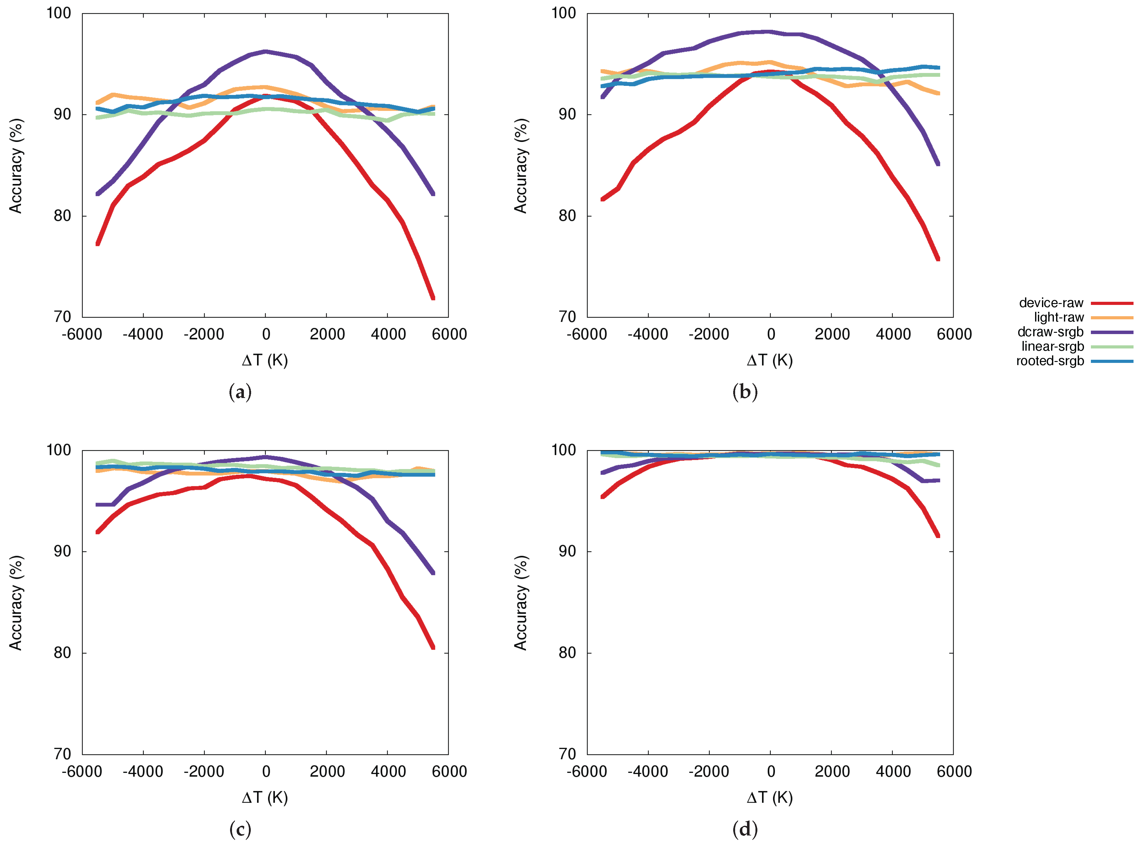
To better show the usefulness of color-balancing models we focused on the daylight temperature classification task, where we have images taken under 12 daylight temperature variations from 4000 K to 9500 K with an increment of 500 K. To this end, Figure 8 shows the accuracy behavior (y-axis) with respect to the difference ( measured in Kelvin degrees) of daylight temperature (x-axis) between the training and the test sets. The value corresponds to no variations. Each graph shows, given a visual descriptor, the comparison between the accuracy behaviors of each single model. There is an evident drop in performance for all the networks when is large and no color-balancing is applied. The use of color balancing is able to make uniform the performance of all the networks independently of the difference in color temperature. The dcraw-srgb model represents the most similar conditions to those of the ILSVRC training images. This explains why this model obtained the best performance for low values of . However, since dcraw-srgb does not include any kind of color normalization for high values of we observe a severe loss in terms of classification accuracy. Both linear-srgb and rooted-srgb are able, instead, to normalize the images with respect to the color of the illumination, making all the plots in Figure 8 almost flat. The effectiveness of these two models also depends on the fact that they work in a color space similar to those used to train the CNNs. Between the linear and the rooted models, the latter performs slightly better, probably because its additional complexity increases the accuracy in balancing the images.
6. Conclusions
Recent trends in computer vision seem to suggest that convolutional neural networks are so flexible and powerful that they can substitute in toto traditional image processing/recognition pipelines. However, when it is not possible to train the network from scratch due to the lack of a suitable training set, the achievable results are suboptimal. In this work we have extensively and systematically evaluated the role of color balancing that includes color characterization as a preprocessing step in color texture classification in presence of variable illumination conditions. Our findings suggest that to really exploit CNNs, an integration with a carefully designed preprocessing procedure is a must. The effectiveness of color balancing, in particular of the color characterization that maps device-dependent RGB values into a device-independent color space, has not been completely proven since the RawFooT dataset has been acquired using a single camera. As future work we would like to extend the RawFooT dataset and our experimentation acquiring the dataset using cameras with different color transmittance filters. This new dataset will make more evident the need for accurate color characterization of the cameras.
Acknowledgments
The authors gratefully acknowledge the support of NVIDIA Corporation with the donation of the Tesla K40 GPU used for this research.
Author Contributions
All the four authors equally contributed to the design of the experiments and the analysis of the data; all the four authors contributed to the writing, proof reading and final approval of the manuscript.
Conflicts of Interest
The authors declare no conflict of interest.
References
- Krizhevsky, A.; Sutskever, I.; Hinton, G.E. Imagenet classification with deep convolutional neural networks. In Advances in Neural Information Processing Systems; The MIT Press: Cambridge, MA, USA, 2012; pp. 1097–1105. [Google Scholar]
- Simonyan, K.; Zisserman, A. Very deep convolutional networks for large-scale image recognition. arXiv preprint arXiv:1409.1556 2014, 1–14. [Google Scholar]
- Zhou, B.; Lapedriza, A.; Xiao, J.; Torralba, A.; Oliva, A. Learning Deep Features for Scene Recognition using Places Database. In Advances in Neural Information Processing Systems 27; Neural Information Processing Systems (NIPS): Montreal, QC, Canada, 2014; pp. 487–495. [Google Scholar]
- Chen, Y.H.; Chao, T.H.; Bai, S.Y.; Lin, Y.L.; Chen, W.C.; Hsu, W.H. Filter-invariant image classification on social media photos. In Proceedings of the 23rd ACM International Conference on Multimedia, Brisbane, Australia, 26–30 October 2015. [Google Scholar]
- Gijsenij, A.; Gevers, T.; Van De Weijer, J. Computational color constancy: Survey and experiments. IEEE Trans. Image Process. 2011, 20, 2475–2489. [Google Scholar] [PubMed]
- Barnard, K.; Funt, B. Camera characterization for color research. Color Res. Appl. 2002, 27, 152–163. [Google Scholar] [CrossRef]
- Bianco, S.; Schettini, R. Error-tolerant Color Rendering for Digital Cameras. J. Math. Imaging Vis. 2014, 50, 235–245. [Google Scholar] [CrossRef]
- Bianco, S.; Schettini, R.; Vanneschi, L. Empirical modeling for colorimetric characterization of digital cameras. In Proceedings of the 2009 16th IEEE International Conference on Image Processing (ICIP), Cairo, Egypt, 7–10 November 2009. [Google Scholar]
- Cusano, C.; Napoletano, P.; Schettini, R. Evaluating color texture descriptors under large variations of controlled lighting conditions. J. Opt. Soc. Am. A 2016, 33, 17–30. [Google Scholar]
- Razavian, A.S.; Azizpour, H.; Sullivan, J.; Carlsson, S. CNN features off-the-shelf: An astounding baseline for recognition. In Proceedings of the 2014 IEEE Conference on Computer Vision and Pattern Recognition Workshops (CVPRW), Columbus, OH, USA, 23–28 June 2014. [Google Scholar]
- Russakovsky, O.; Deng, J.; Su, H.; Krause, J.; Satheesh, S.; Ma, S.; Huang, Z.; Karpathy, A.; Khosla, A.; Bernstein, M.; et al. ImageNet Large Scale Visual Recognition Challenge. Int. J. Comput. Vis. 2015, 115, 211–252. [Google Scholar] [CrossRef]
- Bianconi, F.; Harvey, R.; Southam, P.; Fernández, A. Theoretical and experimental comparison of different approaches for color texture classification. J. Electron. Imaging 2011, 20, 043006. [Google Scholar] [CrossRef]
- Palm, C. Color texture classification by integrative Co-occurrence matrices. Pattern Recognit. 2004, 37, 965–976. [Google Scholar] [CrossRef]
- Mäenpää, T.; Pietikäinen, M. Classification with color and texture: Jointly or separately? Pattern Recognit. 2004, 37, 1629–1640. [Google Scholar] [CrossRef]
- Seifi, M.; Song, X.; Muselet, D.; Tremeau, A. Color texture classification across illumination changes. In Proceedings of the Conference on Colour in Graphics, Imaging, and Vision, Joensuu, Finland, 14–17 June 2010. [Google Scholar]
- Cusano, C.; Napoletano, P.; Schettini, R. Combining local binary patterns and local color contrast for texture classification under varying illumination. J. Opt. Soc. Am. A 2014, 31, 1453–1461. [Google Scholar] [CrossRef] [PubMed]
- Cusano, C.; Napoletano, P.; Schettini, R. Local Angular Patterns for Color Texture Classification. In New Trends in Image Analysis and Processing – ICIAP 2015 Workshops; Murino, V., Puppo, E., Sona, D., Cristani, M., Sansone, C., Eds.; Springer International Publishing: Cham, Switzerland, 2015; pp. 111–118. [Google Scholar]
- Drimbarean, A.; Whelan, P. Experiments in colour texture analysis. Pattern Recognit. Lett. 2001, 22, 1161–1167. [Google Scholar] [CrossRef]
- Bianconi, F.; Fernández, A.; González, E.; Armesto, J. Robust color texture features based on ranklets and discrete Fourier transform. J. Electron. Imaging 2009, 18, 043012. [Google Scholar]
- LeCun, Y.; Bengio, Y.; Hinton, G. Deep learning. Nature 2015, 521, 436–444. [Google Scholar] [CrossRef] [PubMed]
- Cimpoi, M.; Maji, S.; Vedaldi, A. Deep filter banks for texture recognition and segmentation. In Proceedings of the IEEE Conference on Computer Vision and Pattern Recognition, Boston, MA, USA, 7–12 June 2015. [Google Scholar]
- Cusano, C.; Napoletano, P.; Schettini, R. Combining multiple features for color texture classification. J. Electron. Imaging 2016, 25, 061410. [Google Scholar] [CrossRef]
- Buchsbaum, G. A spatial processor model for object colour perception. J. Frankl. Inst. 1980, 310, 1–26. [Google Scholar] [CrossRef]
- Cardei, V.C.; Funt, B.; Barnard, K. White point estimation for uncalibrated images. In Proceedings of the Seventh Color Imaging Conference: Color Science, Systems, and Applications Putting It All Together, CIC 1999, Scottsdale, AZ, USA, 16–19 November 1999. [Google Scholar]
- Van de Weijer, J.; Gevers, T.; Gijsenij, A. Edge-based color constancy. IEEE Trans. Image Process. 2007, 16, 2207–2214. [Google Scholar] [CrossRef] [PubMed]
- Forsyth, D.A. A novel algorithm for color constancy. Int. J. Comput. Vis. 1990, 5, 5–35. [Google Scholar] [CrossRef]
- Gehler, P.V.; Rother, C.; Blake, A.; Minka, T.; Sharp, T. Bayesian color constancy revisited. In Proceedings of the 2008 IEEE Conference on Computer Vision and Pattern Recognition, Anchorage, AK, USA, 23–28 June 2008. [Google Scholar]
- Bianco, S.; Ciocca, G.; Cusano, C.; Schettini, R. Improving Color Constancy Using Indoor-Outdoor Image Classification. IEEE Trans. Image Process. 2008, 17, 2381–2392. [Google Scholar] [CrossRef] [PubMed]
- Bianco, S.; Cusano, C.; Schettini, R. Color Constancy Using CNNs. In Proceedings of the IEEE Conference on Computer Vision and Pattern Recognition Workshops (CVPRW), Boston, MA, USA, 7–12 June 2015. [Google Scholar]
- Bianco, S.; Cusano, C.; Schettini, R. Single and Multiple Illuminant Estimation Using Convolutional Neural Networks. IEEE Trans. Image Process. 2017. [Google Scholar] [CrossRef] [PubMed]
- McCamy, C.S.; Marcus, H.; Davidson, J. A color-rendition chart. J. App. Photog. Eng. 1976, 2, 95–99. [Google Scholar]
- ISO. ISO/17321-1:2006: Graphic Technology and Photography – Colour Characterisation of Digital Still Cameras (DSCs) – Part 1: Stimuli, Metrology and Test Procedures; ISO: Geneva, Switzerland, 2006. [Google Scholar]
- Finlayson, G.D.; Drew, M.S. Constrained least-squares regression in color spaces. J. Electron. Imaging 1997, 6, 484–493. [Google Scholar] [CrossRef]
- Vrhel, M.J.; Trussell, H.J. Optimal scanning filters using spectral reflectance information. In IS&T/SPIE’s Symposium on Electronic Imaging: Science and Technology; International Society for Optics and Photonics: San Jose, CA, USA, 1993; pp. 404–412. [Google Scholar]
- Bianco, S.; Bruna, A.R.; Naccari, F.; Schettini, R. Color correction pipeline optimization for digital cameras. J. Electron. Imaging 2013, 22, 023014. [Google Scholar] [CrossRef]
- Bianco, S.; Bruna, A.; Naccari, F.; Schettini, R. Color space transformations for digital photography exploiting information about the illuminant estimation process. J. Opt. Soc. Am. A 2012, 29, 374–384. [Google Scholar] [CrossRef] [PubMed]
- Bianco, S.; Gasparini, F.; Schettini, R.; Vanneschi, L. Polynomial modeling and optimization for colorimetric characterization of scanners. J. Electron. Imaging 2008, 17, 043002. [Google Scholar] [CrossRef]
- Finlayson, G.D.; Mackiewicz, M.; Hurlbert, A. Root-polynomial colour correction. In Proceedings of the 19th Color and Imaging Conference, CIC 2011, San Jose, CA, USA, 7–11 November 2011. [Google Scholar]
- Kang, H.R. Computational Color Technology; Spie Press: Bellingham, WA, USA, 2006. [Google Scholar]
- Schettini, R.; Barolo, B.; Boldrin, E. Colorimetric calibration of color scanners by back-propagation. Pattern Recognit. Lett. 1995, 16, 1051–1056. [Google Scholar] [CrossRef]
- Kang, H.R.; Anderson, P.G. Neural network applications to the color scanner and printer calibrations. J. Electron. Imaging 1992, 1, 125–135. [Google Scholar]
- Bianconi, F.; Fernández, A. An appendix to “Texture databases—A comprehensive survey”. Pattern Recognit. Lett. 2014, 45, 33–38. [Google Scholar] [CrossRef]
- Hossain, S.; Serikawa, S. Texture databases—A comprehensive survey. Pattern Recognit. Lett. 2013, 34, 2007–2022. [Google Scholar] [CrossRef]
- Wyszecki, G.; Stiles, W.S. Color Science; Wiley: New York, NY, USA, 1982. [Google Scholar]
- Anderson, M.; Motta, R.; Chandrasekar, S.; Stokes, M. Proposal for a standard default color space for the internet—sRGB. In Proceedings of the Color and imaging conference, Scottsdale, AZ, USA, 19–22 November 1996. [Google Scholar]
- Ramanath, R.; Snyder, W.E.; Yoo, Y.; Drew, M.S. Color image processing pipeline. IEEE Signal Process. Mag. 2005, 22, 34–43. [Google Scholar] [CrossRef]
- Von Kries, J. Chromatic adaptation. In Festschrift der Albrecht-Ludwigs-Universität; Universität Freiburg im Breisgau: Freiburg im Breisgau, Germany, 1902; pp. 145–158. [Google Scholar]
- Bianco, S.; Schettini, R. Computational color constancy. In Proceedings of the 2011 3rd European Workshop on Visual Information Processing (EUVIP), Paris, France, 4–6 July 2011. [Google Scholar]
- Nayatani, Y.; Takahama, K.; Sobagaki, H.; Hashimoto, K. Color-appearance model and chromatic-adaptation transform. Color Res. Appl. 1990, 15, 210–221. [Google Scholar] [CrossRef]
- Bianco, S.; Schettini, R. Two new von Kries based chromatic adaptation transforms found by numerical optimization. Color Res. Appl. 2010, 35, 184–192. [Google Scholar] [CrossRef]
- Chatfield, K.; Simonyan, K.; Vedaldi, A.; Zisserman, A. Return of the devil in the details: Delving deep into convolutional nets. arXiv preprint arXiv:1405.3531 2014, 1–11. [Google Scholar]
- He, K.; Zhang, X.; Ren, S.; Sun, J. Deep residual learning for image recognition. In Proceedings of the IEEE Conference on Computer Vision and Pattern Recognition, Seattle, WA, USA, 27–30 June 2016. [Google Scholar]
- Vedaldi, A.; Lenc, K. MatConvNet—Convolutional Neural Networks for MATLAB. CoRR 2014. [Google Scholar] [CrossRef]
- Napoletano, P. Hand-Crafted vs Learned Descriptors for Color Texture Classification. In International Workshop on Computational Color Imaging; Springer: Berlin, Germany, 2017; pp. 259–271. [Google Scholar]
- Zeiler, M.D.; Fergus, R. Visualizing and understanding convolutional networks. In Computer Vision–ECCV 2014; Springer: Berlin, Germany, 2014; pp. 818–833. [Google Scholar]
- Sermanet, P.; Eigen, D.; Zhang, X.; Mathieu, M.; Fergus, R.; LeCun, Y. Overfeat: Integrated recognition, localization and detection using convolutional networks. arXiv preprint arXiv:1312.6229 2013, 1–16. [Google Scholar]
Figure 1.
Example of correctly predicted image and mis-predicted image after a color cast is applied.
Figure 1.
Example of correctly predicted image and mis-predicted image after a color cast is applied.

Figure 2.
A sample for each of the 68 classes of textures composing the RawFooT database.
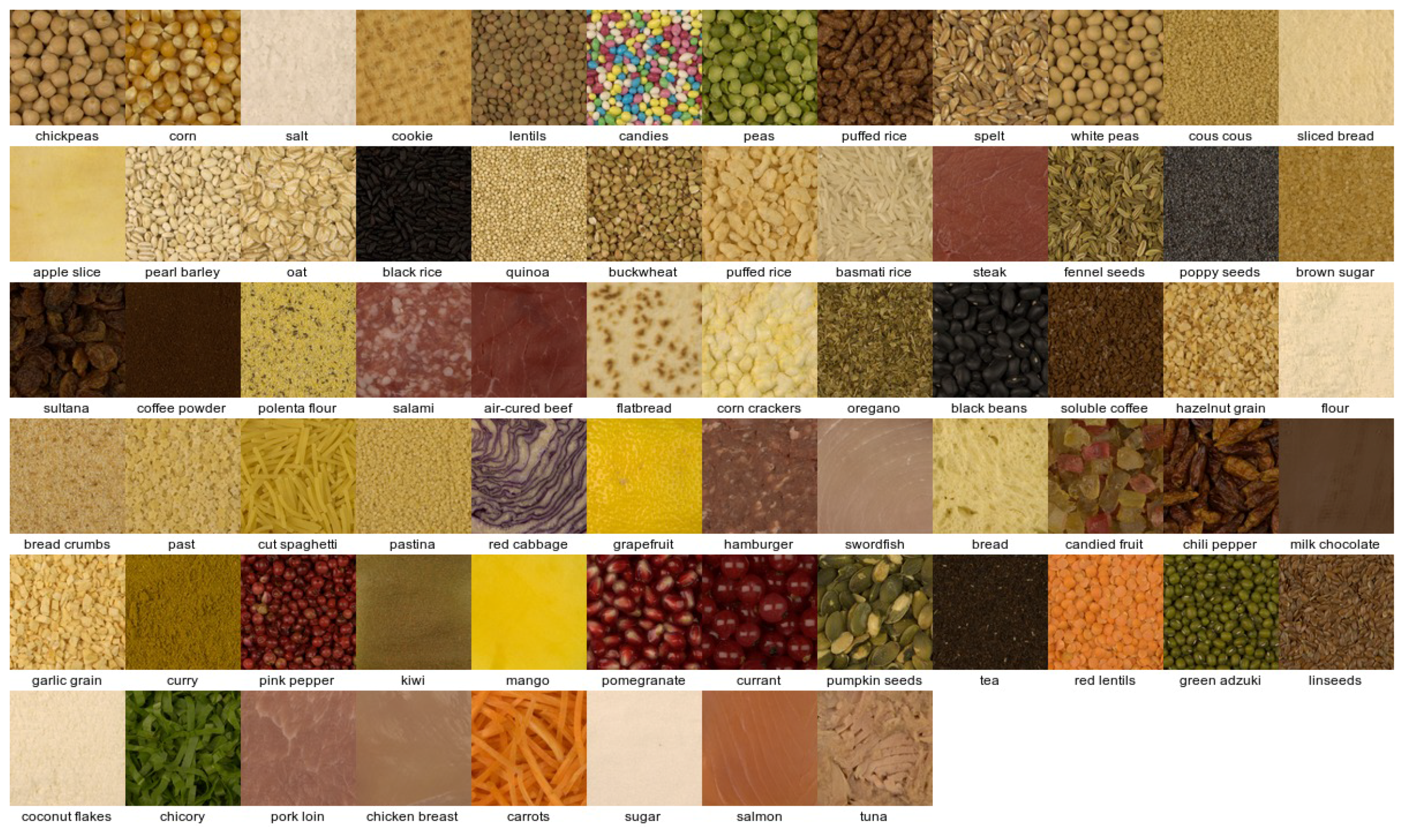
Figure 3.
Scheme of the acquisition setup used to take the images in the RawFooT database.

Figure 4.
Example of the 46 acquisitions included in the RawFooT database for each class (here the images show the acquisitions of the “rice” class).
Figure 4.
Example of the 46 acquisitions included in the RawFooT database for each class (here the images show the acquisitions of the “rice” class).
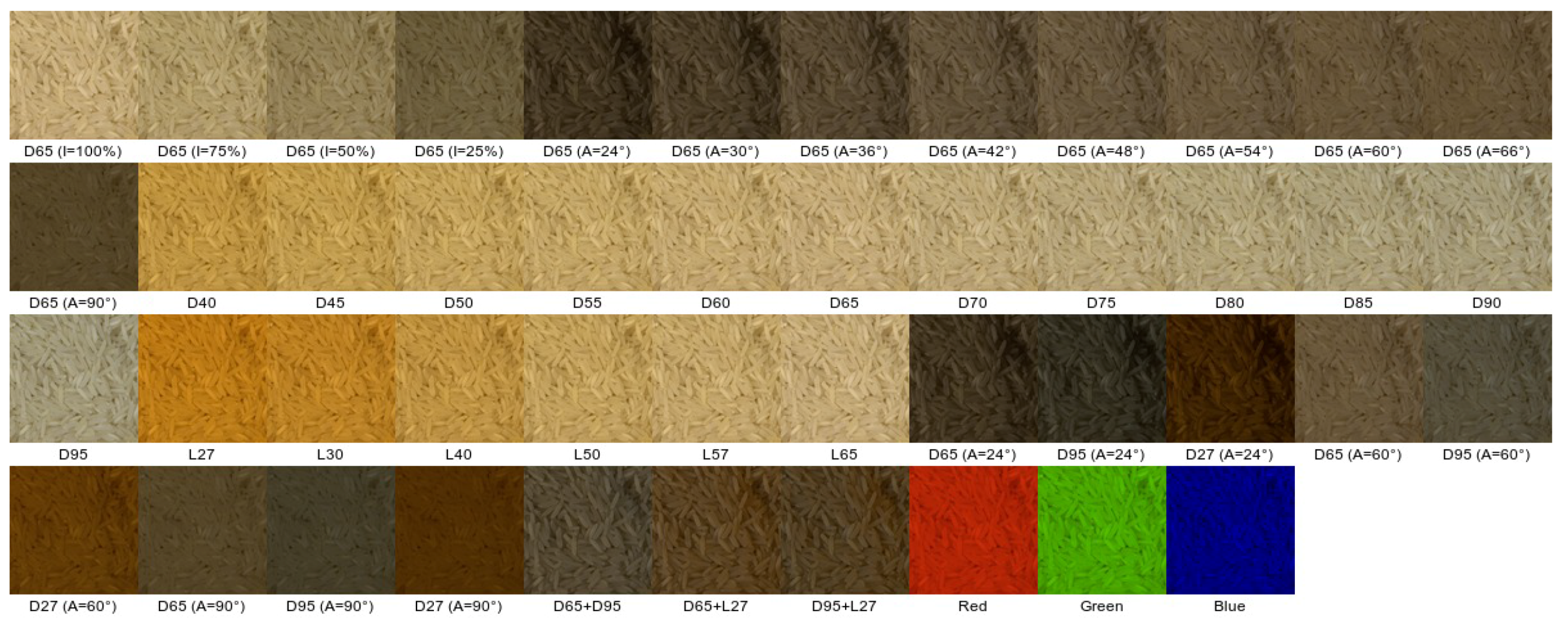
Figure 5.
The Macbeth color target, acquired under the 18 lighting conditions considered in this work.
Figure 5.
The Macbeth color target, acquired under the 18 lighting conditions considered in this work.

Figure 6.
Example of the effect of the different color-balancing models on the “rice” texture class: device-raw (a); light-raw (b); dcraw-srgb (c); linear-srgb (d); and rooted-srgb (e).
Figure 6.
Example of the effect of the different color-balancing models on the “rice” texture class: device-raw (a); light-raw (b); dcraw-srgb (c); linear-srgb (d); and rooted-srgb (e).

Figure 7.
Classification accuracy obtained by each visual descriptor combined with each model.
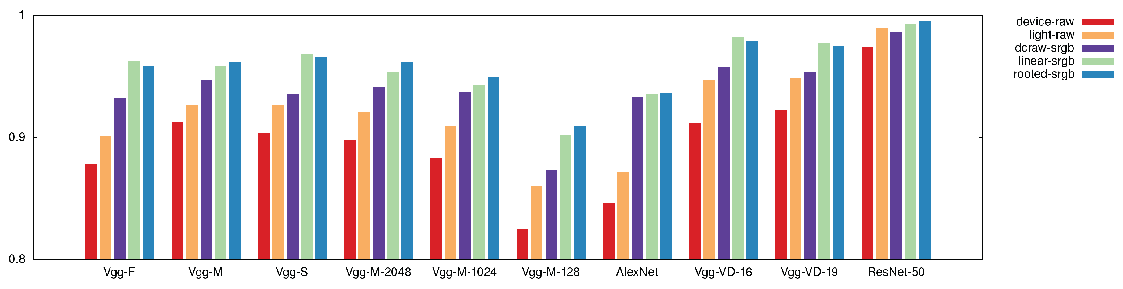
Figure 8.
Accuracy behavior with respect to the difference () of daylight temperature between the training and the test: (a) setsVGG-M-128; (b) AlexNet; (c) VGG-VD-16; (d) ResNet-50.
Figure 8.
Accuracy behavior with respect to the difference () of daylight temperature between the training and the test: (a) setsVGG-M-128; (b) AlexNet; (c) VGG-VD-16; (d) ResNet-50.


Table 1.
Main characteristics of the tested color-balancing models. Regarding the color-balancing steps, the open circle denotes that the current step is not implemented in the given model, while the filled circle denotes its presence. Regarding the mapping properties, the dash denotes that the given model does not have this property.
| Model Name | Color-Balancing Steps | Mapping Properties | |||
|---|---|---|---|---|---|
| Illum. Intensity | Illum. Color | Color | Mapping | Number | |
| Compensation | Compensation | Mapping | Type | of Mappings | |
| Device-raw (Equation (7)) | ○ | ○ | ○ | – | – |
| Light-raw (Equation (8)) | ○ | ● | ○ | – | – |
| Dcraw-srgb (Equation (6)) | ● | ◐ fixed for D65 | ● | Linear | 1 |
| Linear-srgb (Equation (9)) | ● | ● | ● | Linear | 1 for each illum. |
| Rooted-srgb (Equation (10)) | ● | ● | ● | Rooted 2nd-deg. poly. | 1 for each illum. |
Table 2.
Classification accuracy obtained by each visual descriptor combined with each model, the best result is reported in bold.
Table 2.
Classification accuracy obtained by each visual descriptor combined with each model, the best result is reported in bold.
| Features | Device-Raw | Light-Raw | Dcraw-Srgb | Linear-Srgb | Rooted-Srgb |
|---|---|---|---|---|---|
| VGG-F | 87.81 | 90.09 | 93.23 | 96.25 | 95.83 |
| VGG-M | 91.26 | 92.69 | 94.71 | 95.85 | 96.14 |
| VGG-S | 90.36 | 92.64 | 93.54 | 96.83 | 96.65 |
| VGG-M-2048 | 89.83 | 92.09 | 94.08 | 95.37 | 96.15 |
| VGG-M-1024 | 88.34 | 90.92 | 93.74 | 94.31 | 94.92 |
| VGG-M-128 | 82.52 | 85.99 | 87.35 | 90.17 | 90.97 |
| AlexNet | 84.65 | 87.16 | 93.34 | 93.58 | 93.68 |
| VGG-VD-16 | 91.15 | 94.68 | 95.79 | 98.23 | 97.93 |
| VGG-VD-19 | 92.22 | 94.87 | 95.38 | 97.71 | 97.51 |
| ResNet-50 | 97.42 | 98.92 | 98.67 | 99.28 | 99.52 |
© 2017 by the authors. Licensee MDPI, Basel, Switzerland. This article is an open access article distributed under the terms and conditions of the Creative Commons Attribution (CC BY) license (http://creativecommons.org/licenses/by/4.0/).
Share and Cite
MDPI and ACS Style
Bianco, S.; Cusano, C.; Napoletano, P.; Schettini, R. Improving CNN-Based Texture Classification by Color Balancing. J. Imaging 2017, 3, 33. https://doi.org/10.3390/jimaging3030033
AMA Style
Bianco S, Cusano C, Napoletano P, Schettini R. Improving CNN-Based Texture Classification by Color Balancing. Journal of Imaging. 2017; 3(3):33. https://doi.org/10.3390/jimaging3030033
Chicago/Turabian StyleBianco, Simone, Claudio Cusano, Paolo Napoletano, and Raimondo Schettini. 2017. "Improving CNN-Based Texture Classification by Color Balancing" Journal of Imaging 3, no. 3: 33. https://doi.org/10.3390/jimaging3030033
Note that from the first issue of 2016, this journal uses article numbers instead of page numbers. See further details here.