Enhancing Face Identification Using Local Binary Patterns and K-Nearest Neighbors


School of Communication Engineering, Hangzhou Dianzi University, Xiasha Higher Education Zone, Hangzhou 310018, China
*
Author to whom correspondence should be addressed.
J. Imaging 2017, 3(3), 37; https://doi.org/10.3390/jimaging3030037
Submission received: 21 March 2017
/
Revised: 28 August 2017
/
Accepted: 29 August 2017
/
Published: 5 September 2017
(This article belongs to the Special Issue Computer Vision and Pattern Recognition)
Abstract
:The human face plays an important role in our social interaction, conveying people’s identity. Using the human face as a key to security, biometric passwords technology has received significant attention in the past several years due to its potential for a wide variety of applications. Faces can have many variations in appearance (aging, facial expression, illumination, inaccurate alignment and pose) which continue to cause poor ability to recognize identity. The purpose of our research work is to provide an approach that contributes to resolve face identification issues with large variations of parameters such as pose, illumination, and expression. For provable outcomes, we combined two algorithms: (a) robustness local binary pattern (LBP), used for facial feature extractions; (b) k-nearest neighbor (K-NN) for image classifications. Our experiment has been conducted on the CMU PIE (Carnegie Mellon University Pose, Illumination, and Expression) face database and the LFW (Labeled Faces in the Wild) dataset. The proposed identification system shows higher performance, and also provides successful face similarity measures focus on feature extractions.
1. Introduction
Object recognition is a computer technology related to computer vision and image processing that deals with detecting and identifying humans, buildings, cars, etc., in digital images and video sequences. It is a huge domain including face recognition which basically has two different modes: verification and identification [1]. In this paper, we focus on the identification basic mode.
A face is a typical multidimensional structure and needs good computational analysis for recognition. The overall problem is to be able to accurately recognize a person’s identity and take some actions based on the outcome of the recognition process. Recognizing a person’s identity is important mainly for security reasons, but it could also be used to obtain quick access to medical, criminal, or any type of records. Solving this problem is important because it could allow people to take preventive action, provide better service in the case of a doctor appointment, allow users access to a secure area, and so forth.
Face identification is the process of identifying a person in a digital image or video, and showing their authentication identity. Identification is a one-to-many matching process that compares a query face image against all the template images inside the face database in order to determine the identity of the query face. Identification mode allows both positive and negative recognition outcomes, but the results are much more computationally costly if the template database is large [2,3]. Now, our goal is to determine which person inside the gallery—if any—is represented by the query face. More precisely, when a particular query image is submitted to the recognition system, the resulting normal map is compressed in order to compute its feature indexes, which are subsequently used to reduce the search to a cluster of similar normal maps selected through a visit in the k-d-tree [4].
In the past several years, academia and industry have developed many research works and practical approaches to overcome face recognition issues, specifically in pattern recognition and computer vision domains [5]. Facial recognition is a difficult problem due to the morphology of the face that can vary easily under the influence of many factors, such as pose, illumination, and expression [3]. In addition, faces have similar form and the same local parts (eyes, cheekbones, nose, lips, etc.). Therefore, to enhance the ability of a system to identify facial images, we need to apply an efficient algorithm that can describe the similarity representation and distinctive classification properties of diverse subject images.
As we mentioned above, local binary patterns (LBP) and k-nearest neighbor (K-NN) are among the famous proposed solutions available today.
For a decade, LBP was only used for texture classification; now it is also widely used to solve some of the common face recognition issues. LBP has many important properties, such as its robustness against any monotonic transformation of the gray scale, and its computational simplicity, which makes it possible to analyze images in challenging real-time settings [6].
The greater accuracy of k-nearest neighbor (K-NN) in image classification problems is highlighted; it is commonly used for its easier interpretation and low calculation time [7,8]. The main aim of LBP and K-NN in this work is to extract features and classify different LBP histograms, respectively, in order to ensure good matching between the extracted features histograms and provide a greater identification rate.
2. Prior Works
Over the past decades, there have been many studies and algorithms proposed to deal with face identification issues. Basically, the identification face is marked by similarity; authors in [9] measured the similarity between entire faces of multiple identities via Doppelganger List. It is claimed that the direct comparisons between faces are required only in similar imaging conditions, where they are actually feasible and informative. In the same way, Madeena et al. [10] presents a novel normalization method to obtain illumination invariance. The proposed model can recognize face images regardless of the face variations using a small number of features.
In [2], Sandra Mau et al. proposed a quick and widely applicable approach for converting biometric identification match scores to probabilistic confidence scores, resulting in increased discrimination accuracy. This approach works on 1-to-N matching of a face recognition system and builds on a confidence scoring approach for binomial distributions resulting from Hamming distances (commonly used in iris recognition).
In 2015, Pradip Panchal et al. [11] proposed Laplacian of Gaussian (LoG) and local binary pattern as face recognition solutions. In this approach, the extracted features of each face region are enhanced using LoG. In fact, the main purpose of LoG is to make the query image more enhanced and noise free. In our opinion, authors should use a Gaussian filter before applying LoG, since the combination of these two algorithms would provide better results than the ones obtained. Following the same way, authors in [12,13] also used LBP technique. In [12], the face recognition performance of LBP is investigated under different facial expressions, which are anger, disgust, fear, happiness, sadness, and surprise. Facial expression deformations are challenging for a robust face recognition system; thus, the study gives an idea about using LBP features to expression invariant. Further, authors in [13] implemented LBP and SSR (single scale retinex) algorithms for recognizing face images. In this work, lighting changes were normalized and the illumination factor from the actual image was removed by implementing the SSR algorithm. Then, the LBP feature extraction histograms could correctly match with the most similar face inside the database. The authors claimed that applying SSR and LBP algorithms gave powerful performance for illumination variations in their face recognition system.
Bilel Ameur et al. [14] proposed an approach where face recognition performance is significantly improved by combining Gabor wavelet and LBP for features extraction and, K-NN and SRC for classification. The best results are obtained in terms of time consumption and recognition rate; the proposed work also proved that the system efficiency depends on the size of the reduced vector obtained by the dimension reduction technique. However, Dhriti et al. [7] revealed the higher performance and accuracy of K-NN in classification images. In the same way as [7], authors in [8] used K-NN as the main classification technique and bagging as the wrapping classification method. Based on the powerful obtained outcomes, the proposed model demonstrated the performance and capabilities of K-NN to classify images.
Nowadays, research is not only focalized on face recognition in constrained environments; many authors also are trying to resolve face recognition in unconstrained environments.
The works [15,16,17] proposed a convolutional neural network (CNN) as a solution of the face recognition problem in unconstrained environments. Deep learning provides much more powerful capabilities to handle two types of variations; it is essential to learn such features by using two supervisory signals simultaneously (i.e., the face identification and verification signals), and the learned features are referred to as Deep IDentification-verification features (DeepID2) [15]. The paper showed that the effect of the face identification and verification supervisory signals on deep feature representation coincide with the two aspects of constructing ideal features for face recognition (i.e., increasing inter-personal variations and reducing intra-personal variations), and the combination of the two supervisory signals led to significantly better features than either one of them individually. Guosheng Hu et al. [16] presented a rigorous empirical evaluation of CNN based on face recognition systems. Authors quantitatively evaluated the impact of different CNN architectures and implementation choices on face recognition performances on common ground. The work [17] proposed a new supervision signal called center loss for face recognition task; the proposed center loss is used to improve the discriminative power of the deeply learned features. Combining the center loss with the softmax loss to jointly supervise the learning of CNNs, the discriminative power of the deeply learned features can be highly enhanced for robust face recognition.
3. Fundamental Background
3.1. CMU PIE & LFW Databases
Between October–December 2000, Terence Sim, Simon Baker, and Maan Bsat collected a database of over 40,000 facial images of 68 people. Using the Carnegie Mellon University 3D Room they imaged each person across 13 different poses, under 43 different illumination conditions, and with 4 different expressions (neutral, blinking/eyes closing, smiling, and talking). This database is called the CMU Pose, Illumination, and Expression (PIE) database [18]. The purpose of the PIE database is to evaluate facial recognition systems; it may also be used for facial feature detection, face pose estimation, and facial expression recognition.
LFW (Labeled Faces in the Wild) [19] is a database of face photographs designed for studying the problem of unconstrained face recognition. The LFW dataset contains 13,233 web-collected images from 5749 different identities, with large variations in poses, expressions, and illuminations.
3.2. Local Binary Patterns (LBP)
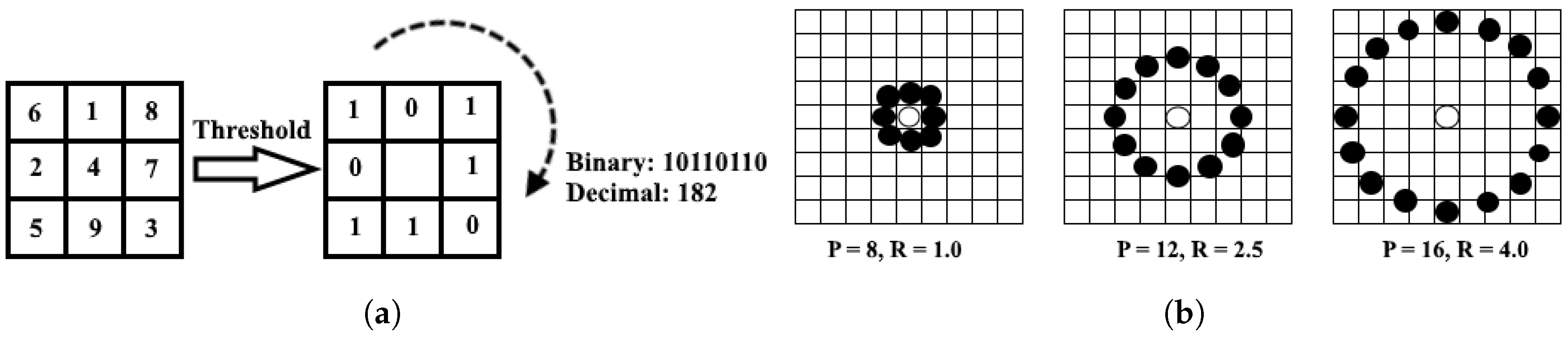
There are several methods for extracting unique and useful features from face images to perform face recognition; local binary pattern (LBP) is among the most popular ones, and it is also the most efficient and newest algorithm in that research field. First proposed by Ojala et al. in 1996 [20], the LBP operator is a signified robust method of texture description; it is described as an ordered set of binary comparisons of pixel intensities between the center pixel and its surrounding pixels. LBP was originally defined for neighborhoods, giving 8 bit codes based on the 8 pixels around the central one and representing the outcome as a binary number. LBP is derived for a specific pixel neighborhood radius R by comparing the intensities of P discrete circular sample points to the intensity of the center pixel (clockwise, counterclockwise), starting from a certain angle (as shown in Figure 1a). The comparison determines whether the corresponding location in the LBP of length M is “1” or “0”. The value “1” is assigned if the center pixel intensity is greater than or equal to the sample pixel intensity, and “0” otherwise (most commonly used with ); however, other values of the radius and sample numbers can be used (shown in Figure 1b). If a sample point is located between pixels, the intensity value used for comparison can be determined by bilinear interpolation.
3.2.1. Uniform Local Binary Patterns
Uniform LBP is an important case of LBP. An LBP descriptor is called uniform if it contains at most two circular bitwise 0–1 and 1–0 transitions. Since the allotted binary string needs to be considered as circular, the occurrence of only one transition is not possible; this means a uniform pattern has no transitions or two transitions. For instance, 00,000,000, 11,111,111, 11,011,111, and 10,001,111 are uniform binary patterns with zero bitwise transitions and two bitwise transitions, respectively. is a possible combination for uniform patterns with two bitwise transitions; it makes the work very easy compared to non-uniform patterns which have possible combinations. Instead of non-uniform binary patterns, there are two reasons for selecting uniform patterns. First, uniform LBP saves memory; for example, the number of possible patterns for a neighborhood of 8 pixels is 256 for standard LBP (non-uniform) and 59 for (u2 stands for using only uniform patterns), for 16 (interpolated) pixels is 65,536 for standard LBP and 243 for . The second reason is that it detects only the most important and useful features in the preprocessed images, such as corners, spots, edges, and line ends (Figure 2); thus, it can generate a more precise recognition rate and makes the process simpler and more effective.
3.2.2. Face Recognition Using Local Binary Patterns
Recently, LBP-based approaches have been proposed to solve certain face recognition problems, such as illumination and expression variations. It provides very good results in terms of both speed and discrimination performance.
The facial image texture is divided into several small blocks, from which the feature histogram (of each region) is constructed separately; therefore, the LBP histogram of each block will be combined to obtain a concatenated vector (a global histogram of the face). The similarity (distance) can then be measured by using the global histogram of different images. The global histogram of a facial image is represented by:
where is the global histogram and I is the LBP histogram of one block.
3.3. K-Nearest Neighbor Classification
As defined in Section 1, k-nearest neighbor has been used in statistical estimation and pattern recognition since the beginning of 1970s as a non-parametric technique; nowadays, it is commonly used for object classification. K-NN is a type of lazy learning algorithm where the function is only approximated locally and all computation is deferred until classification. The K-NN classifier has been best suited for classifying persons based on their images, due to its lesser execution time and better accuracy than other commonly used methods such as hidden Markov model and kernel method. Some methods like support vector machine (SVM) and Adaboost algorithms have proved to be more accurate than K-NN classifier, but the K-NN classifier has a faster execution time and it is more dominant than SVM [7].
Choosing the optimal value for K firstly depends upon inspecting the specific dataset; so, the K value is estimated using the available training sample observations. In general, a large K value is more precise as it reduces the overall noise in the classification, but there is no guarantee because it makes boundaries between classes less distinct. Cross-validation is one way to retrospectively determine a good K value by using an independent dataset to validate the K value; a good K can also be selected by various heuristic techniques. Historically, the optimal K for most datasets has been chosen as between 3 to 10; that produced much better results than 1-NN. In K-NN classification, the output is a class membership. An object is classified by a majority vote of its neighbors, with the object being assigned to the most common class among its k-nearest neighbors (K is a positive integer, typically small). The special case where the class is predicted to be the class of the closest training sample is called the nearest neighbor algorithm.
The training sets are vectors in a multidimensional feature space, each with a class label. The training phase of the algorithm consists only of storing the feature vectors and class labels of the training samples. In the classification phase, K is a user-defined constant, and an unlabeled vector (a query or test face image) is classified by assigning the label which is most frequent among the K training samples nearest to that specific query face. That means an image in the test set is recognized by assigning to it the label of the closest face inside the training set, so that the distance is measured between them. A commonly used distance metric is the Euclidean distance, which is often chosen for determining the closeness between the data points in K-NN; a distance is assigned between all pixels in a dataset. The distance defined as the Euclidean distance between two pixels is given by:
4. Proposed Approach
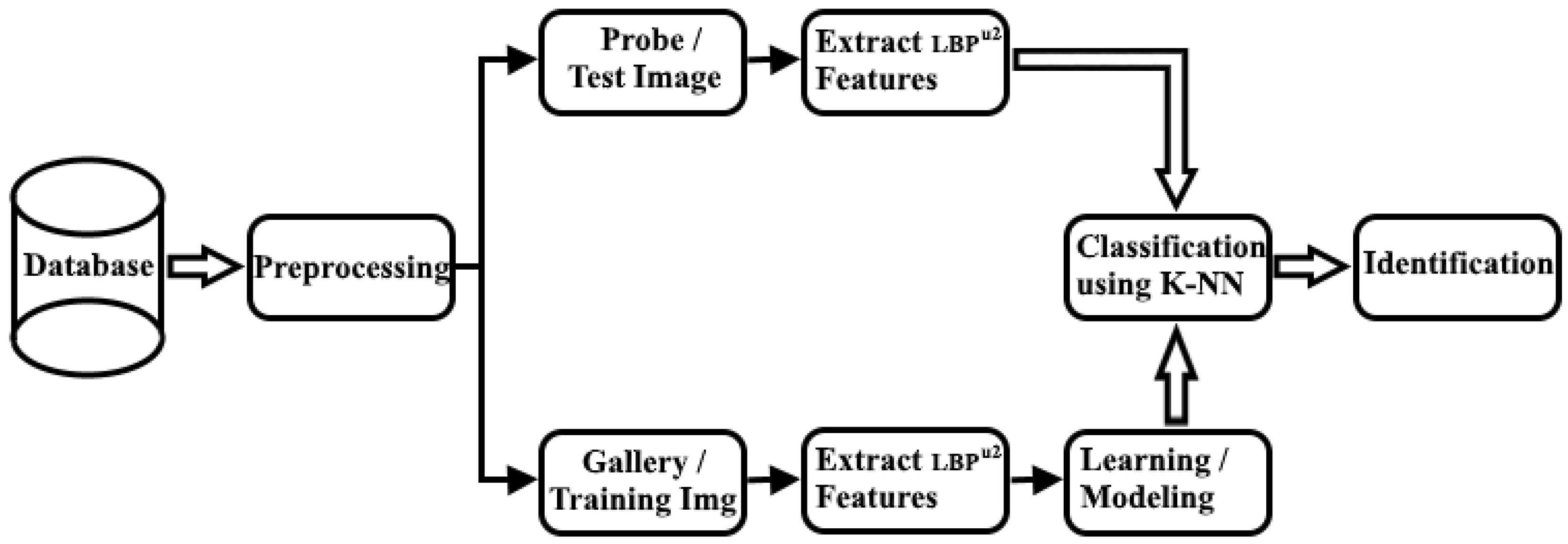
The proposed face identification system is based on the combination of the robust uniform local binary Ppattern and k-nearest neighbor. Face recognition is not a simple problem, since an unknown face image seen in the extraction phase is usually different from the face image seen in the classification phase. The main aim of this work is to solve the identification problem through face images which can vary easily under the influence of pose, illumination, and expression. The face image is divided into a grid of small non-overlapping regions, where the global LBP histogram of a particular face image is obtained by combining the histogram sequence of each non-overlapping region; explicitly, the global features are collected in single vector and therefore classified using the k-nearest neighbor algorithm. The Euclidean distance finds the minimum distance between histogram images. After comparing two individual histograms, if there is any similarity distance, it means they are related, and otherwise, not.
Figure 3 below displays our process diagram.
Our proposed system contains two principal stages before the junction:
- Start:
- Face database
- Preprocessing
- First stage:
- Input gallery images (training images)
- Collection of the extraction features using uniform LBP algorithm
- Learning or modeling via the LBP histogram
- Second stage:
- Input the probe or query image (test images)
- Collection of the extraction features using uniform LBP algorithm
- Junction:
- Classification using the K-NN algorithm with Euclidean distance
- End:
- Identification process
4.1. Preprocessing Phase
Consists of registering all images inside the database. The main aim of this phase is to improve the image data by suppressing unwanted distortions or enhancing important image features for further processing. Sometimes images have many lacks in contrast and brightness due to different limitations of imaging sub-systems and illumination conditions while capturing the image; techniques to resolve these issues include: contrast stretching, noise filtering, and histogram modification. Only noise filtering is applied in our work, after image registration. In definition, noise filtering is used to remove the unnecessary information from the image while preserving the underlying structure and the original texture under diverse lightning conditions. There are various types of filters available today, such as low-pass, high-pass, mean, median, etc.
Gaussian Filters Used as Low Pass Filters
One of the major problems that face recognition has to deal with is variations in illumination. Many studies have been explored to reduce, normalize, and ameliorate the effect caused by illumination variations. A Gaussian filter used as a low-pass filter is an appropriate method for carrying out illumination reduction and remove the lighting changes; its main purpose is to suppress all noise in the image. Another important property of Gaussian filters is that they are non-negative everywhere; this is important because most 1D signals vary about and can have either positive or negative values. Images are different in the sense that all values of one image are non-negative . Thus, convolution with a Gaussian filter guarantees a non-negative result, so the function maps non-negative values to other non-negative values ; the result is always another valid image. Digital images are composed of two frequency components: low (illumination) and high (noise). The Gaussian mathematical function implemented in this work is:
where is the Gaussian low-pass filter of size x and y, with standard deviation (positive).
4.2. Feature Extraction Phase
The LBP algorithm is a method of damage reduction technology that represents a discrimination of an interesting part of the face image in a compact feature vector. When the pre-processing phase is achieved, the LBP algorithm is applied to the segments in order to obtain a specific feature histogram. A focus on the feature extraction phase is essential because it has an observable impact on recognition system efficiency. The selection of our feature extraction method is the single most important factor to achieve higher recognition performance; that is why we used uniform LBP to extract useful features as it generates a more precise recognition rate and makes the process simpler and more effective. Hence, the application of suitable neighbor-sets for different values of needs to be done with utmost care.
4.3. Learning or Modeling Phase
Learning or modeling via LBP histogram is used to fit a model of the appearance of face images in the gallery, so that we can be able to know the discrimination between the faces of different subjects inside the database. In order to improve processing time, the extracted distance vectors are sorted in increasing order. In our framework, the learning step forms tightly packed conglomerates of visual feature histograms at detailed scales. These are determined by a form of configuration feature set, implying that the processing part reveals the similarity between features histograms. The characteristics of the processing part will be made explicit during matching in the classification phase.
4.4. K-NN Classifier
K-NN is the simplest of all machine learning and classification algorithms, and stores all available cases and classifies new cases based on a similarity measure. Therefore, the value K is used to perform classification by computing the simple histogram similarities. In this context, our good K value is selected by applying a K-fold cross-validation approach in order to estimate the optimum K. Further, each image of a set of visual features will find the best matching feature set between the test and all the training images.
5. Experiments and Results
To verify the robustness and optimum of our method, experiments were carried out on two huge databases: CMU PIE and LFW. Our proposed Algorithm 1 was conducted on an Intel Core i5-2430M CPU 2.40 GHz Windows 10 machine with 6 GB memory, and implemented in MATLAB R2016b. The performance of our proposed algorithm showed a powerful identification rate on the CMU PIE dataset.
| Algorithm 1: Proposed Algorithm |
|
Our face databases are very influential and common in studies of face recognition across pose, illumination, and expression variations. We used the image of the five nearly frontal poses (P05, P07, P09, P27, P29), a subset of 11,560 face images with 170 images per person on the CMU PIE dataset; and used around 6000 face images on the LFW dataset.
Firstly, we preprocessed our database due to the different illumination variations, and then applied the Gaussian filter before feature extractions in order to remove noises in the image to get a real LBP histogram of each image. Euclidian distance calculates the distance matrix between two images so that the image can be classified by a majority vote of its neighbors.
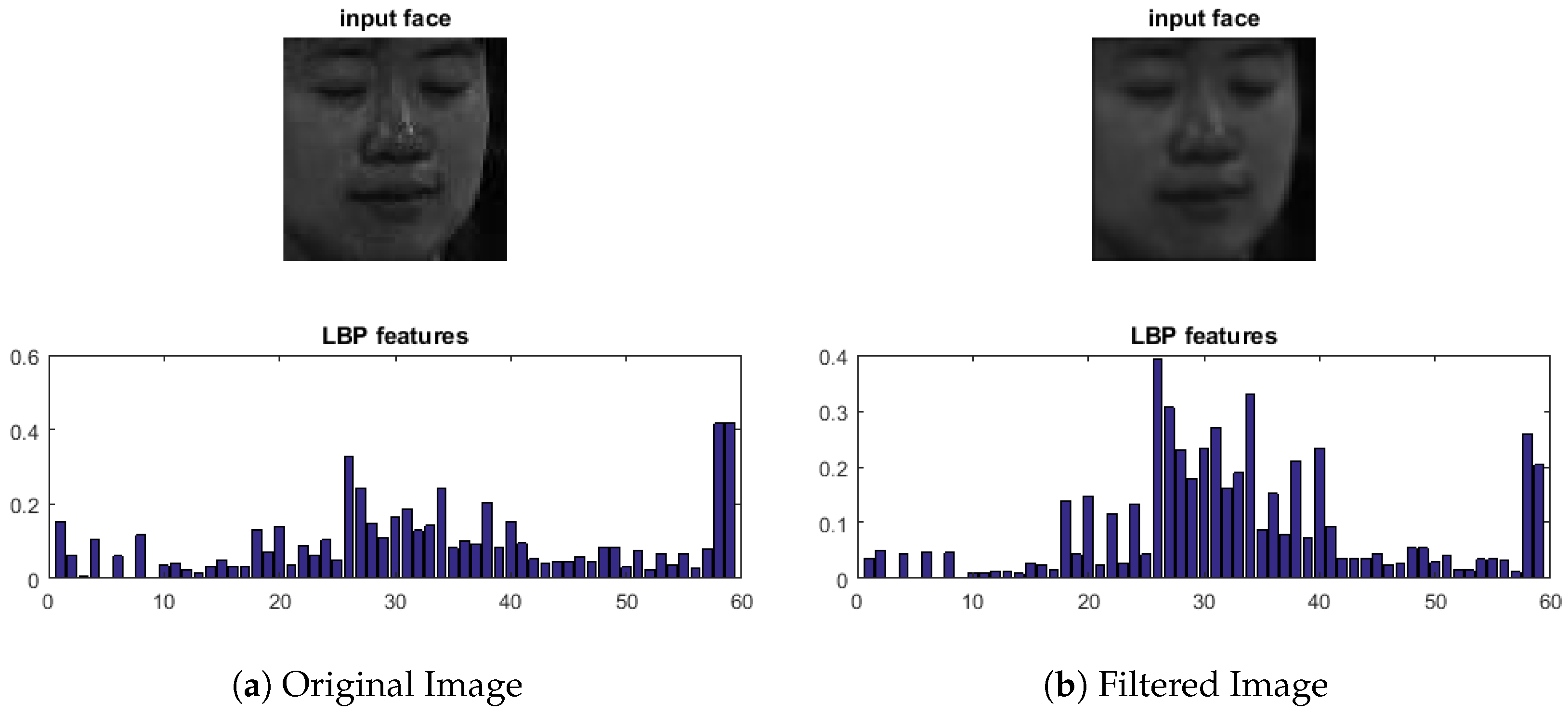
In our framework, we showed the performance of the Gaussian filter used as low-pass filter, which is an appropriate method for noise filtering. Here, the filter size used was different for each dataset. For the CMU PIE dataset we used as the size with , and as the size with for the LFW dataset. The higher filter size on LFW is due to the fact that it is an unconstrained or uncontrolled environment database and each image contains much more noise than images in a constrained or controlled environment (CMU PIE). Thus, the calculation and application of Gaussian parameters must be done with utmost care. After applying the filter, we obtain an enhanced image without noise; it is important to note that the Gaussian filter has the same role inside our databases. The filter size and are the same for all images inside a specific database. For instance, Figure 4 illustrates: Figure 4a is the image before applying the Gaussian filter (Original image), associated with its corresponding histogram; Figure 4b is the image after applying the Gaussian filter (Filtered image), with the corresponding histogram. The Gaussian filter removes all of the undesirable artifact (noise). Thus, we obtained an unmistakable image compared to Figure 4a. Moreover, the histograms in Figure 4a and Figure 4b are different; in Figure 4b, applying the filter is beneficial to get higher and more precise features (real histogram image without noise) than Figure 4a. Therefore, Gaussian’s difference can increase the visibility of edges and other details present in a digital image.
Figure 5 reveals the identification results of four people across the pose, illumination, and expression variations and accessories (wearing glasses). As we can see, all the subjects were correctly matched. Particularly, the subject in Figure 5a has a correct matching even in a reverse image, with incomplete face appearance and lighting change. Whereas, subjects in Figure 5b–d, displayed correct matching with different facial expressions: blinking and wearing glasses, talking, and smiling with lighting change, respectively.
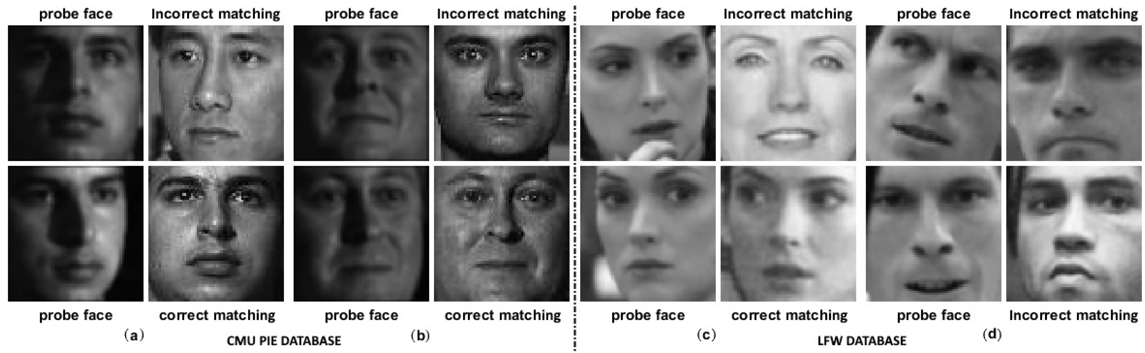
Finally, in Figure 6, the incorrect matching is less distinguishable—especially for the subject in Figure 6a,b, where the resemblance between probe image and gallery image (incorrectly matched) is extremely close. However, there are some cases where the failures are very blatant (Figure 6b,c), since the displayed images are chosen randomly inside the different sets.
For overall results, Table 1 describes the different outcomes obtained during the experiments. Maximum accuracy and powerful performance were achieved by implementing on CMU PIE (99.26%) and K = 4 on LFW (85.71%).
Table 2 and Table 3 describe the comparison of our results against many existing ones in both controlled and unconstrained environments, respectively.
The novelty in this research effort is that the combination of LBP, K-NN algorithms, and Gaussian filter is applied to increase and enhance our face identification rate. Furthermore, our method proved that the performance of the proposed model can be validated using one controlled environment database (CMU PIE). In order to reinforce our experiments, we used one unconstrained database (i.e., LFW). The obtained result shows that our proposed algorithm compared to the innovative solutions produced approximatively the same results.
6. Conclusions
The face plays a major role in our social intercourse in conveying identity, and the human ability to recognize faces is remarkable. The most difficult problem for today’s face recognition systems is to deal with face variation factors. In this study, the face image is first divided into several blocks, from which features are extracted using local binary patterns (LBP), then the global feature histogram of each face is constructed. Identification is performed using k-nearest neighbor (K-NN) classifier in the computer feature space Euclidean distance (D) as similarity measure. Before extracting features, we applied a Gaussian filter to the images in order to remove noise and normalize illumination variations; This made LBP extraction easier to correctly match the probe image with other images inside the database. The experiments showed that with achieved the maximum accuracy (99.26% on CMU PIE database). The simulation results indicate that the LBP features and K-NN classifier form a strong base for facial identification on unconstrained environment databases (85.71% on LFW dataset). Therefore, the unconstrained environment outcomes are opened for further analysis and may be improved upon.
Acknowledgments
This work was supported by the National Natural Science Foundation of China (No. 61372157)
Author Contributions
Idelette Laure Kambi Beli conceived, performed, and designed the experiments; analyzed the data; developed the analysis tools; and wrote the paper. Chunsheng Guo has fully supervised the work and approved the paper for submission.
Conflicts of Interest
The authors declare no conflict of interest.
References
- Ahonen, T.; Hadid, A.; Pietikainen, M. Face Recognition with Local Binary Patterns; Springer: Berlin/Heidelberg, Germany, 2004. [Google Scholar]
- Mau, S.; Dadgostar, F.; Lovell, B.C. Gaussian Probabilistic Confidence Score for Biometric Applications. In Proceedings of the 2012 International Conference Digital Image Computing Techniques and Applications (DICTA), Fremantle, WA, Australia, 3–5 December 2012. [Google Scholar]
- Jones, M.J. Face Recognition: Where We Are and Where to Go from Here. IEE J. Trans. Elect. Inf. Syst. 2009, 129, 770–777. [Google Scholar] [CrossRef]
- Abate, A.F.; Nappi, M.; Ricciardi, S.; Sabatino, G. One to Many 3D Face Recognition Enhanced Through k-d-Tree Based Spatial Access; Candan, K.S., Celentano, A., Eds.; Springer: Berlin/Heidelberg, Germany, 2005; pp. 5–16. [Google Scholar]
- Phillips, P.J.; Moon, H.; Rizvi, S.A.; Rauss, P.J. The FERET Evaluation Methodology for Face-Recognition Algorithms. IEEE Trans. Pattern Anal. Mach. Intell. 2000, 22, 1090–1104. [Google Scholar] [CrossRef]
- Rahim, A.; Hossain, N.; Wahid, T.; Azam, S. Face Recognition using Local Binary Patterns (LBP). Glob. J. Comput. Sci. Technol. 2013, 13, 469–481. [Google Scholar]
- Manvjeet Kaur, D. K-Nearest Neighbor Classification Approach for Face and Fingerprint at Feature Level Fusion. Int. J. Comput. Appl. 2012, 60, 13–17. [Google Scholar]
- Ebrahimpour, H.; Kouzani, A. Face Recognition Using Bagging KNN. In Proceedings of the International Conference on Signal Processing and Communication Systems (ICSPCS’2007), Gold Coast, Australia, 17–19 December 2007. [Google Scholar]
- Schroff, F.; Treibitz, T.; Kriegman, D.; Belongie, S. Pose, Illumination and Expression Invariant Pairwise Face-Similarity Measure via Doppelganger List Comparison. In Proceedings of the 2011 International Conference on Computer Vision, Barcelona, Spain, 6–13 November 2011. [Google Scholar]
- Sultana, M.; Gavrilova, M.; Yanushkevich, S. Expression, Pose, and Illumination Invariant Face Recognition using Lower Order Pseudo Zernike Moments. In Proceedings of the 2014 Intertional Conference of Computer Vision Theory and Applications (VISAPP), Lisbon, Portugal, 5–8 January 2014. [Google Scholar]
- Panchal, P.; Patel, P.; Thakkar, V.; Gupta, R. Pose, Illumination and Expression invariant Face Recognition using Laplacian of Gaussian and Local Binary Pattern. In Proceedings of the 5th Nirma University International Conference on Engineering (NUiCONE), Ahmedabad, India, 26–28 November 2015. [Google Scholar]
- Khorsheed, J.A.; Yurtkan, K. Analysis of Local Binary Patterns for Face Recognition Under Varying Facial Expressions. In Proceedings of the Signal Processing and Communication Application Conference 2016, Zonguldak, Turkey, 16–19 May 2016. [Google Scholar]
- Ali, A.; Hussain, S.; Haroon, F.; Hussain, S.; Khan, M.F. Face Recognition with Local Binary Patterns. Bahria Univ. J. Inf. Commu. Technol. 2012, 5, 46–50. [Google Scholar]
- Ameur, B.; Masmoudi, S.; Derbel, A.G.; Hamida, A.B. Fusing Gabor and LBP Feature Sets for KNN and SRC-based Face Recognition. In Proceedings of the 2nd International Conference on Advanced Technologies for Signal and Image Processing—ATSIP, Monastir, Tunisia, 21–23 March 2016. [Google Scholar]
- Sun, Y.; Wang, X.; Tang, X. Deep Learning Face Representation by Joint Identification-Verification. In Advances in Neural Information Processing Systems; MIT Press: Cambridge, MA, USA, 2014; pp. 1988–1996. [Google Scholar]
- Hu, G.; Yang, Y.; Yi, D.; Kittler, J.; Christmas, W.; Li, S.Z.; Hospedales, T. When Face Recognition Meets with Deep Learning: An Evaluation of Convolutional Neural Networks for Face Recognition. In Proceedings of the IEEE International Conference on Computer Vision Workshops 2015, Santiago, Chile, 7–13 December 2015. [Google Scholar]
- Wen, Y.; Zhang, K.; Li, Z.; Qiao, Y. A Discriminative Feature Learning Approach for Deep Face Recognition. In Proceedings of the European Conference on Computer Vision, Amsterdam, The Netherlands, 8–16 October 2016; Springer: Berlin/Heidelberg, Germany, 2016. [Google Scholar]
- Sim, T.; Baker, S.; Bsat, M. The CMU Pose, Illumination, and Expression (PIE) Database. In Proceedings of the Fifth IEEE International Conference on Automatic Face and Gesture Recognition (FGR’02), Washington, DC, USA, 21–21 May 2002. [Google Scholar]
- Labeled Faces in the Wild Homepage. Available online: http://vis-www.cs.umass.edu/lfw/ (accessed on 18 June 2017).
- Ojala, T.; Pietikäinen, M.; Harwood, D. A comparative study of texture measures with classification based on feature distributions. Pattern Recognit. 1996, 29, 51–59. [Google Scholar] [CrossRef]
Figure 1.
(a) The original local binary pattern (LBP) operator; (b) Circular neighbor-set for three different values of P, R.
Figure 1.
(a) The original local binary pattern (LBP) operator; (b) Circular neighbor-set for three different values of P, R.

Figure 2.
Different texture primitives detected by .
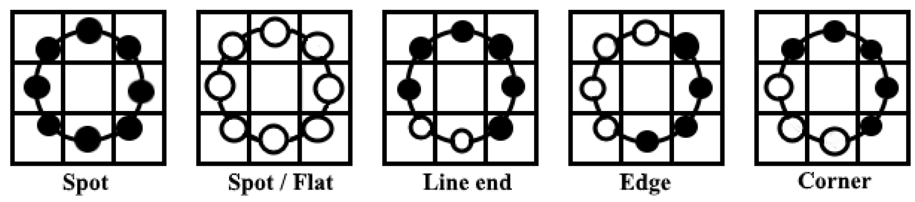
Figure 3.
Diagram of the process. K-NN: k-nearest neighbors.

Figure 4.
LBP histograms comparison.

Figure 5.
Correct identification. (a,b): CMU PIE; (c,d): LFW.
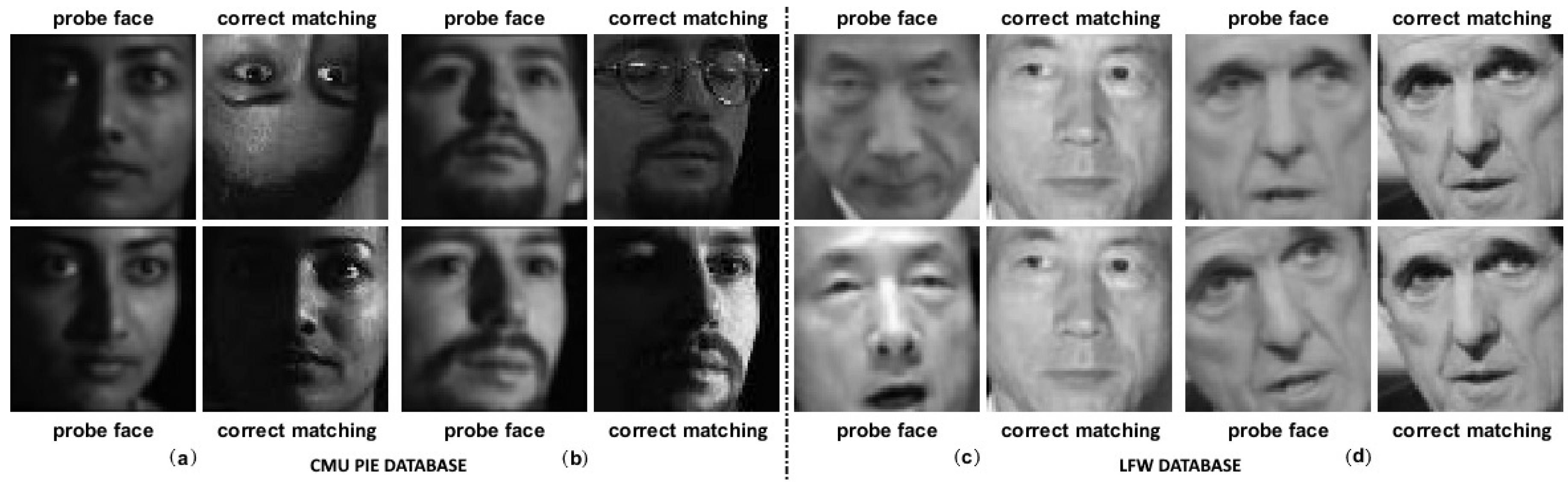
Figure 6.
Incorrect vs. correct matching.(a,b): CMU PIE; (c,d): LFW.

Table 1.
Identification rate.
| Databases | K | Identification Rate (%) | |
|---|---|---|---|
| CMU PIE | 22, 4 | 4 | 99.26 |
| LFW | 14, 4 | 4 | 85.71 |
© 2017 by the authors. Licensee MDPI, Basel, Switzerland. This article is an open access article distributed under the terms and conditions of the Creative Commons Attribution (CC BY) license (http://creativecommons.org/licenses/by/4.0/).
Share and Cite
MDPI and ACS Style
Kambi Beli, I.L.; Guo, C. Enhancing Face Identification Using Local Binary Patterns and K-Nearest Neighbors. J. Imaging 2017, 3, 37. https://doi.org/10.3390/jimaging3030037
AMA Style
Kambi Beli IL, Guo C. Enhancing Face Identification Using Local Binary Patterns and K-Nearest Neighbors. Journal of Imaging. 2017; 3(3):37. https://doi.org/10.3390/jimaging3030037
Chicago/Turabian StyleKambi Beli, Idelette Laure, and Chunsheng Guo. 2017. "Enhancing Face Identification Using Local Binary Patterns and K-Nearest Neighbors" Journal of Imaging 3, no. 3: 37. https://doi.org/10.3390/jimaging3030037
Note that from the first issue of 2016, this journal uses article numbers instead of page numbers. See further details here.