Novel Low Cost 3D Surface Model Reconstruction System for Plant Phenotyping


1
Arkansas Biosciences Institute, Arkansas State University, P.O. Box 639, State University, AR 72467, USA
2
Department of Computer Science, Arkansas State University, Jonesboro, AR 72401, USA
3
Department of Chemistry and Physics, Arkansas State University, P.O. Box 419, State University, AR 72467, USA
*
Author to whom correspondence should be addressed.
J. Imaging 2017, 3(3), 39; https://doi.org/10.3390/jimaging3030039
Submission received: 31 July 2017
/
Revised: 31 August 2017
/
Accepted: 7 September 2017
/
Published: 18 September 2017
(This article belongs to the Special Issue 2D, 3D and 4D Imaging for Plant Phenotyping)
Abstract
:Accurate high-resolution three-dimensional (3D) models are essential for a non-invasive analysis of phenotypic characteristics of plants. Previous limitations in 3D computer vision algorithms have led to a reliance on volumetric methods or expensive hardware to record plant structure. We present an image-based 3D plant reconstruction system that can be achieved by using a single camera and a rotation stand. Our method is based on the structure from motion method, with a SIFT image feature descriptor. In order to improve the quality of the 3D models, we segmented the plant objects based on the PlantCV platform. We also deducted the optimal number of images needed for reconstructing a high-quality model. Experiments showed that an accurate 3D model of the plant was successfully could be reconstructed by our approach. This 3D surface model reconstruction system provides a simple and accurate computational platform for non-destructive, plant phenotyping.
1. Introduction
One important question for plant phenotyping is how to measure the plants in three dimensions. Measurements such as leaf surface area, fruit volume, and leaf inclination angle are all vital to a non-destructive measurement of plant growth and stress tolerance. Three-dimensional (3D) model reconstruction allows this to be possible. In order to assess the morphological information of a fixed plant, 3D plant phenotyping is the method of choice. Moreover, 3D plant phenotyping also allows for researchers to gain a deeper understanding of plant architecture that can be used to improve traits such as light interception.
Current state of the art 3D reconstruction systems include hardware following the needs and the budget. In general, the hardware includes sensors and computation units. The sensors, which are the vital part of the system, are composed by various kinds of cameras and scanners, such as, LIDAR (Light Detection and Ranging), lasers, Time-of-Flight (ToF) cameras, and Microsoft RGB-D cameras. Image-based 3D modeling includes a stereo-vision system, space carving system, and a light field camera system, which all require more than one camera.
A comparison of current sensors for 3D reconstruction hardware systems is shown in Table 1. Each camera has its own advantage and limitations.
Laser line scanners (a.k.a. LIDAR) have proven their performance and show the greatest advantages for assessing plants. Kaminuma et al. [1] applied a laser range finder to reconstruct 3D models that represented the leaves and petioles as polygonal meshes, and then quantified the morphological traits from these models. Tumbo et al. [2] used ultrasonics in the field to measure citrus canopy volume. High throughput phenotyping of barley organs based on 3D laser scanning was presented in Paulus et al. [3]. This work showed the automatic parameter tracking of the leaves and stem of a barley plant on a temporal scale. Laser scanners are a useful tool for the acquisition of high-precision 3D point clouds of plants, but provide no information on volumetric and surface area, while having a poor resolution as well as long warm up time. A surface feature histogram based approach was adapted to image plants. Local geometric point features describe class characteristics, which were used to distinguish among different plant organs [4].
Stereo-vision was used to reconstruct the 3D surface of plants. A stereo-vision-based 3D reconstruction system for underwater scenes yielded promising depth map results in exploring underwater environments [5]. A combination of binocular stereo-vision [6] and structure-from-motion techniques [7] for the reconstruction of small plants from multiple viewpoints also showed good results. While the stereo-vision system is insensitive to movement and has color information, it also has poor depth resolution and is susceptible to sunlight. A low-cost and portable stereo-vision system was established to realize 3D imaging of plants under greenhouse cultivation [8]. A growth chamber system for 3D imaging by using a 3D-calibrated camera array was successfully used to quantify leaf morphological traits, 2D, and 3D leaf areas, and diurnal cycles of leaf movement; however, the limitation of this system is that it can only acquire half-shelf models, which lack detailed information about overlapping leaves [9]. A method for 3D reconstruction from multiple stereo cameras has been established, the boundary of each leaf patch was refined by using the level-set method, optimizing the model based on image information, curvature constraints, and the position of neighboring surfaces [10].
Space carving systems use multiple angles to reconstruct 3D model. For example, the reconstruction of thin structures based on silhouette constraints allows the preserving of fine structures, while the uniform voxel based data structure still limits the resolution [11]. For thin objects, volumetric approaches yield large amounts of empty space, implying the need for more efficient non-uniform data structures.
A light field camera system was used to phenotype large tomato plants in a greenhouse environment. Promising results of 3D reconstructed greenhouse scenes were shown in this work, along with several aspects related to camera calibration, lens aperture, flash illumination, and the limitation of the field of view [12].
Time-of-flight cameras and RGB-D sensors like the Kinect capture 3D information at a lower resolution. They have been also used in agriculture, however, are known to be less robust to bright illumination than stereo-vision systems. The time-of-flight (ToF) camera can measure depth information in real-time, and when this method [10] was used to align the depth scans in combination with a super-resolution approach, some mitigation of the sensor’s typically high signal noise level and systematic bias can be achieved [13].
ToF cameras have been typically used in combination with a red, green, and blue (RGB) camera. The ToF camera provided depth information, and the RGB camera was used to obtain color information. Shim et al. [14] presented a method to calibrate a multiple view acquisition system composed of ToF cameras and RGB color cameras. This system also has the ability to calibrate multi-modal sensors in real time.
There is a great deal of work that utilizes consumer-grade range camera technology (e.g., the Microsoft Kinect) [15] for scene reconstruction. The Kinect, which works in a similar way to a stereo camera, was originally designed for indoor video games. Due to its robustness and popularity, it is being studied for use in many research and industrial applications. In the study of Newcombe [16], the Kinect device was utilized to reconstruct dense indoor scenes. 3D plant analysis based on the mesh processing technique was presented in [17], where the authors created a 3D model of cotton from high-resolution images by using a commercial 3D digitization product named 3DSOM. Depth imaging systems use depth camera plus depth information to segment plants leaves and reconstruct plant models [18]. A depth camera was used to acquire images of sorghum and a semi-automated software pipeline was developed and used to generate segmented, 3D plant reconstructions from the images, and standard measures of shoot architecture such as shoot height, leaf angle, leaf length, and shoot compactness were measured from 3D plant reconstructions [19].
In summary, each system has its own advantages and limitations [20]. The use of current devices and systems is aimed at reducing the need for manual acquisition of phenotypic data while maintaining considerable cost [21]. Their functionality remains, to a greater or lesser extent, limited by the dynamic morphological complexity of plants [22]. There is not a 3D measurement system and method that solves all requirements, but one should choose based on the needs and available the budget.
In addition, plant architecture is usually complex, including large amounts of self-occlusion (leaves obscuring one another), and many smaller surfaces that appear similar. Therefore, how to measure plants in 3D in a non-destructive manner remains a serious challenge in plant phenotyping.
Aiming at providing a low cost solution to the above challenge, we present a fully automatic system to image-based 3D plant reconstruction. Our contributions include:
- A simple system: including a single RGB camera and a rotation stand.
- An automatic segmentation method: segmentation of plant objects was based on the open source PlantCV platform.
- A full view 3D model: a 3D reconstruction model was generated by using the structure-from motion method.
2. Materials and Methods
2.1. Hardware Setup
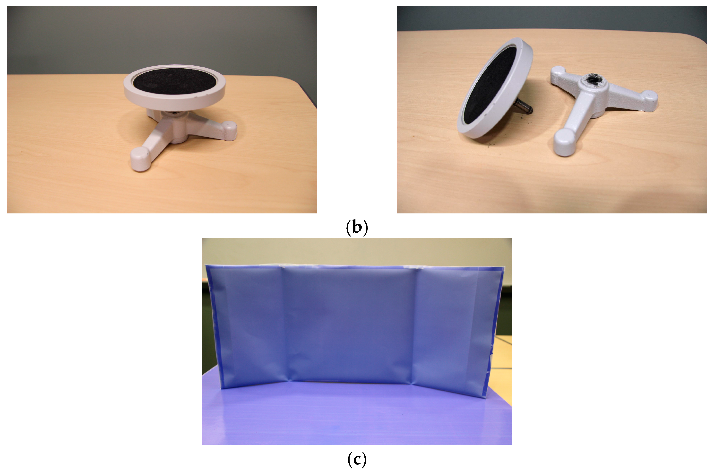
Our system was composed of a camera, a rotation stand, and a background plate. The model of the camera was Canon EOS REBEL SL1with ULTRASONIC EFS 17~85 mm f/4–5.6 IS USM lens, as shown in Figure 1a. The rotation stand was actually a small inoculating turntable, which can be accessed in most biological laboratories, as shown in Figure 1b. It was used to hold the plant and make it more stable when capturing multiple views from various angles. The background plate was a paper plate covered with blue poster, as shown in Figure 1c. We choose this background to ease extraction of the plant object in the subsequent segmentation step. We also used a camera tripod to hold and stabilize the camera when acquiring images.
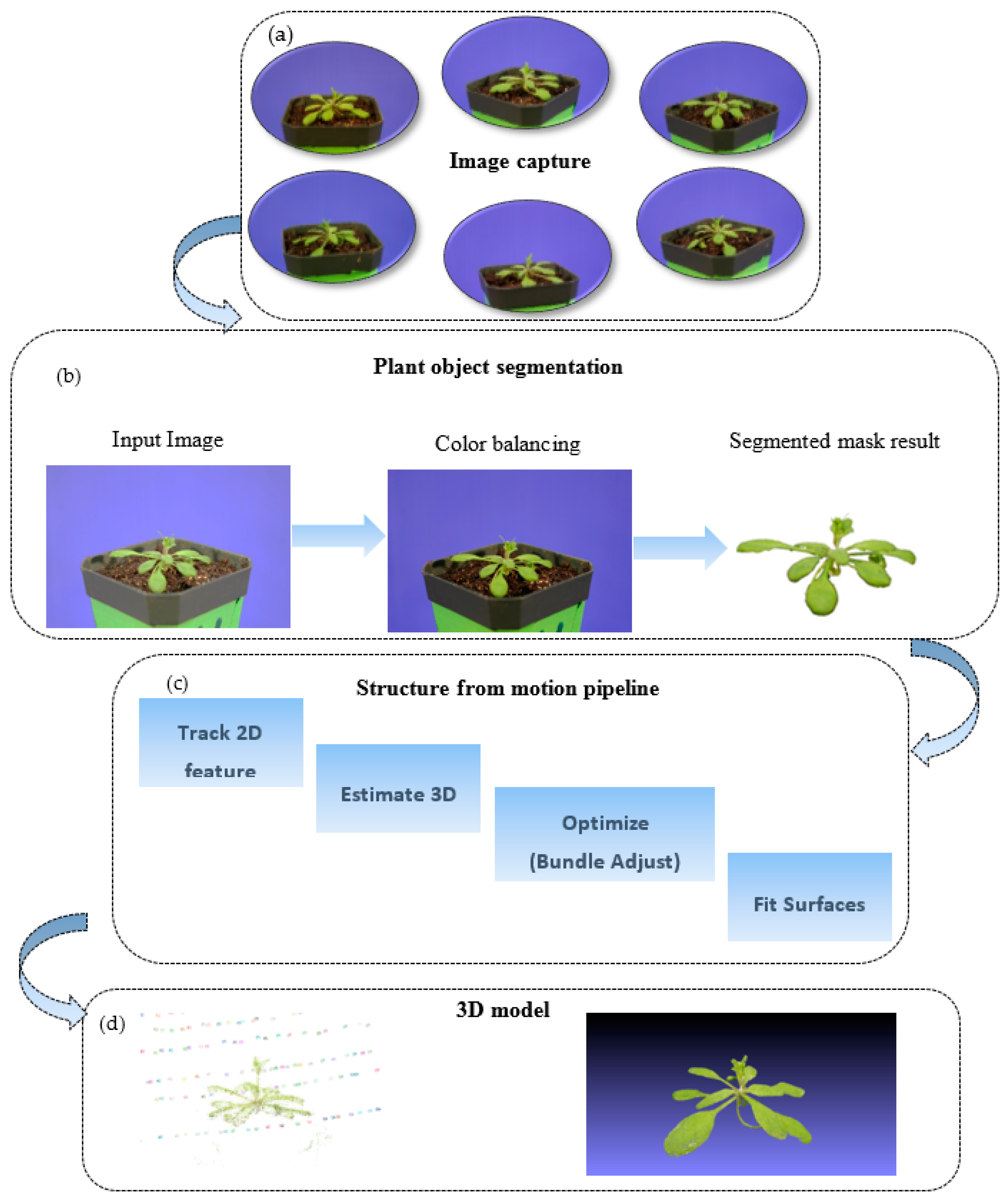
Our software method is illustrated in Figure 2. Based on our hardware platform, we captured a set of images from different viewpoints and angles in the image capture stage. Due to the illumination differences, we performed image quality enhancement using histogram equalization. Then, even-distributed color images with a better contrast were obtained during the image enhancement step. For each image, we segmented the plant from the background since our aim was to build a 3D model of the plant. Then we used the segmented plant images as input for our 3D surface modeling system, and applied the classic structure from the motion method to compute a 3D model. The reconstructed 3D model was represented in point cloud format. The detailed methods were illustrated as follows.
2.2. Image Acquisition
The setup of the experiments is shown in Figure 2, where the target plant is on the center of the rotation stand, and the camera is fixed at one position.
To make a full view reconstruction of the plant, multiple images from different view angles had to be taken over the target. The digital camera (shown in Figure 1) and a rotation stand were used to acquire images. In order to capture every angle of the target plant, we rotated the stand manually while keeping the camera fixed on the tripod.
A set of 1000 pictures with the resolution 3456 × 2304 of an Arabidopsis plant was acquired. The potted specimen was photographed indoors with stable illumination, avoiding movements caused by wind.
2.3. Plant Object Segmentation Based on PlantCV
Given the acquired images, we segmented the plants from the background. The rationale for this was to reduce the computational task for 3D model reconstruction. Generally, the acquired images include the plant objects as foreground and the rest as background. If the system is fed with images including both the foreground and the background, the system will compute all of the matching information inside of the scene, which will require a lot of time and computational resources, which could inevitably introduce computation error. Besides that, our goal in this paper was to reconstruct a plant model. Therefore, we used the segmented plant images as the input of our system.
We propose a plant object segmentation method based on the PlantCV (Plant Computer Vision) suite [23]. This is an open source platform to which multiple research teams, including ours, are contributing. An improved version of this platform, PlantCV 2.0 [24], is already available at http://plantcv.danforthcenter.org. The plant and the non-green background in acquired images were segmented by comparing the value of each pixel to a certain threshold in color space HSV (hue-saturation-value) and LAB (lightness-red/magenta and green- yellow and blue). This foreground segmentation technique is very fast and useful in our system, in which we need to segment the plant from the background.
We transformed the RGB channel images into different color space, such as HSV and LAB, and then we set up a threshold in each channel to segment the foreground plant object. R(x,y) in here represent the color value in specified channel, and (x,y) is the pixel value in image.
The detailed pseudo code is shown in Figure 3.
where are the input images and R(x,y) are the segmented result images. are the values from HSV and LAB color space.
2.4. Feature Points Detection and Matching
With the segmentation of the plant objects from different views, we needed to find the relationship between each of the two of them. First, we used a chessboard to estimate the camera intrinsic parameters, including the image dimension in pixels, the focal length, and the coordinates of the pixel intersected by the optical axis. Then, we needed to compute the feature points and its matching pairs among different view images.
We followed the Lowe’s method (SIFT). SIFT is quite an involved algorithm. We transformed an image into a large collection of feature vectors, each of which is invariant to image translation, scaling, and rotation, partially invariant to the illumination changes and robust to local geometric distortion.
Here’s an outline of what happens in SIFT.
- Constructing a scale space: This is the initial preparation. We create internal representations of the original image to ensure scale invariance.
- Laplacian of Gaussian (LoG) Approximation: The Laplacian of Gaussian is great for finding interesting points (or key points) in an image. LoG acts as a blob detector, which detects blobs in various sizes due to change in σ. In short, σ acts as a scaling parameter. For example, in some image, Gaussian kernel with low σ gives high value for small corner while Gaussian kernel with high σ fits well for larger corner. Since it is computationally expensive, we approximate it by using the representation created earlier.
- Finding keypoints: With the superfast approximation, we now try to find key points. These are the maxima and minima in the Difference of Gaussian image we calculate in Step 2. Once potential keypoints locations are found, they have to be refined to get more accurate results. They used Taylor series expansion of scale space to get a more accurate location of extreme, and if the intensity at this extreme is less than a threshold value, it is rejected.
- Get rid of bad key points: Edges and low contrast regions are bad keypoints. Eliminating these makes the algorithm efficient and robust. A technique similar to the Harris Corner Detector is used here. We know from the Harris corner detector that for edges, one Eigen value is larger than the other. So here, they used a simple function, if this ratio is greater than a threshold, that keypoints are discarded. So it eliminates any low-contrast keypoints and edge keypoints, and what remain are strong interest points.
- Assigning an orientation to the keypoints: An orientation is calculated for each key point. A neighborhood is taken around the keypoint location depending on the scale, the gradient magnitude, and the direction is calculated in that region. An orientation histogram with 36 bins, covering 360 degrees is created. Any further calculations are done relative to this orientation. This effectively cancels out the effect of orientation, making it rotation invariant. Also it contributes to stability of matching.
- Generate SIFT features: Finally, with scale and rotation invariance in place, one more representation is generated. This helps uniquely identify features. Now a keypoint descriptor is created. A 16 × 16 neighborhood around the keypoint is taken. It is divided into 16 sub-blocks of 4 × 4 size. For each sub-block, a 8 bin orientation histogram is created. So a total of 128 bin values are available. It is represented as a vector to from a keypoint descriptor.
- Keypoint Matching: Keypoints matching is done for a number of 2D images of a scene or object taken from different angles. This is used with bundle adjustment to build a sparse 3D model of the viewed scene and to simultaneously recover camera poses and calibration parameters. Then the position, orientation, and size of the virtual object are defined relative to the coordinate frame of the recovered model.
2.5. Dense 3D Reconstruction
In order to reconstruct the 3D model of the plants, we needed to compute the camera positions. Camera position was automatically recovered by the SFM (structure from motion) method. In this research, we use Bundler, which is a classical SFM system used to take a set of images, image features, and image matches as input, and then produce a 3D reconstruction of the camera and (sparse) scene geometry as output.
The process of the 3D reconstruction can be described as follows: First, the SIFT algorithm is employed to detect and describe image features in each image. The feature descriptors are used to find matches between the features in different images. Projective reconstruction and robust estimation techniques are employed to define the relative position between images, i.e., the position of the camera at each image acquisition. Once each camera pose is defined, a sparse 3D point cloud for the plant surface is produced based on feature matching.
We used the patch model developed by Furukawa and Ponce [25] to produce 3D dense reconstruction from multiple view stereo (MVS) data. Patches were reconstructed through feature matching, patch expansion, and patch filtering. The patches were used to build a polygonal mesh. Finally, a region growing a multiple view stereo technique is employed to produce a dense3D point cloud.
In addition, Poisson surface reconstruction is used to reform and smooth the point cloud in order to fix the quantization problem. The parameters used for this step are optimized and fixed at 16 for the number of neighbors in computing normals, 12 for octree depth, and 7 for solver divide in Poisson surface reconstruction.
2.6. Selecting the Optimal Image Numbers
When capturing plants images, the number of images captured is a key factor. It goes without saying that an increased number of images can provide more information about the plant, but meanwhile it will contain more redundant information due to the overlapping areas of the same surface. This affects the accuracy of the image feature matching procedure while performing the structure from motion step. If the matching errors accumulate with the number of images increase, it will greatly affect the quality of the reconstructed 3D models. On the contrary, if we decrease the number of images, the resultant 3D model lacks the necessary image information about the plant. For example, it is very difficult to reconstruct a 3D model of the plant from only 4 images that only cover limited viewpoints of the plant.
Based on the analysis above, theories about the relationship between multi-view data capturing and the quality of rendered virtual view were applied to find a balance between multi-view data capturing and the quality of the 3D model [26].
A camera model was established as shown in Figure 4. Each view is assumed to be captured by a pinhole camera under the ideal conditions. In Figure 4, an object is placed at a distance from the cameras. Each view with its capturing camera is evenly spaced on an arc in a circle with radius in the same pitch = . The resolution of capturing and rendering cameras is denoted as . It is limited by the highest spatial frequency of the scene.
Scene characters of the camera model include:
- Texture on the scene surface. Only the highest spatial frequency of the texture on the scene is considered since each camera of the multi-view capturing system can take images with spatial frequencies up to a certain limit, and this limit is dependent on such factors as the pixel pitch of the image sensor and focal length of the camera.
- Reflection property of the scene surface. An ideal Lambertian surface can ensure that the scene surface appears equally bright from all viewing directions and reflects all incident light while absorbing none.
- Depth range of the scene. All of the scene objects cover a depth range from minimum depth Zmin to maximum depth Zmax, and C is the converge center of cameras, as shown in Figure 1.
According to the deduction in [26], a proper number for reconstructing a three-dimensional surface model can be derived based on the following formulas:
where
We used this computation to calculate the optimal number of images needed to reconstruct a high quality 3D plant model.
3. Results and Discussion
Arabidopsis thaliana was chosen as our experiment plant since the characteristic overlapping leaves and flat architecture of the rosette present a challenge in reconstructing 3D models. This plant takes about 6 to 8 weeks to complete its entire life cycle and has a rapid growth rate [27]. Our capturing system consisted of a camera, a rotation stand and a background plate. The camera parameters are shown in Table 2.
The system reported by Pound et al. [10] is similar to the one proposed here, however, a main difference between that work on rice and wheat modeling, and our work is the model plant of choice. In our case Arabidopsis (Arabidopsis thaliana) is significantly smaller, with a flat canopy, and a presence of multiple overlapping leaves, presenting unique challenges to reconstruct a 3D model.
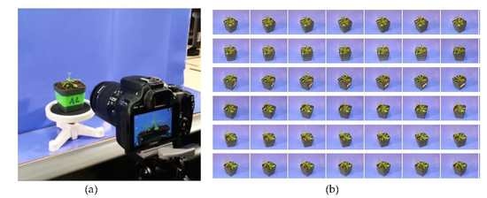
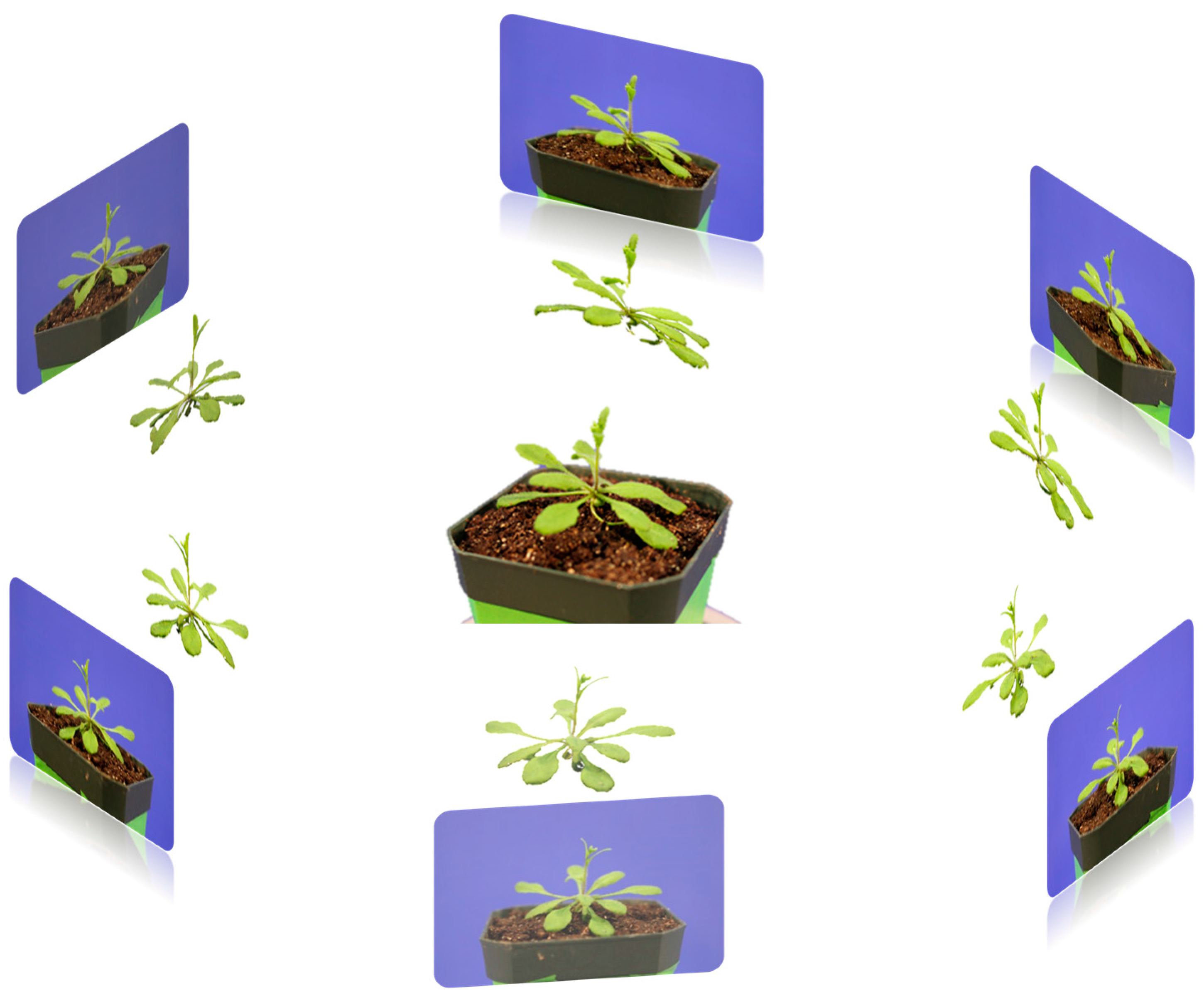
The plant was placed on a rotation stand which is shown in Figure 5a. Then, the camera was set at a fixed angle on the tripod to capture the images from different viewpoints. The stand was then rotated to capture every viewpoint of the plant at the same pitch angle. Then, the pitch angle of the camera was adjusted to capture another set of viewpoint images. The sample results of different viewpoint images are shown in Figure 5b. It is worth noticing that the capturing of images can also be achieved by a video camera with appropriate viewing angles. The video file needs to be converted as separated frames to be used as viewpoint images. In addition, users may choose to use a rotation stand equipped with a mechanical control device with accurate angle rotation, and in those cases, the acquired images could be analyzed with the method proposed here. We used a chessboard to perform the camera geometric calibration, and estimate the camera intrinsic parameters, including the image dimension in pixels, the focal length, and the coordinates of the pixel intersected by the optical axis. Other intrinsic parameters describing the radial and tangential lens distortion, including the radial distortion coefficient and tangential distortion coefficient were also computed by using Brown’s distortion model.
According to the deduction on how to select the optimal number of images, we calculated the optimal number of images needed for our experiment setup. The parameters needed are summarized in Table 3.
The depth range of our capturing scene was 0.15 m~0.45 m. As focal length of the lens is 50 mm, and the pixel pitch of the image sensor of the cameras is 320 µm, the resolution of each camera can be computed as 50 mm/320 µm = 156.25 cycles/rad. Capturing angles is equal to 2 × π, which is 360 degree. The calculation was detailed as follows:
where
During the development of this work, we captured multiple image sets of two-dozen Arabidopsis plants. In our experiments, the number of images ranged from 500 to 4000 per experiment. We chose 1000 as the optimal image number according to the deduction of theory and the visual quality of the resulting models. The capturing process used here is a simplified one. Image capturing can be easily automated by using an automatic rotating table. Another solution to avoid the labor-intensive image acquisition step is to capture a video while rotating the stand, and then the extraction of the required number of images for reconstruction. This is an approach we tested here, where 1000 images were extracted from the acquired video covering the different viewing angles of the plants.
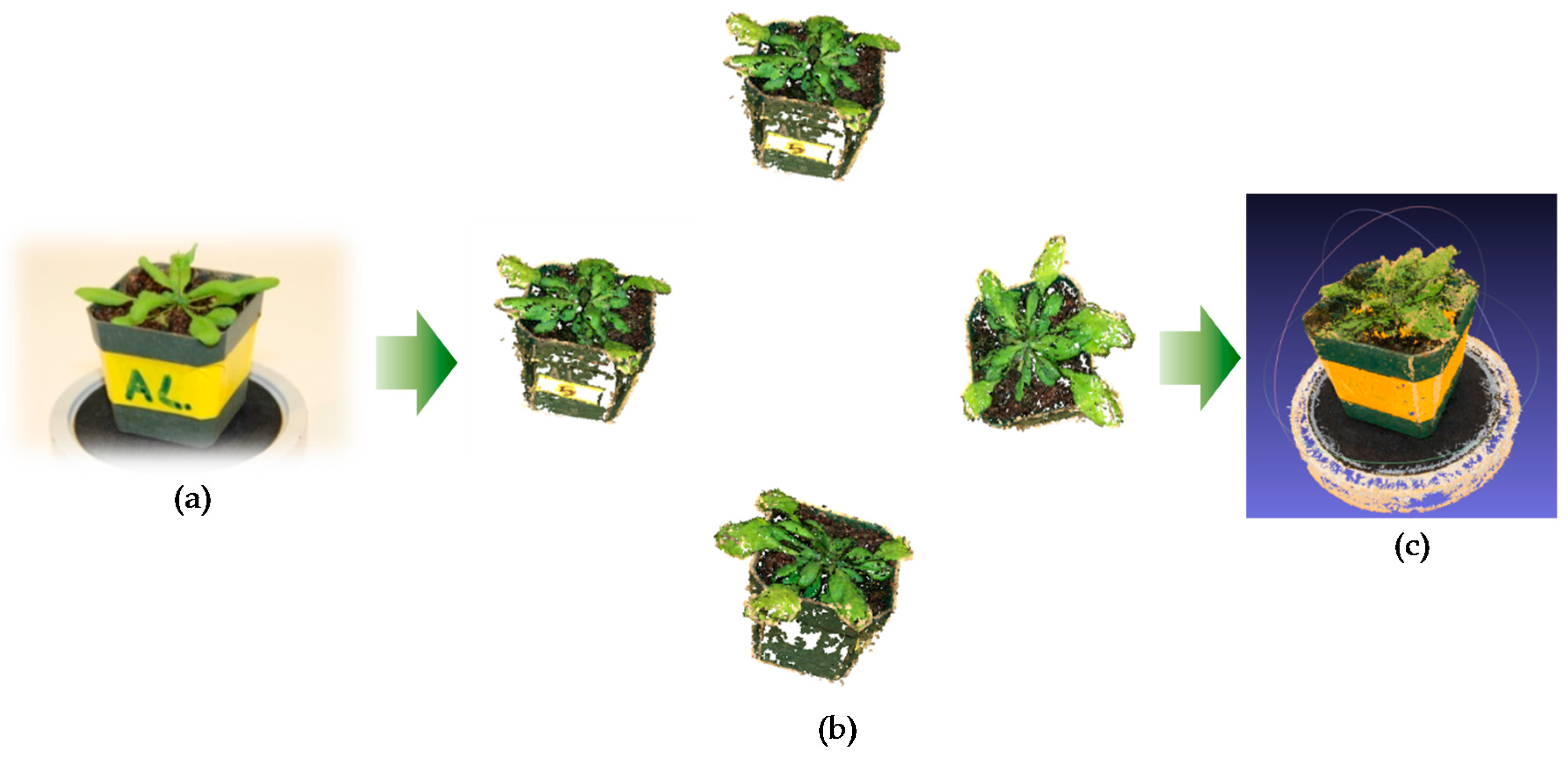
Given the acquired images, we were able to reconstruct 3D models of the plant by using the structure from motion method. In our initial experiments (Figure 6) where the number of captured images was relatively low, it could be clearly seen that the resulting 3D models were not satisfying as the plant objects had multiple defects, including holes on the leaves and a blurry boundary of the leaf surface.
To solve the above issues and improve the quality of the 3D models, the plant object was segmented from the background for all of the captured images. By segmenting the plant objects, the computation task for 3D model reconstruction was reduced, thus also greatly decreasing the mismatch error in the structure from motion step.
The plant object segmentation method was based on the PlantCV (Plant Computer Vision) suite. The plant and the non-green background in acquired images were then segmented by comparing the value of each pixel to a certain threshold in color space HSV (hue-saturation-value) and LAB (lightness-red/magenta and green- yellow and blue). We used 127, 90, and 83 for corresponding HSV channels. This segmentation method was applied to all of the captured images from different viewpoints, as shown in Figure 7. A sample of the plant object segmentation results is shown in Figure 8.
Using the data from the segmentation of plant objects from different views, Lowe’s method was applied to transform an image into a large collection of feature vectors and perform keypoints matching. Keypoints between two images were matched by identifying their nearest neighbors. In some cases, however, the second closest-match may be very near to the first. This may happen due to noise or other reasons. In this case, the ratio of closest-distance to second-closest distance was taken. If it was greater than 0.8, than they were rejected.
Then, based on the results from feature matching, a SFM (structure from motion) method was applied to reconstruct the 3D model of the plants. By using this method, we can compute the positions of the cameras, take image features and image matches as input, and produce a 3D reconstruction of the camera and scene geometry as output. The representation method of our 3D model was point cloud and it was stored in polygon format, which is used to store graphical objects that are described as a collection of polygons.
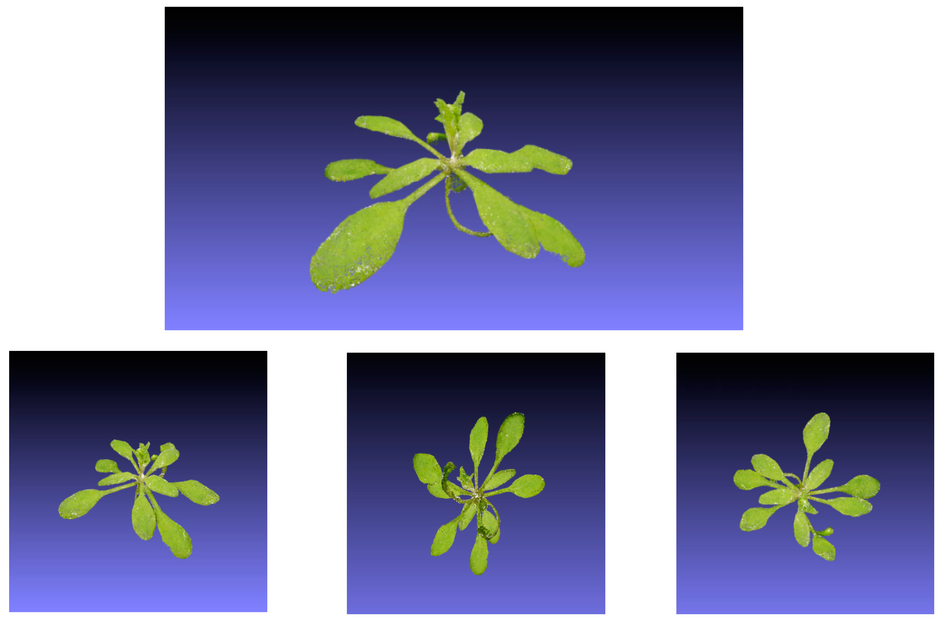
Illustrative images of the resulting 3D models are shown in Figure 9, which show the high quality of the reconstructed models. The details of the plants are reconstructed in a photorealistic manner, exhibiting smooth leaf areas and angles, which also include overlapping leaves, one of the most challenging features to model in Arabidopsis plants.
Visual inspection of the models we obtained (Figure 9), and those reported in the literature [28], indicate that our 3D models are of better quality as they are not missing details of the surface of leaves, petioles, or flower buds, despite the flat rosette architecture and the high number of overlapping leaves of the plant model are tested here. In some studies, validation of the 3D models has involved extracting 2D readouts and comparing those to the measurements obtained using manual destructive phenotyping. Another possible validation approach was the use of unique virtual datasets that has allowed authors to assess the accuracy of their reconstructions [10,11].
Future steps will involve automation of the system and implementation of the 3D models in the characterization of plants with enhanced growth rate, biomass accumulation, and improved tolerance to stress.
4. Conclusions
We present a system to generate image-based 3D plant reconstruction by using a single low-cost camera and a rotation stand. Our contribution includes: (1) a simple system: including an RGB camera and a rotation stand; (2) an automatic segmentation method where segmentation of the objects is based on the open source PlantCV platform; (3) a high quality 3D model: a full-view 3D reconstruction model was generated from the structure-from motion method; and, (4) the optimal number of images needed for the reconstruction of high quality models was deducted and computed. Experiments with Arabidopsis datasets successfully demonstrated the system’s ability to reconstruct 3D models of this plant with challenging architecture. This 3D surface model reconstruction system provides a low cost computational platform for non-destructive plant phenotyping. Our system can provide a good platform for plant phenotyping, including details such as leaf surface area, fruit volume, and leaf angles, which are vital to the non-destructive measuring of growth and stress on plant traits. Our software is built on an open source platform, which will be beneficial for the overall plant science community. The code is available at GitHub [29].
Acknowledgments
This work was supported by the Plant Imaging Consortium (PIC, http://plantimaging.cast.uark.edu/), funded by the National Science Foundation Award Numbers IIA-1430427 and IIA-1430428. We thank Zachary Campbell and Erin Langley for technical assistance and Jarrod Creameans for proofreading.
Author Contributions
Suxing Liu, Xiuzhen Huang, and Argelia Lorence conceived and designed the experiments; Suxing Liu performed the experiments; Suxing Liu and A. Lorence analyzed the data; Lucia M. Acosta-Gamboa grew plants and provided the idea of the rotating stand; Suxing Liu and Argelia Lorence wrote the manuscript.
Conflicts of Interest
The authors declare no conflict of interest.
References
- Kaminuma, E.; Heida, N.; Tsumoto, Y.; Yamamoto, N.; Goto, N.; Okamoto, N.; Konagaya, A.; Matsui, M.; Toyoda, T. Automatic quantification of morphological traits via three-dimensional measurement of Arabidopsis. Plant J. 2004, 38, 358–365. [Google Scholar] [CrossRef] [PubMed]
- Tumbo, S.D.; Salyani, M.; Whitney, J.D.; Wheaton, T.A.; Miller, W.M. Investigation of laser and ultrasonic ranging sensors for measurements of citrus canopy volume. ASABE 2002, 18, 367–372. [Google Scholar]
- Paulus, S.; Dupuis, J.; Riedel, S.; Kuhlmann, H. Automated analysis of barley organs using 3D laser scanning: An approach for high throughput phenotyping. Sensors 2014, 14, 12670–12686. [Google Scholar] [CrossRef] [PubMed]
- Paulus, S.; Dupuis, J.; Mahlein, A.K.; Kuhlmann, H. Surface feature based classification of plant organs from 3D laser scanned point clouds for plant phenotyping. BMC Bioinform. 2013, 14, 238. [Google Scholar] [CrossRef] [PubMed]
- Brandou, V.; Allais, A.; Perrier, M.; Malis, E.; Rives, P.; Sarrazin, J.; Sarradin, P.M. 3D reconstruction of natural underwater scenes using the stereovision system IRIS. In Proceedings of the Europe OCEANS, Aberdeen, UK, 18–21 June 2007; pp. 1–6. [Google Scholar]
- Ni, Z.; Burks, T.F.; Lee, W.S. 3D reconstruction of small plant from multiple views. In Proceedings of the ASABE and CSBE/SCGAB Annual International Meeting, Montreal, QC, Canada, 13–16 July 2014. [Google Scholar]
- Wu, C. Towards linear-time incremental structure from motion. In Proceedings of the 2013 International Conference on 3D Vision, Seattle, WA, USA, 29 June–1 July 2013; pp. 127–134. [Google Scholar]
- Li, D.; Xu, L.; Tang, X.S.; Sun, S.; Cai, X.; Zhang, P. 3D Imaging of greenhouse plants with an inexpensive binocular stereo vision system. Remote Sens. 2017, 9, 508. [Google Scholar] [CrossRef]
- An, N.; Welch, S.M.; Markelz, R.C.; Baker, R.L.; Palmer, C.M.; Ta, J.; Maloof, J.N.; Weinig, C. Quantifying time-series of leaf morphology using 2D and 3D photogrammetry methods for high-throughput plant phenotyping. Comput. Electron. Agric. 2017, 135, 222–232. [Google Scholar] [CrossRef]
- Pound, M.P.; French, A.P.; Murchie, E.H.; Pridmore, T.P. Automated recovery of three-dimensional models of plant shoots from multiple color images. Plant Physiol. 2014, 166, 1688–1698. [Google Scholar] [CrossRef] [PubMed]
- Cremers, D.; Kolev, K. Multiview stereo and silhouette consistency via convex functional over convex domains. IEEE Trans. Pattern Anal. Mach. Intell. 2011, 33, 1161–1174. [Google Scholar] [CrossRef] [PubMed]
- Polder, G.; Hofstee, J.W. Phenotyping large tomato plants in the greenhouse using a 3D light-field camera. In Proceedings of the ASABE and CSBE/SCGAB Annual International Meeting, Montreal, QC, Canada, 13–16 July 2014; pp. 153–159. [Google Scholar]
- Cui, Y.; Schuon, S.; Chan, D.; Thrun, S.; Theobalt, C. 3D shape scanning with a time-of-flight camera. In Proceedings of the 2010 IEEE Conference on Computer Vision and Pattern Recognition (CVPR), San Francisco, CA, USA, 13–18 June 2010; pp. 1173–1180. [Google Scholar]
- Shim, H.; Adelsberger, R.; Kim, J.; Rhee, S.M.; Rhee, T.; Sim, J.Y.; Gross, M.; Kim, C. Time-of-flight sensor and color camera calibration for multi-view acquisition. Vis. Comput. 2012, 28, 1139–1151. [Google Scholar] [CrossRef]
- Zhang, Z. Microsoft kinect sensor and its effect. IEEE Multimed. 2012, 19, 4–10. [Google Scholar] [CrossRef] [Green Version]
- Newcombe, R.A.; Izadi, S.; Hilliges, O.; Molyneaux, D.; Kim, D.; Davison, A.J.; Kohi, P.; Shotton, J.; Hodges, S.; Fitzgibbon, A. KinectFusion: Real-time dense surface mapping and tracking. In Proceedings of the 10th IEEE International Symposium on Mixed and augmented reality (ISMAR), Basel, Switzerland, 26–29 October 2011; pp. 127–136. [Google Scholar]
- Baumberg, A.; Lyons, A.; Taylor, R. 3D SOM—A commercial software solution to 3D scanning. Graphical Models 2005, 67, 476–495. [Google Scholar] [CrossRef]
- Chéné, Y.; Rousseau, D.; Lucidarme, P.; Bertheloot, J.; Caffier, V.; Morel, P.; Belin, É.; Chapeau-Blondeau, F. On the use of depth camera for 3D phenotyping of entire plants. Comput. Electron. Agric. 2012, 82, 122–127. [Google Scholar] [CrossRef] [Green Version]
- Mccormick, R.F.; Truong, S.K.; Mullet, J.E. 3D sorghum reconstructions from depth images identify QTL regulating shoot architecture. Plant Physiol. 2016, 172, 823–834. [Google Scholar] [CrossRef] [PubMed]
- Paulus, S.; Behmann, J.; Mahlein, A.K.; Plümer, L.; Kuhlmann, H. Low-cost 3D systems: Suitable tools for plant phenotyping. Sensors 2014, 14, 3001–3018. [Google Scholar] [CrossRef] [PubMed]
- Gibbs, J.A.; Pound, M.; French, A.P.; Wells, D.M.; Murchie, E.; Pridmore, T. Approaches to three-dimensional reconstruction of plant shoot topology and geometry. Funct. Plant Biol. 2017, 44, 62–75. [Google Scholar] [CrossRef]
- Paproki, A.; Sirault, X.; Berry, S.; Furbank, R.; Fripp, J. A novel mesh processing based technique for 3D plant analysis. BMC Plant Biol. 2012, 12, 63. [Google Scholar] [CrossRef] [PubMed]
- Fahlgren, N.; Feldman, M.; Gehan, M.A.; Wilson, M.S.; Shyu, C.; Bryant, D.W.; Hill, S.T.; McEntee, C.J.; Warnasooriya, S.N.; Kumar, I.; et al. A versatile phenotyping system and analytics platform reveals diverse temporal responses to water availability in Setaria. Mol. Plant 2015, 8, 1520–1535. [Google Scholar] [CrossRef] [PubMed]
- Gehan, M.A.; Fahlgren, N.; Abbasi, A.; Berry, J.C.; Callen, S.T.; Chavez, L.; Doust, A.; Feldman, M.; Gilbert, K.; Hodge, J.; et al. PlantCV v2.0: Image Analysis Software for High-Throughput Plant Phenotyping. PeerJ 2017. [Google Scholar] [CrossRef]
- Furukawa, Y.; Ponce, J. Accurate, dense, and robust multiview stereopsis. IEEE Trans. Pattern Anal. Mach. Intell. 2010, 32, 1362–1376. [Google Scholar] [CrossRef] [PubMed]
- Liu, S.X.; An, P.; Zhang, Z.Y.; Zhang, Q.; Shen, L.Q.; Jiang, G.Y. On the relationship between multi-view data capturing and quality of rendered virtual view. Imaging Sci. J. 2009, 57, 250–259. [Google Scholar] [CrossRef]
- Van Norman, J.M.; Benfey, P.N. Arabidopsis thaliana as a model organism in systems biology. Wiley Interdiscip. Rev. Syst. Biol. Med. 2009, 29, 372–379. [Google Scholar] [CrossRef] [PubMed]
- Ni, Z.; Burks, T.F.; Lee, W.S. 3D Reconstruction of plant/tree canopy using monocular and binocular vision. J. Imaging 2016, 2, 28. [Google Scholar] [CrossRef]
- GitHub Link to Algorithm. Available online: https://github.com/lsx1980/3D-plant-modelling/tree/master (accessed on 12 September 2017).
Figure 1.
Hardware setup: (a) Capturing camera and lens; (b) Rotation stand; and (c) Background plate.
Figure 1.
Hardware setup: (a) Capturing camera and lens; (b) Rotation stand; and (c) Background plate.
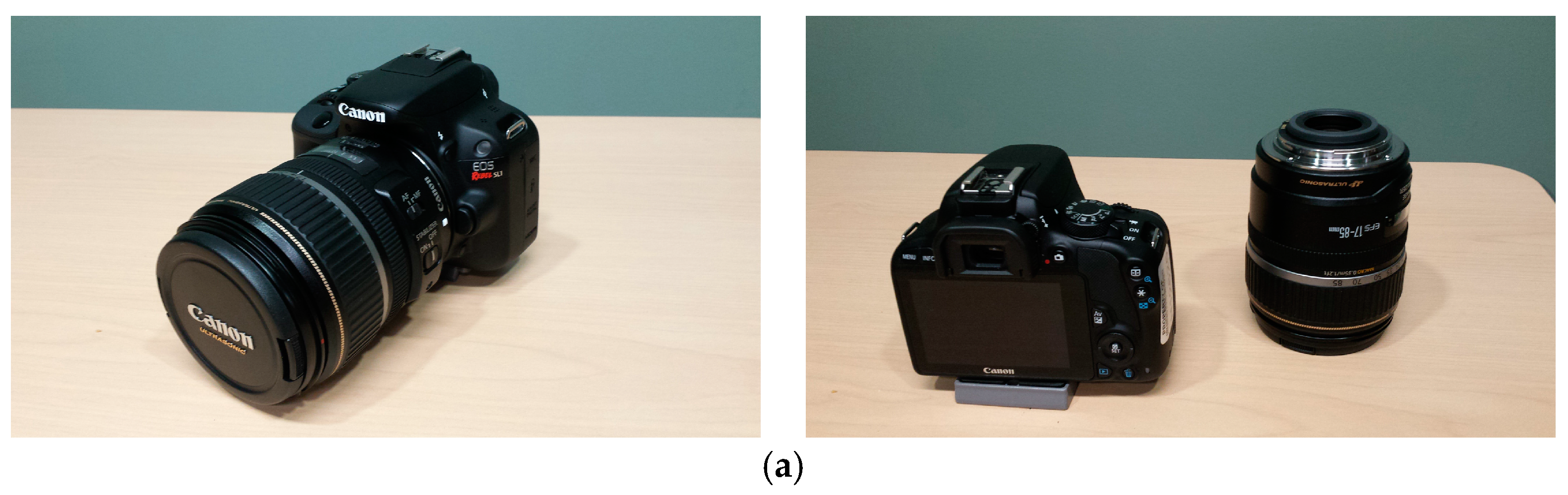

Figure 2.
3D plant model reconstruction pipeline: (a) Sample of the captured image from different view angles of an Arabidopsis plant; (b) Segmented plant objects based on the PlantCV (Plant Computer Vision) platform; (c) Reconstructed 3D model using structure from motion method; and, (d) Snapshots of reconstructed 3D model.

Figure 3.
Pseudo code for the object segmentation based on the PlantCV (Plant Computer Vision) suite.
Figure 3.
Pseudo code for the object segmentation based on the PlantCV (Plant Computer Vision) suite.
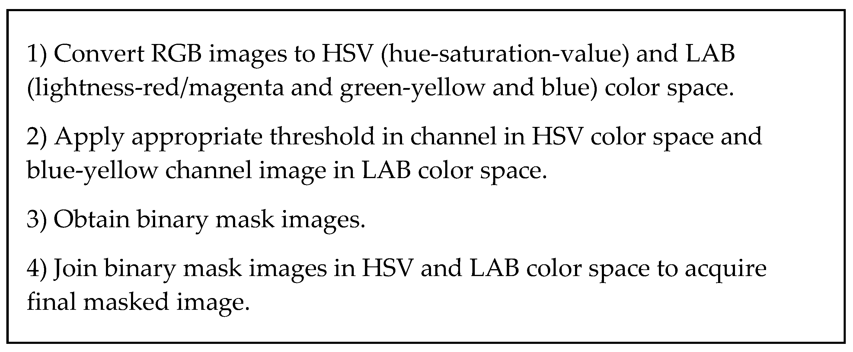
Figure 4.
Camera geometrical model.
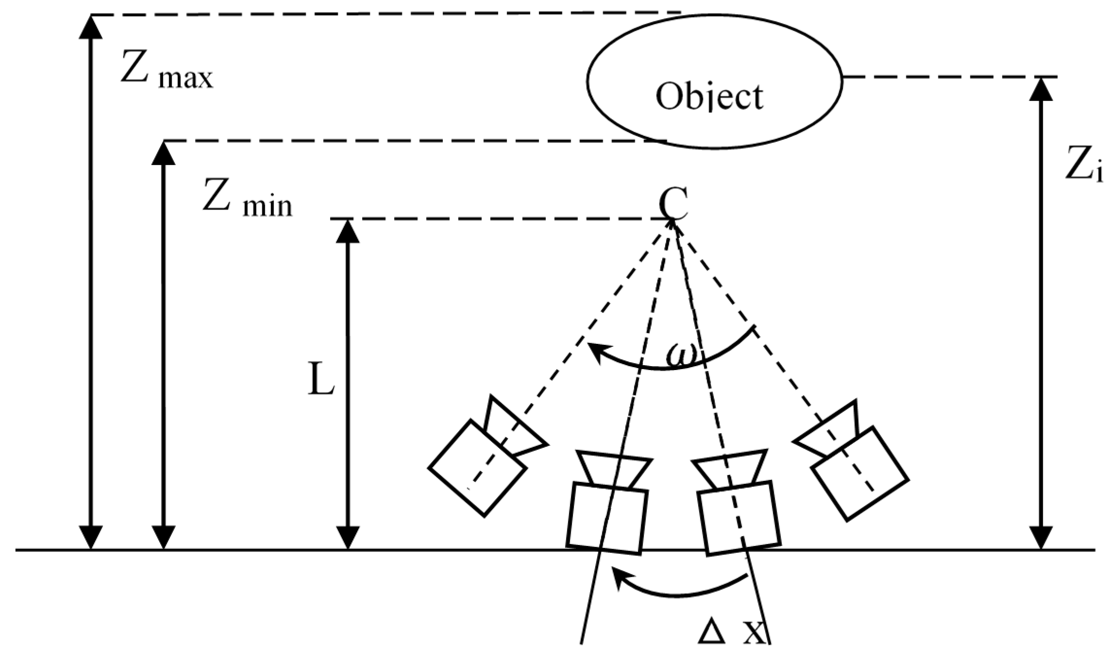
Figure 5.
3D scene capturing device: (a) Capturing camera and rotation stand; (b) Sample of the captured images with multiple view angles.
Figure 5.
3D scene capturing device: (a) Capturing camera and rotation stand; (b) Sample of the captured images with multiple view angles.
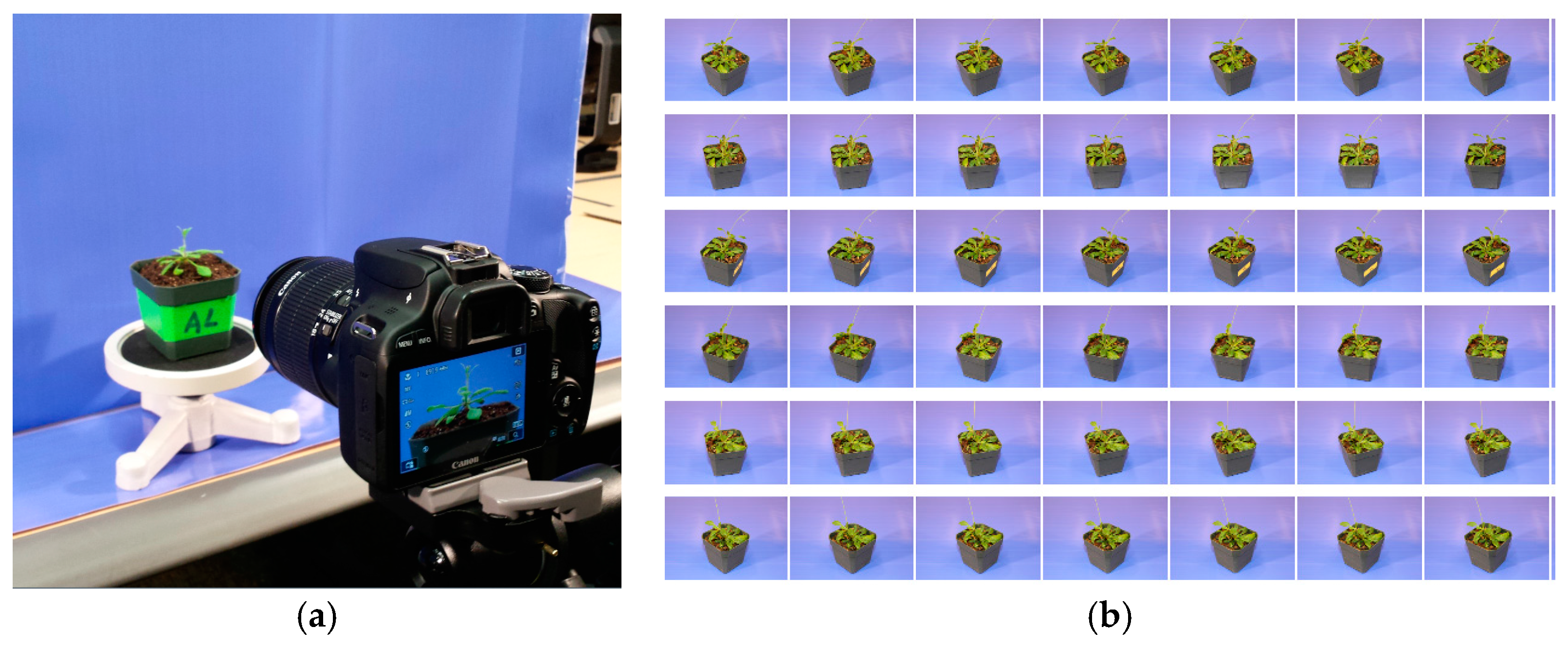
Figure 6.
Initial experiment without plant objects segmentation: (a) Capturing camera and rotation stand; (b) 3D model reconstruction based on images without segmentation; and, (c) 3D model result.
Figure 6.
Initial experiment without plant objects segmentation: (a) Capturing camera and rotation stand; (b) 3D model reconstruction based on images without segmentation; and, (c) 3D model result.

Figure 7.
Plant object segmentation method based on PlantCV.

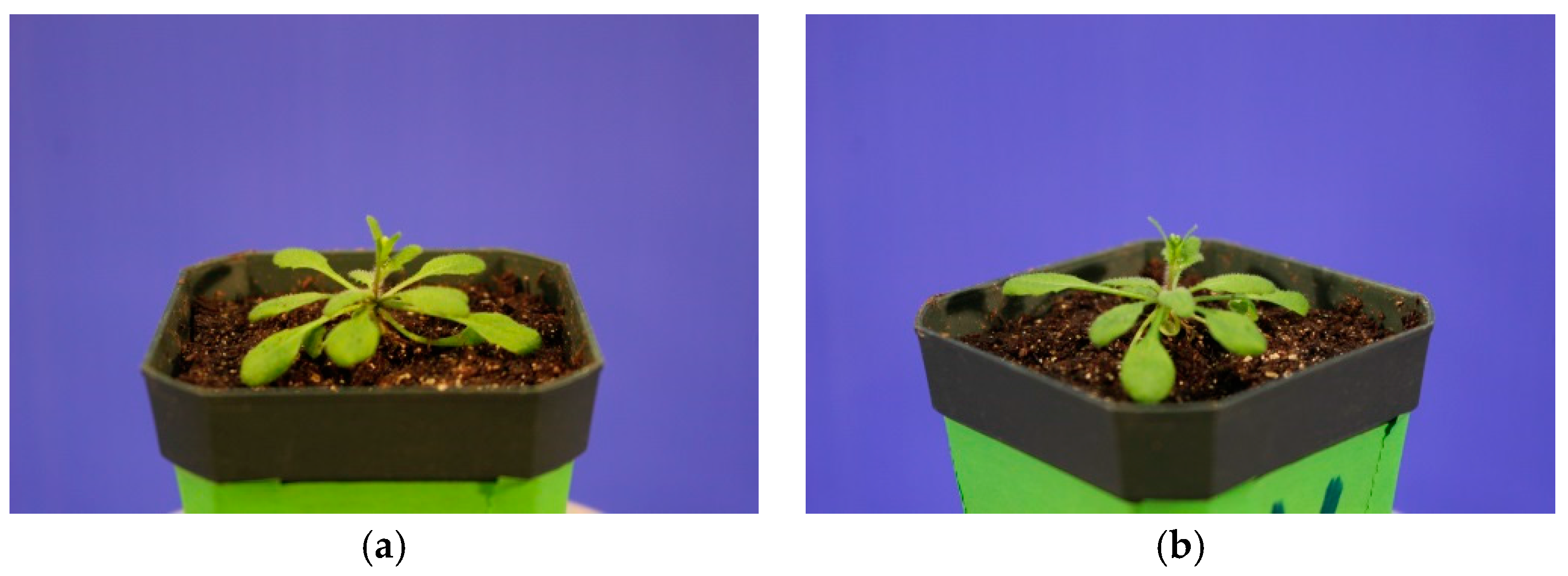
Figure 8.
Sample of the plant object segmentation results: (a,b) Sample of the captured image from different view angles of Arabidopsis plant; (c,d) Segmented plant objects based on PlantCV.
Figure 8.
Sample of the plant object segmentation results: (a,b) Sample of the captured image from different view angles of Arabidopsis plant; (c,d) Segmented plant objects based on PlantCV.

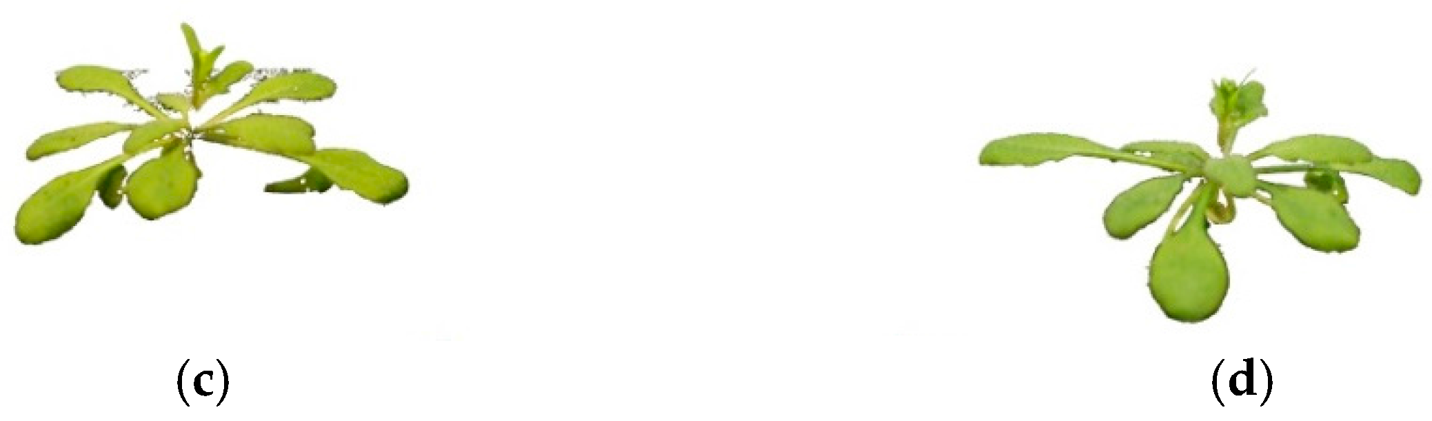
Figure 9.
High quality 3D plant model with detailed overlapping leaves.

Table 1.
Comparison of current sensors for three-dimensional (3D) reconstruction hardware systems.
| System | Principle | Advantage | Disadvantage |
|---|---|---|---|
| LIDAR (Light Detection and Ranging) | The system measures distance to a plant by illuminating that plant with a laser light. |
|
|
| Laser light system | The system projects a shifted laser on the plant. It measures distance using the reflection time. |
|
|
| Structured light system | Multiple lines or defined light patterns are projected onto the plant. It measures distance by the shift of the pattern. |
|
|
| Stereo-vision system | The system uses two cameras, which are mounted next to each other [ 5,6,7,8,9]. |
| |
| Space carving system | The same plant is imaged from multiple angles. The system uses multi-view 3D reconstruction algorithm. |
|
|
| Light field camera system | The system use conventional CCD cameras in combination with micro lenses to measure the position, intensity and origin of the incoming light. |
|
|
| Time of Flight (ToF) cameras system | The system measures the light signal between the camera and the subject for each point of the image. |
|
|
| RGB-D cameras | The system measures RGB color information with per pixel depth information. |
|
|
Table 2.
Camera parameters.
| Image Type | Width, Height | Exposure Time | Aperture Value | ISO Speed | Flash Fired | Metering Mode | Focal Length |
|---|---|---|---|---|---|---|---|
| JPEG | 3456 × 2304 | 1/60 s | 4.00 EV(f/5.6) | 500 | fired | Pattern | 50.0 mm |
Table 3.
Parameters for calculate optimal number of images.
| Zmin | Zmax | Focal Length | Pixel Pitch | Captuing Angle |
|---|---|---|---|---|
| 0.15 m | 0.45 m | 50.0 mm | 320 µm | 2 × π (rad) |
© 2017 by the authors. Licensee MDPI, Basel, Switzerland. This article is an open access article distributed under the terms and conditions of the Creative Commons Attribution (CC BY) license (http://creativecommons.org/licenses/by/4.0/).
Share and Cite
MDPI and ACS Style
Liu, S.; Acosta-Gamboa, L.M.; Huang, X.; Lorence, A. Novel Low Cost 3D Surface Model Reconstruction System for Plant Phenotyping. J. Imaging 2017, 3, 39. https://doi.org/10.3390/jimaging3030039
AMA Style
Liu S, Acosta-Gamboa LM, Huang X, Lorence A. Novel Low Cost 3D Surface Model Reconstruction System for Plant Phenotyping. Journal of Imaging. 2017; 3(3):39. https://doi.org/10.3390/jimaging3030039
Chicago/Turabian StyleLiu, Suxing, Lucia M. Acosta-Gamboa, Xiuzhen Huang, and Argelia Lorence. 2017. "Novel Low Cost 3D Surface Model Reconstruction System for Plant Phenotyping" Journal of Imaging 3, no. 3: 39. https://doi.org/10.3390/jimaging3030039
Note that from the first issue of 2016, this journal uses article numbers instead of page numbers. See further details here.