Epithelium and Stroma Identification in Histopathological Images Using Unsupervised and Semi-Supervised Superpixel-Based Segmentation ^†

Abstract

We present superpixel-based segmentation frameworks for unsupervised and semi-supervised epithelium-stroma identification in histopathological images or oropharyngeal tissue micro arrays. A superpixel segmentation algorithm is initially used to split-up the image into binary regions (superpixels) and their colour features are extracted and fed into several base clustering algorithms with various parameter initializations. Two Consensus Clustering (CC) formulations are then used: the Evidence Accumulation Clustering (EAC) and the voting-based consensus function. These combine the base clustering outcomes to obtain a more robust detection of tissue compartments than the base clustering methods on their own. For the voting-based function, a technique is introduced to generate consistent labellings across the base clustering results. The obtained CC result is then utilized to build a self-training Semi-Supervised Classification (SSC) model. Unlike supervised segmentations, which rely on large number of labelled training images, our SSC approach performs a quality segmentation while relying on few labelled samples. Experiments conducted on forty-five hand-annotated images of oropharyngeal cancer tissue microarrays show that (a) the CC algorithm generates more accurate and stable results than individual clustering algorithms; (b) the clustering performance of the voting-based function outperforms the existing EAC; and (c) the proposed SSC algorithm outperforms the supervised methods, which is trained with only a few labelled instances.

1. Introduction

Automatic segmentation of digitised histological images into regions representing different anatomical or diagnostic types is of fundamental importance for developing digital pathology diagnostic tools. Superpixel segmentation is an advanced method to group image pixels with similar colour properties into atomic regions to simplify the data in the pixel grid [1]. Recently, superpixel methods have been combined with pattern recognition techniques for image segmentation (e.g., [2]) where certain features (e.g., colour, morphology) are fed to pattern recognition procedures that assign each superpixel to expected histological classes. Supervised analysis methods are typically built from labelled training sets to predict the classes of novel unlabelled data and they require access to ‘ground truth’ reference images for the training. In contrast, unsupervised approaches (clustering analysis) do not require pre-labelled training sets for their learning but instead rely on certain similarity measures to group data into separate homogeneous clusters. In histopathological imaging analysis, clustering is of particular interest because of its potential as an exploratory tool that might provide information about hidden anatomical or functional structures in images.

Clustering algorithms use different heuristics and can be sensitive to input parameters, i.e., repeatedly applying different clustering methods on the same dataset often yields different clustering results. Furthermore, a given clustering algorithm may give rise to different results for the same data when the initialisation parameters change. Consensus Clustering (CC) [3] methods have addressed this issue by combining solutions obtained from different clustering algorithms into a single consensus solution. In unsupervised learning, this enables more accurate and robust estimation of results when compared to single clustering algorithms. CC is often performed in two steps, (a) the cluster ensemble generation, and (b) the consensus function, which finds a consensual opinion of the ensemble. CC techniques have proved to be useful in a variety of practical domains; their application to histological image segmentation is, however, relatively new.

The contributions of the proposed framework can be summarized as follows:

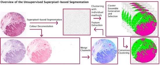
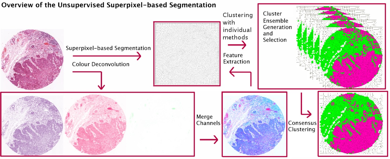
• Propose an extended version of our work in [4], in which we investigate CC in the context of superpixel-based segmentation of haematoxylin and eosin (H&E) stained histopathological images and suggest a multi-stage segmentation process.
  First, the recently proposed Simple Linear Iterative Clustering (SLIC) superpixel framework [1,5] is used to segment the image into compact regions. Colour features from each dye of H & E staining are extracted from the superpixels and used as input to multiple base clustering algorithms with various parameter initializations. The generated results (denoted here as ‘partitions’) pass through a selection scheme, which generates an ‘ensemble’ based on partitions diversity. Two consensus functions are considered here: the Evidence Accumulation Clustering (EAC) [6] and the voting-based consensus function (e.g., [7,8]).
• Suggest a new implementation for the voting-based CC method, based on image processing operations, to solve the label mismatching problem occurring among the base clustering outcomes.
  Unlike supervised methods, labels resulting from unsupervised techniques are symbolic (i.e., labels do not represent a meaningful class), and, consequently, an individual partition in the ensemble will likely include clusters that do not necessarily correspond to the labels of other clusters in different partitions of the ensemble. In the voting-based consensus function, this label mismatch is defined as the problem of finding the optimal re-labelling of a given partition with respect to a reference partition. This problem is commonly formulated as a weighted bipartite matching formulation [7,8] and it is solved by inspecting whether data patterns in two partitions share labels more frequently than with other clusters. In this paper, we present an alternative simple, yet robust, implementation for generating a consistent labelling scheme among the different partitions of the ensemble. Our approach considers the space occupied by each individual cluster in an image and exploits the fact that pairs of individual clusters from different partitions would match when their pixels overlap in a segmented image.
• Introduce a Semi-Supervised Classification (SSC) framework based on the CC method for the epithelium-stroma identification in histopathological images.
  Current supervised classification methods have reported promising results (e.g., [9,10]); however, they require large volumes of manually segmented training sets (i.e., labelled images) that are time-consuming to obtain. By contrast, our proposed unsupervised epithelium-stroma segmentation CC techniques do not require labelled data during training, but can result in a relatively lower segmentation accuracy than the supervised results. In such situations, semi-supervised learning techniques [11,12] can be of practical value as they combine the two learning strategies (supervised and unsupervised). Such approaches rely on the presence of very few labelled training instances as well as large volumes of unlabelled training samples and additionally exploit the use of unlabelled data during the learning course. Here, we propose an SSC framework based on the CC method for the epithelium-stroma identification in microscopy images. Our SSC model is based on a simple and effective semi-supervised learning methodology named the self-training method [13,14]. In this approach, a classifier repeatedly labels unlabelled training examples and retrains itself on an enlarged labelled training set. In particular, the proposed classifier is initially trained with few labelled samples and then takes advantage of the obtained CC clustering results to perform the self-training procedure. Unlike other supervised methods for epithelium and stroma segmentation, the proposed SSC approach offers an effective segmentation while relying on a small number of labelled segments. This is done by taking advantage of the knowledge acquired from clustering the unlabelled data (clustering distribution) to build a classifier that predicts the classes of unseen data (class distribution).

2. Related Work

SLIC [1] is an advanced superpixel method that generates compact and relatively uniform superpixels by agglomerating image pixels based on colour similarity and proximity in the image plane. An empirical comparison of SLIC with other state-of-the-art superpixel algorithms by Achanta et al. [5], revealing the superiority of SLIC in terms of performance and speed. They also showed that SLIC is easy to use and implement, it has low computational costs and requires fewer parameters than other algorithms, all of which are potentially useful for automatic segmentation of large, complex and variable histopathological images. SLIC superpixels have been used before to facilitate and improve unsupervised segmentation of histopathological images. For example, SLIC was applied in [2] as a pre-processing step to decrease the complexity of large histopathological images. Colour descriptors of the generated regions were then used in an unsupervised learning formulation of the probabilistic models of expected classes using the Expectation Maximisation (EM) [15]. In [16], the SLIC was exploited to enhance the segmentation of muscle fibers in muli-channel microscopy. Chen et al. [17] used the SLIC framework in a multi-label brain tumour segmentation task using structured kernel sparse representation.

Consensus Clustering (CC) methods have emerged for improving robustness, stability and accuracy of unsupervised learning solutions. Contributions in this field include the EAC [6] and voting-based algorithms. A comprehensive survey of existing clustering ensemble algorithms is presented in [3]. The voting-based methods utilize different heuristics in attempting to solve the problem of label correspondence across partitions. This is commonly formulated as a bipartite matching problem [7], where the optimal re-labelling is obtained by maximizing the agreement between the labels of an ensemble partition with respect to a reference partition. The agreement is estimated by constructing a $K\times K$ contingency table between the two partitions, where K is the number of clusters in each partition (The two partitions should contain the same number of clusters K). Each entry of the contingency table holds the number of cluster label co-occurrences counted for the same set of objects in the two partitions.

There have been previous work on CC in unsupervised histopathological segmentation, but to the best of our knowledge, its application to superpixel-based segmentation remains unexplored. Simsek et al. [18] defined a set of high-level texture descriptors of colonic tissues representing prior knowledge, and used those in a multilevel segmentation where they used a cluster ensemble to combine multiple partitioning results. Khan et al. [19] proposed ensemble clustering for pixel-level classification of tumour vs. non-tumour regions in breast cancer, where random projections of low-dimensional representations of the features and a consensus function combined various partitions to generate a final result.

The machine learning literature [11,12] has shown that engaging a large amount of unlabelled training data with a small amount of labelled training data can produce considerable improvements in learning accuracy. Such approach outperforms supervised methods trained with only few labelled training instances (which is usually insufficient for learning) as well as the unsupervised methods trained with unlabelled data alone. A successful methodology to accomplish this task is the self-training SSC. This was one of the earliest SSC methods [20] that exploited both labelled and unlabelled data in the learning process. It has successfully been applied to various real-life scenarios; however, to the best of our knowledge, its application to the problem of epithelium and stroma classification is new. Rosenberg et al. [13] applied self-training to object detection systems from images and showed that their model compares favourably against other state-of-the-art detectors. A semi-supervised self-training algorithm was proposed in [14] to segment suspicious lesions in breast Magnetic Resonance Imaging (MRI) images, where it showed superior segmentation over other popular supervised and unsupervised approaches.

3. Unsupervised Superpixel-Based Segmentation with Consensus Clustering

A block-diagram with an overview of this proposed method is presented in Figure 1.

3.1. Dataset and Preprocessing

Our data consisted of H & E stained tissue images (paraffin sections) of human oropharyngeal cancer processed into tissue micro arrays (TMAs), prepared at the Institute of Cancer and Genomic Sciences, University of Birmingham, UK. H & E is the most common staining method used in routine diagnostic microscopy; haematoxylin primarily stains nucleic acids and nuclei in blue/violet while the eosin is used as counter-stain to reveal primairly proteins in the intra- and extra-cellular compartments (in pink). TMAs are usually used for the analysis of tumour markers of multiple cases (cores) in single batches where there is a need to identify various components in the samples. Samples were digitised and background-corrected in colour using an Olympus BX50 brightfield microscope (Tokyo, Japan) with a 20× magnification objective (N.A. 0.5, resolution 0.67 $\mathsf{\mu }$m) attached to a QImaging Retiga 2000R greyscale camera (QImaging, Surrey, BC, Canada) with a tunable liquid crystal RGB filter.

Tissue core images were ≈3300 × 3300 pixels (inter-pixel distance of 0.367 $\mathsf{\mu }$m). Fifty-five images were used for the analysis (ten for training/validation and forty-five for testing), which provided the range of variation in tissue distribution typically found in this type of histological material (ranging from 2.3% to 98.8% of epithelium tissue component and 25.5% to 83.2% of background out of the whole image).

As a preprocessing step, colour deconvolution [21] was applied to the H & E image I to separate the RGB information into haematoxylin- and eosin-only images. With this procedure, up to three dyes (in our case two, H & E) can be separated into ‘stain’ channels. This procedure can be applied when the dyes on their own are known and combine subtractively, as light-absorbing materials. In the case of two-dye stains, a third component is a residual channel of the deconvolution process. The results of the colour deconvolution process can be re-combined into a “stain” false-colour RGB image here denoted $I^{*}$ (see Figure 1). In $I^{*}$, the R, G and B channels now hold the light transmittance of the haematoxylin, eosin and residual images, instead of containing the RGB components and this should retain more morphologically-relevant properties of the stained sample. The feature extraction discussed in Section 3.3 is applied to this image $I^{*}$.

3.2. Superpixel-Based Segmentation

SLIC segmentation splits-up image I into a set of superpixels held in a binary image S. The superpixels tend to be compact and relatively uniform and are formed by grouping pixels based on colour similarity and spatial proximity. In detail, a k-means algorithm [22] is used to cluster a five-dimensional vector consisting of the three components of a pixel in CIELAB colour space, plus the pixel spatial coordinates. A special similarity measure is then exploited which weighs the distance in the colour and spatial domain. This measure weighs the relative importance between color similarity and spatial proximity in the five-dimensional space. Furthermore, it allows the size and compactness of the resulting superpixels to be adjusted, providing some control over the number and shape of the superpixels generated.

In our experiments, we used the recently proposed jSLIC [23], a Java implementation of SLIC that is faster than the original (in [24]). Unlike the original, jSLIC avoids computing the same distances between data by exploiting precomputed look-up tables. Borovec et al. showed that the jSLIC is able to segment large images with intricate details into uniform parts, which is particularity useful for complexity-reduction problems (as is the case here). The authors also defined a function f that compromises between superpixel compactness and the alignment of object boundaries in the image. This is expressed as: $f=m·z^2$, where m is the initial superpixel size and z is a regularisation parameter affecting the superpixel compactness. The value of z lies within the range [0, 1], where 1 yields nearly square segments and 0 produces very “elastic” superpixels. To ensure an effective segmentation, we performed a cross validation procedure for the configuration of these two parameters, as discussed in the Experiments and Evaluation section.

3.3. Feature Extraction

Colour features are known for their relevance in visual perception and they are exploited here for the discrimination superpixels representing different histological regions. Our images contain at least three types of regions that uptake dyes differently: (a) stratified squamous epithelial tissue (a ’solid’ tissue with densely packed cells which appear darkly stained than the rest); (b) connective stroma, which is less cellular and contains abundant extracellular matrix, blood vessels, inflammatory cells, and sometimes glandular tissue; and (c) background areas, often appearing white or neutral grey.

In the feature extraction step, the colour descriptors for each superpixel in image S are computed, but, instead of referring to the original I, these are extracted from the data in image $I^{*}$ (see Figure 1), so they become “stain features” that quantify the distribution of the stain uptake in the superpixels. We used eleven measures for each stain (mode, median, average, average deviation, standard deviation, minimum, maximum, variance, skew, kurtosis and entropy) for each of the three colour deconvolution components (haematoxylin, eosin and the residual channel), forming a vector of thirty-three colour descriptors per superpixel. For the feature extraction, we used an ImageJ plugin (Particles8, Version 2.19, by G. Landini, School of Dentistry, University of Birmingham, Birmingham, UK) in [25] for estimating various statistics of binary 8-connected segmented regions.

3.4. Consensus Clustering (CC) Frameworks

The CC framework exploited here involves three main steps (a) creation of an ensemble of multiple cluster solutions; (b) selection of an effective sub-set of cluster solutions based on their diversity measure; and (c) generation of a final partition via the so-called consensus function. A clustering algorithm takes the set $X=\{x_1,x_2,\dots ,x_n\}$ of n superpixels as an input, and groups it into K clusters (epithelium, stroma and background regions) forming a data partition P. Note that $x_i$ is characterized here by the 33-dimensional colour features described in the previous section.

3.4.1. Ensemble Generation and Selection

First, a number of q clustering results are generated for the same X, forming the cluster ensemble E, where $E=\{P_1,P_2,\dots ,P_q\}$. To this end, we used five different clustering algorithms and ran each of those multiple times while varying their initialisation parameters. There are two factors that influence the performance of this approach: one is the accuracy of the individual clusters ($P_i$) and the other is the diversity within E. Accuracy is maintained by tuning a set of effective clustering methods to obtain the best set of results. Regarding the diversity of E, it was shown in [26] that a moderate level of dissimilarity among the ensemble members (E) tends to improve the consensus results. For this, we studied the diversity within E, using the Rand Index (RI) similarity measure [27], and created a more effective sub-set of cluster solutions to represent the new ensemble, denoted here as $E^{\prime }$. This new ensemble was obtained by pruning out significantly inconsistent partitions as well as identical or closely-similar partitions.

Given clustering solutions $P_i$ in the original ensemble E, in order to decide whether $P_i$ is included in $E^{\prime }$, we measure how well $P_i$ agrees with each of the clustering solutions ($P_j$) contained in E, where $i=1,\dots ,q$, as follows:

$$\begin{array}{c}\hfill \mathrm{similarity}(P_i,E)=\frac{1}{q-1}\sum _{j=1}^q\mathrm{RI}(P_i,P_j),\end{array}$$

(1)

where $(P_i,P_j\in E)$ and $(i\ne j)$. The RI counts the pairs of points (in our case superpixel pairs) on which two clusterings agree or disagree and it is computed as:

$$\begin{array}{c}\hfill \mathrm{RI}(P_i,P_j)=\frac{TP+TN}{TP+FP+TN+FN},\end{array}$$

(2)

where $TP$ and $TN$ are the number of pairs correctly grouped in the same, and different clusters, respectively. $FP$ is the number of dissimilar pairs assigned to the same cluster and $FN$ is the number of similar pairs grouped in different clusters. The RI lies between 0 and 1, where 1 implies the two partitions agreeing perfectly and 0 that they completely disagree. We defined two thresholds $T_1$ and $T_2$ that correspond to the minimum and maximum accepted levels of diversity among the partitions. If $P_i$ exhibits an acceptable level of diversity with respect to the rest of the population in E (i.e., $\mathrm{similarity}(P_i,E)\ge T_1$ and $\mathrm{similarity}(P_i,E)\le T_2$), then it is considered as an eligible voter and is added to the new ensemble $E^{\prime }$. If the opposite applies, then the partition is excluded from $E^{\prime }$. The total number of selected partitions in $E^{\prime }$ is denoted as $q^{\prime }$, where $q^{\prime }\le q$. $E^{\prime }$ is formed as follows:

$$\begin{array}{c}\hfill E^{\prime }=\{P_i|\mathrm{similarity}(P_i,E)\in [T_1,T_2]\}\end{array}$$

(3)

The next step consists of finding the consensual partition, $P^{*}$, based on the information contained in $E^{\prime }$. For this, two consensus functions are used as described below.

3.4.2. Evidence Accumulation Consensus (EAC) Function

This method, EAC-CC, considers the co-occurrences of pairs of patterns in the same cluster as votes for their association. In particular, the algorithm maps the $q^{\prime }$ partitions in $E^{\prime }$ into an $n\times n$ co-association matrix M. Each entry in M is defined as $M_{ij}=u_{ij}/q^{\prime }$, where $u_{ij}$ is the number of times the pattern pair $(i,j)$ is grouped together in the same cluster among the $q^{\prime }$ partitions. The more frequent a pair of objects appear in the same clusters, the more similar they are. Note that M is needed here because of the label correspondence problem occurring among partitions of $E^{\prime }$. M can now be viewed as a new similarity measure among the data patterns and it comprises real numbers ranging from 1 (perfect consensus among partitions) to 0 (no association). The consensus cluster $P^{*}$ is obtained by applying an appropriate similarity-based clustering algorithm on M (e.g., the hierarchical agglomerative clustering algorithm [28]). The final clustering output $P^{*}$ is represented in another image, namely $S^{\prime }$. Although the interpretation of the results of the EAC is intuitive, it has a quadratic complexity in the number of patterns, O($n^2$).

3.4.3. Voting-Based Consensus Function

This method, denoted here as Vote-CC, uses a majority voting technique to find the $P^{*}$ that optimally summarizes $E^{\prime }$. First, however, it is required to solve the problem of labelling correspondence among different partitions in $E^{\prime }$. We propose a simple re-labelling algorithm using imaging processing tools to match the symbolic cluster labels between the different partitions in $E^{\prime }$. The method finds the optimal re-labelling of a given partition P with respect to a reference fixed partition $P^{\prime }$. $P^{\prime }$ is selected from $E^{\prime }$ as the one with highest RI with respect to the ensemble (see Equation (1)).

As we are dealing with images, the procedure first assigns the labels resulting from the $P^{\prime }$ and P to the corresponding regions (or superpixels in this case) located in the binary segmented image S. The labelled regions are displayed in K unique colours in two images denoted here as $IM{G}^{\prime }$ and $IMG$ for $P^{\prime }$ and P, respectively. However, due to the label mismatching problem, a pair of correlated clusters from different partitions may be assigned different labels and the target is therefore to permute the labels, so the cluster labels in P are in the most likely agreement with the labels in $P^{\prime }$.

To this end, individual clusters displayed in images $IM{G}^{\prime }$ and $IMG$, denoted here as $k_{p^{\prime }}$ and $k_p$, are encoded in two binary images $IM{G}_{k_{p^{\prime }}}^{\prime }$ and $IM{G}_{k_p}$, respectively. Note that $k_{p^{\prime }}\in P^{\prime }$ and $k_p\in P$. The algorithm then estimates the degree of overlapping between $IM{G}_{k_{p^{\prime }}}^{\prime }$ and $IM{G}_{k_p}$ , in order to assess the similarity between the individual clusters ($k_{p^{\prime }}$ and $k_p$). The similarity is obtained using the Jaccard Index (JI) [27], defined as follows:

$$\begin{array}{c}\hfill {\mathrm{JI}}_{(IM{G}_{k_{p^{\prime }}}^{\prime },IM{G}_{k_p})}=\frac{|IM{G}_{k_{p^{\prime }}}^{\prime }\cap IM{G}_{k_p}|}{|IM{G}_{k_{p^{\prime }}}^{\prime }\cup IM{G}_{k_p}|}\end{array}$$

(4)

For every label $k_{p^{\prime }}\in P^{\prime },$ we compute ${\mathrm{JI}}_{(IM{G}_{k_{p^{\prime }}}^{\prime },IM{G}_{k_p})}$ obtained against all $k_p\in P$. Then, we find the maximum JI value that gives the most similar cluster in P to $k_{p^{\prime }}$. If $k_{p^{\prime }}$ and its highest similar $k_p$ have different labels then the matching is achieved by swapping the labels in the original image $IMG$ and therefore the labels in P. The procedure then stores the swapped labels as well as their corresponding JI in two variables. These are needed in order to track whether a label pair of ($k_p,k_{p^{\prime }}$) has already been swapped in a previous iteration. If true, then swapping $k_{p^{\prime }}$ and $k_p$ is only performed if they have higher JI value than before (i.e., the swapped pair of ($k_p,k_{p^{\prime }}$)). The process is repeated until all labels in $IMG$ have been inspected against the ones in $IM{G}^{\prime }$, and therefore clusters in P are matched with $P^{\prime }$. Note that $P^{\prime }$ remains unchanged throughout the re-labelling process. The procedure is summarized in Algorithm 1 and it has a complexity of O($K^2$). The now aligned labels for all the partitions are combined into a final consensus partition $P^{*}$ via a majority voting technique. In exceptional cases, where the number of votes are equal, we select the vote of the partitions that produce the highest total similarity (RI) with respect to the ensemble $E^{\prime }$ (Equation (1)). As before, $P^{*}$ will be represented in image $S^{\prime }$.

The idea of cluster re-labelling based on a similarity assessment has been proposed before in relation to voting-based consensus methods. However, those approaches are implemented based on inspection of the labels of data points (i.e., samples as abstract objects with no shape or size) while our re-labelling captures the similarity in a different way, based on the overlap of the superpixels, which in turn represent image regions with their own shapes and sizes.

Algorithm 1: Label Matching Algorithm for the Vote-CC Method

Input: P, $P^{\prime }$, S, n, K

Output: Labels matched for P with respect to $P^{\prime }$

for (s = 1 to n) do

Assign label of $P_s^{\prime }$ to superpixel $S_s$ and save in image $IM{G}^{\prime }$

Assign label of $P_s$ to superpixel $S_s$ and save in image $IMG$

end for

for ($k_{p^{\prime }}$ = 1 to K) do

for ($k_p$ = 1 to K) do

Threshold $k_{p^{\prime }}$ in $IM{G}^{\prime }$, convert to mask and save in $IM{G}_{k_{p^{\prime }}}^{\prime }$

Threshold $k_p$ in $IMG$, convert to mask and save in $IM{G}_{k_p}$

Compute $J{I}_{(IM{G}_{k_{p^{\prime }}}^{\prime },IM{G}_{k_p})}$ using Equation (4)

end for

$MaxJI=max\{{\mathrm{JI}}_{(IM{G}_{k_{p^{\prime }}}^{\prime },IM{G}_{k_p})},\mathrm{where}{k}_p=\{1\cdots K\}\}$

if ($k_{p^{\prime }}\ne k_p$)

SwappedLabels $=(k_{p^{\prime }},k_p)$

JISwappedLabels${}_{(k_{p^{\prime }},k_p)}=MaxJI$

if ($k_p,k_{p^{\prime }}$) ∉ SwappedLabels

Swap $k_{p^{\prime }}$ and $k_p$ and save result in $IMG$

else if (($k_p,k_{p^{\prime }}$) ∈ SwappedLabels) and (JISwappedLabels${}_{(k_{p^{\prime }},k_p)}>$ JISwappedLabels${}_{(k_p,k_{p^{\prime }})}$)

Swap $k_{p^{\prime }}$ and $k_p$ and save result in $IMG$

end If

end If

end for

Assign the new labels in $IMG$ to partition P

4. Self-Training Semi-Supervised Classification Based on Consensus Clustering

This section introduces a semi-supervised self-training classifier based on the proposed CC method (denoted here as ST-CC). The method aims at engaging large amounts of unlabelled training data, which are typically easy to obtain and abundant, with a small amount of labelled training data, that requires a high cost of labour and time to obtain. In self-training algorithms, a given classifier is trained with an initial small number of labelled samples to predict the classes of unlabelled training samples. Then, the algorithm exploits a certain hypothesis to select the most confidently predicted instance, together with their predicted labels, to be added to the labelled samples. For this, we propose using the CC results to determine the labelling confidence of unlabelled samples. The classifier is then re-trained with the new enlarged labelled samples and the process is repeated until a stopping criterion is met. The final labelled training set is used to train the classifier to predict the classes of a given test set. Note that, in the self-training method, the classifier uses its own predictions to teach itself. Furthermore, it does not impose any assumptions on the input data. The algorithm is shown in Algorithm 2 and explained in detail as follows:

Given the data set $X=x_1,x_2,\dots ,x_n$, where $x_i$ denotes a superpixel in the segmented image S, n is the total number of superpixels and each $x_i$ is characterized by the 33-dimensional colour features described earlier. The proposed ST-CC takes X as an input and splits the data instances into a training set D and a testing set T. It is assumed that T follows the same probability distribution as the given training set D. The classifier learns from D and returns the class (epithelium, stroma or background regions) of test instances in T. In the ST-CC model, the training set D is spilt into (i) labelled training instances $L=(x_1,y_1),(x_2,y_2),\dots ,(x_l,y_l)$, where $L\subseteq D$, $y_l$ are the class labels and l is the total number of labelled training instances in L, and (ii) unlabelled training instances $U=x_1,x_2,\dots ,x_u$, where $U\subseteq D$ and u is the total number of unlabelled training instances. Note that $X=D\cup T$, $D=L\cup U$, $U\gg L$ and L is randomly chosen from D using the labelled ratio ($r\%$) that is defined as follows:

$$\begin{array}{c}\hfill r\%=\frac{\mathrm{Number}\mathrm{of}\mathrm{labelled}\mathrm{instances}}{\mathrm{Number}\mathrm{of}\mathrm{all}\mathrm{the}\mathrm{instances}}=\frac{l}{n}\end{array}$$

(5)

The algorithm starts by applying the CC algorithm to U to group its instances into three different classes. The generated clustering labels are then saved in partition P. For this, we apply the Vote-CC method (proposed in Section 3.4.3) due to its lower computational complexity when compared to the EAC-CC approach. Afterwards, a supervised classifier of our choice, denoted here as h, is then trained with L to predict the labels of U that is saved in partition $P^{\prime }$. Then, the algorithm matches the clustering labels in P with the predicted class labels in $P^{\prime }$. For this, we use our re-labelling algorithm proposed in Algorithm 1, where $P^{\prime }$ is used as a reference partition to re-label the symbolic cluster labels in P. After the matching is complete, the classifier takes advantage of the consensus clustering estimated labels, which we believe to be accurate and stable, in assessing the confidence of the predicted instances in U. In particular, for each instance in U, the algorithm compares its class label (obtained by classifier h) with its clustering label (obtained by the Vote-CC). If the labels agree, then this instance is considered reliable enough to be added to the labelled training set L for a further training phases. The most confident instances are all selected and saved along with their assigned labels in a set denoted here as $U_c$, where $U_c=(x_1,y_1),(x_2,y_2),\dots ,(x_c,y_c)$ and c is the total number of reliable instances in each iteration. The new confident set $U_c$ is then added to the initial labelled training data L to form an enlarged and more robust labelled training set L, where $L=L+U_c$. $U_c$ will also be removed from U, where $U=U-U_c$. The new L will be used to retrain the given classifier h. This process is repeated until a stopping criterion is met. The criterion here measures the similarity between the predicted labels $P^{\prime }$ and the consensus clustering labels P. If the similarity is less than a defined threshold $\alpha$, then the process is repeated; otherwise, it stops and the classifier h will be trained on the final enlarged training set L to predict the classes of the test set T. The similarity here is denoted as LabelSimilarity and can be defined as follows:

$$\begin{array}{c}\hfill \mathrm{LabelSimilarity}(P,P^{\prime })=\frac{\mathrm{Number}\mathrm{of}\mathrm{samples}\mathrm{of}\mathrm{similar}\mathrm{labels}}{\mathrm{Number}\mathrm{of}\mathrm{samples}\mathrm{of}\mathrm{dissimilar}\mathrm{labels}}\end{array}$$

(6)

It was noticed that, on a few occasions after a few iterations, the similarity level reached zero, which means there are no more agreements between P and $P^{\prime }$, and therefore the similarity level can’t attain the stopping threshold $\alpha$. In this case, the process stops and the classifier h is trained on the obtained L to predict the classes of T. Note that, unlike the classical supervised methods, the proposed ST-CC makes full use of the labelled and unlabelled training samples in the learning course to come up with a robust classifier.

Algorithm 2: Semi-Supervised Self-training Classification Based on Consensus Clustering

Input: h, L, U, T, $\alpha$

Output: Predicted labels of T

Create variables P, $P^{\prime }$, $U_c$, Exit = False

Apply the Vote-CC (described in Section 3.4.3) on U and save the obtained labels in P

while (not (Exit)) do

Train h with L to predict the labels of U and save predicted labels in $P^{\prime }$

Match P with $P^{\prime }$ (reference partition) using Algorithm 1

Compute the LabelSimilarity between P and $P^{\prime }$ using Equation (6)

if (LabelSimilarity(P, $P^{\prime }$) ≤ $\alpha$) and (LabelSimilarity(P, $P^{\prime }$) ≠ 0)

for ($i=1\dots P$) do

if($P(i)=P^{\prime }(i)$) $\backslash \backslash$select the instances with confident predictions

$U_c=U_c+i$ $\backslash \backslash$add to the reliable instance i to $U_c$

end if

end for

$U=U-U_c$

$L=L+U_c$

else

Exit = True

end if

end while

Train h with L to predict the labels of T

5. Experiments and Evaluation

The purpose of the following experiments is two-fold. First, using the superpixel-based segmentation illustrates how the CC algorithms (EAC-CC, Vote-CC) improve the accuracy of clustering, compared to individual clustering approaches. Second, using the obtained Vote-CC result, the performance of the proposed ST-CC algorithm is assessed against a supervised method, both trained using a few number of true labels.

All imaging procedures and machine learning algorithms were implemented on the ImageJ platform [29] using the WEKA data mining JAVA libraries [30] running on an Intel core (TM) i7-4790 CPU (Santa Clara, CA, United States) running at 3.60 GHz, with 32 GB of RAM and 64-bit Linux operating system. All the algorithms were quantitatively evaluated by comparing their results with forty-five gold-standard H & E stained images (denoted here as R) as described earlier. A set of R images were obtained by manually labelling them into epithelium, stroma and background regions by one of us (GL) with a background in Oral Pathology.

5.1. Clustering Evaluation Methods

The effectiveness of the proposed methodology—CC applied to superpixel-based segmentation—was evaluated in the context of clustering accuracy obtained against five standard clustering approaches: (1) k-means [22]; a centroid based algorithm; (2) Unsupervised Learning Vector Quantization (LVQ) [31], an LVQ algorithm for unsupervised learning; (3) EM [15], a distribution based method; (4) Make Density Based (MDB) [32], a density based algorithm; and (5) Agglomerative Hierarchical Clustering (AH) [28], a pairwise distance based approach. These algorithms were chosen to include a range of different clustering strategies to ensure diversity in the ensemble.

We used three well-known clustering measures [27] to evaluate the algorithm results:

• The Rand Index (RI) was used to compare the final consensus clustering solution given in image $S^{\prime }$ with their corresponding reference partition given in the gold-standard image R and it is estimated as

  $$\begin{array}{c}\hfill \mathrm{RI}(S^{\prime },R)\end{array}$$

  (7)

  (see Equation (2)), where $TP$, $TN$, $FP$, or $FN$ were calculated by considering the overlapping superpixels of $S^{\prime }$ and R (as explained before).
• F1-score is defined as:

  $$\begin{array}{c}\hfill 2·\frac{Precision·Recall}{Precision+Recall}\end{array}$$

  (8)

  where

  $$\begin{array}{c}\hfill Precision=TP/(TP+FP)\end{array}$$

  (9)

  and

  $$\begin{array}{c}\hfill Recall=TP/(TP+FN)\end{array}$$

  (10)
• Jaccard Index (JI) is defined as:

  $$\begin{array}{c}\hfill \mathrm{JI}=\frac{|S^{\prime }\cap R|}{|S^{\prime }\cup R|}\end{array}$$

  (11)

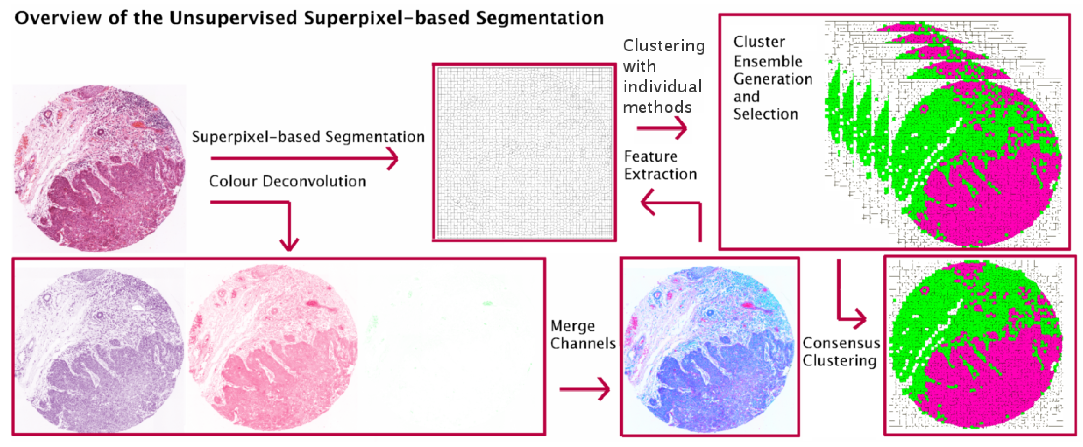
5.2. Comparing the Proposed CC with Individual Clustering Methods

In all experiments, (hyper)parameters of jSLIC and CC methods were tuned using a cross-validation procedure on a training set of ten additional images. For the superpixel segmentation, z and m were tuned over the values of (0.2, 0.3, 0.4) and (40, 50, 60), respectively. We found that the optimal values were at 0.3 and 60 for z and m, respectively. During experiments, we noticed that smaller values of z reduce the compactness of superipxels and tend to generate irregular regions, which pick up less relevant histological information from the image. In contrast, larger values of z generate more compact regions that do not adhere well to object boundaries, leading to a loss of important image information. The number of clusters was fixed to three in all experiments, corresponding to the three main types of content: epithelium, stroma and background regions. The ensemble of cluster solutions was generated by running the five aforementioned clustering algorithms multiple times with various parameter settings. The number of seeds in k-means and EM algorithms were chosen randomly from the range [10, 300]. Learning rates in the LVQ algorithm were set at the values of 0.05, 0.07, 0.09, 0.1 and 0.3. The AH algorithm was used with Complete and Mean link types. The ensemble generation process yielded a total of thirty-one clustering solutions, stored in E. The diversity selection strategy was applied to form another better performing ensemble $E^{\prime }$. For this, we assigned the values of 0.5 and 0.9 to the diversity acceptance thresholds $T_1$ and $T_2$, respectively.

Table 1. Performance evaluation of the Evidence Accumulation Consensus (EAC-CC) and Vote-CC frameworks compared against five individual clustering approaches in terms of mean Rand Index (RI), F1-score and Jaccard Index (JI) along with standard deviations (±) across the forty-five images. The best results (Vote-CC method) are marked in bold font.

Measure	EAC-CC	Vote-CC	k-Means	LVQ	EM	MDB	AH
RI (±)	0.81 ±(0.05)	0.82 ±(0.05)	0.78 ±(0.15)	0.77 ±(0.11)	0.76 ±(0.16)	0.79 ±(0.07)	0.72 ±(0.12)
F1-score (±)	0.74 ±(0.08)	0.75 ±(0.09)	0.71 ±(0.15)	0.72 ±(0.12)	0.69 ±(0.14)	0.73 ±(0.09)	0.68 ±(0.15)
JI (±)	0.71 ±(0.10)	0.72 ±(0.10)	0.69 ±(0.18)	0.61 ±(0.12)	0.66 ±(0.20)	0.68 ±(0.13)	0.60 ±(0.17)
Time(millisecond)	748.95	31.02

presents a quantitative comparison of the EAC-CC and Vote-CC methods with five individual clustering approaches (mentioned above). For each of the individual clustering algorithms, the result of the best performing run (out of the multiple runs) was selected and its mean RI, F1-score, JI and standard deviations across the forty-five images were evaluated. Figure 2 provides a visual comparison of our output against the clustering methods. For display purposes, we randomly selected one clustering output (out of the multiple runs) to represent the performance of the individual clustering approaches.

The results show that EAC-CC and Vote-CC following jSLIC segmentation produce the most accurate results out of the individual clusterings tested (81% and 82%, respectively). The accuracy of the Vote-CC comes very close to the one in EAC-CC. However, Vote-CC significantly outperformed EAC-CC in execution time. This is due to EAC-CC having a large complexity of the order O($n^2$) (in our case, n reached up to 5000 in some images) while the complexity of Vote-CC is O($K^2$) (with K = 3). The results also reveal that CC methods result in greater consistency in performance over individual clustering methods as illustrated by lower standard deviations of the RI and F1-scores. This consistency can be seen visually by comparing the results in Figure 2. In particular, despite the apparent satisfactory clustering results obtained by the single algorithms across most images, they all failed to perform well in some cases (e.g., notice the unstable performance of the LVQ, MDB and AH in the ten examples depicted in Figure 2).

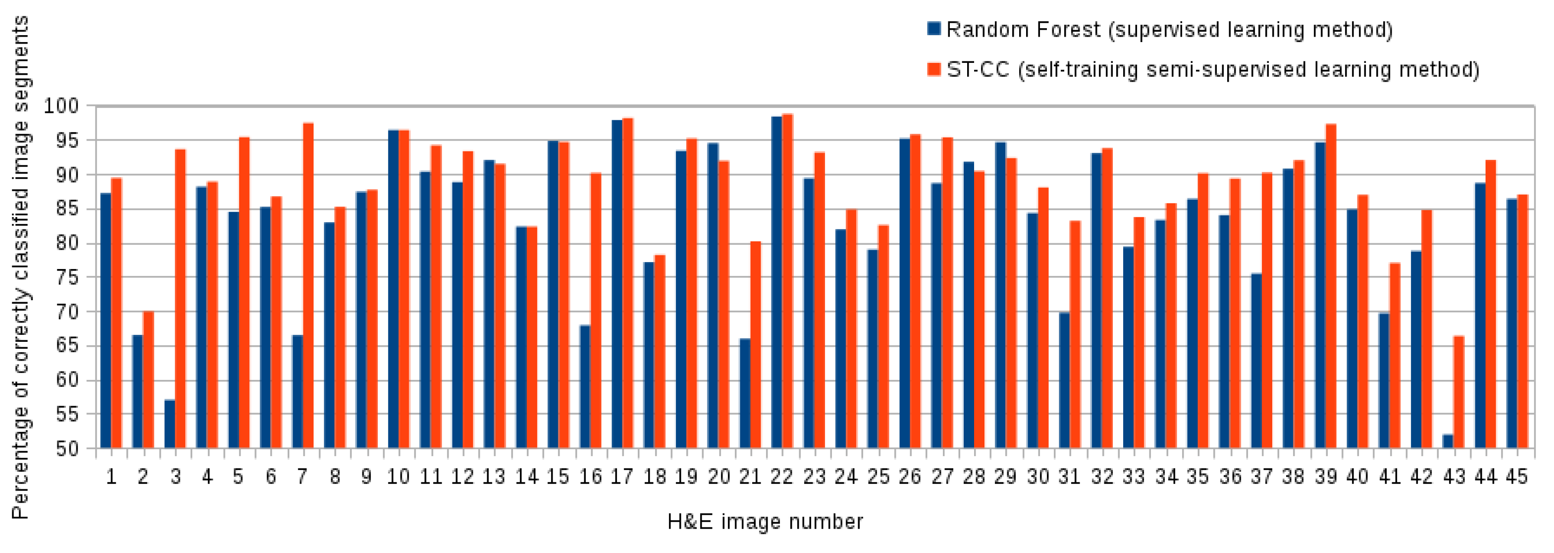
5.3. Comparing the Proposed ST-CC with Supervised Methods

The effectiveness of the proposed ST-CC framework has been evaluated in the context of epithelium-stroma classification using our forty-five H&E stained images. Specifically, we compare the classification accuracy obtained by our self-training CC-based method against a supervised method trained with only few labelled instances. In this experiment, we used the following classification accuracy measures:

• Percentage of correctly classified instances (also known as classification accuracy), the ratio between the number of test samples correctly classified to the total number of test samples.
• Precision, defined in Equation (9).
• Recall, defined in Equation (10).
• F1 score, defined in Equation (8).

Recall that each image is composed of n superpixels, where each superpixel signifies a single data item in X. For each X (image), we randomly selected 70% of data items for training D, and used the remaining 30% for testing T. The training set D was randomly split into labelled training samples L and unlabelled training samples U with percentage of 10% and 90%, respectively. This implies that r% was set to 7% (10% of the training set D, that is 70% of data), which means that 7% of the whole data set X was manually segmented. Note that, during experiments, we ensured that L included samples that represent the three classes.

To generate the clustering results in P, the Vote-CC method was applied on U with the same parameters and settings explained in the previous experiment. In order to select the best classifier to use in the ST-CC framework, the supervised model selection method in WEKA Experimenter [30] was used. The classification performance of three different classifiers (SVM [33], Random Forest [34] and J48 [35]) was tested on the 10 validation set images. The WEKA Experimenter wraps methodologies for comparing machine learning methods over multiple data sets. For each algorithm, the average classification accuracy is obtained with 10 times of 10-fold cross validation on each data set. This step revealed that the Random Forest [34] algorithm was the best classifier to use and it was well-suited for our data sets as well as the multi-class classification problem. Random forests is an ensemble learning classifier which works by constructing a multitude of decision trees at the training course and outputs the class that is the mode of the classes (classification) of the individual trees. The threshold values $\alpha$, was tuned using a cross validation procedure and set to 0.55. Recall that this threshold was used to assess the similarity between the predicted labels in $P^{\prime }$ and the anticipated labels (clustering labels) in P. To match the CC labels with the predicted labels, we used our proposed label matching technique with the same parameters used in experiment in Section 5.2.

For fair comparison, the epithelium-stroma classification accuracy of the proposed ST-CC was compared against the accuracy obtained by the Random Forest classifier, trained with L only. In particular, the average classification accuracy measures along with standard deviations (±) across the forty-five images was evaluated with the number of classes set to three in all experiments, as before.

Table 2. Performance evaluation of the self-training semi-supervised learning method (ST-CC) compared against a supervised learning approach (Random Forest classifier) in terms of Precision, Recall and F1-score along with standard deviations (±) across the forty-five images. The best results (ST-CC method) are marked in bold font.

Learning Approach	Precision	Recall	F1-Score
(self-training semi-supervised) ST-CC	0.91 ± (0.06)	0.89 ± (0.07)	0.90 ± (0.07)
(Supervised) Random Forest	0.88 ± (0.08)	0.83 ± (0.10)	0.85 ± (0.10)

illustrates the quantitative results and the highest accuracy is reported in bold font. The results show that SSTC-CC outperforms the supervised method (Random Forest), both trained with only a few labelled instances. In particular, our proposed framework produces a percentage improvement of 5.2%, 3%, 6% and 6% in classification accuracy (percentage of correctly classified instances), Precision, Recall and F1-score (respectively) when compared to the supervised method. Figure 3 compares the percentages of correctly classified points obtained by the SSTC-CC against the ones obtained by the supervised method, across the forty-five images. It is worth mentioning that the highest performance improvement reported was 37%, whereas, in a few cases (e.g., image 13 and 15), the ST-CC method didn’t achieve any performance improvement over the Random Forest classifier.

The statistical significance of the obtained classification accuracy has been assessed using the two sample (or unpaired) t-test measure. This test measures the statistical significance of the difference between two classifiers performances, one using the supervised Random Forest algorithm, and the other using our semi-supervised ST-CC method. This test produces a p-value, which can be used to decide whether there is evidence of a difference between the two population means. If the p-value is less than or equal to a predefined significance level, set here to 0.05, then the result is said to be statistically significant, and the confidence of the obtained results is confirmed. The p-value obtained here was 0.008, which is less than 0.05, which confirms that the classification accuracy result obtained here is statistically significant.

6. Discussion

Our framework offers several advantages over existing region-based methods. For instance, it is less computationally expensive than other methods such as the watershed [36] and the waterfall [37] segmentation, it helps to decrease the image spatial complexity while retaining important information about tissue compartments and it also improves the visualization and hence the interpretation of images, which are essential for automated pre-screening and guided searches on histopathological imagery.

Current supervised segmentation approaches (e.g., [38]) require the collection of large amounts of predefined labelled training images. In histopathology problems, obtaining a fully hand-labelled region annotations of images is often difficult due to the image complexity as well as the requirement of human expertise for the task. Our unsupervised approach aims to remove this burden by performing a data-independent segmentation using clustering methods. The methodology presented utilizes a consensus clustering method which allows for more robust detection of tissue regions in images when compared to individual clustering algorithms. The results obtained in Section 5.2 support this claim, showing the superiority of the CC methods (particularly the Vote-CC) over individual clusterings in terms of accuracy and stability. As illustrated in Figure 2, it is difficult to select one best clustering method that is consistently superior across all images, making it also difficult to standardise a single approach to be used across all the images.

Despite the data-independent segmentation approach of unsupervised methods (which removes the cost of labelling), they tend to exhibit lower performance with respect to supervised algorithms. This is because they cannot access the true labels in the learning process. To address this issue, we proposed a semi-supervised learning approach (the ST-CC method) in which just a small part of the training data set is labelled, leaving a large amount of training examples unlabelled. Note that even supervised classifiers often fail to produce appropriate results when only few labelled training data are available. According to our experimental results (Section 5.3), the ST-CC framework improves the segmentation accuracy, while relying on small amount of labelled regions. This might be of particular interest in problems where hand-annotated images are difficult or complicated to obtain.

One drawback of the self-training SSC method is that if an error (mis-classification) occurs during the iterative prediction of the unlabelled data, it might be reinforced (i.e., incrementally added to the original training set L), leading to low accuracy. Based on our experiments, in the self-training process, we noticed that, if L increases substantially in size, the classification accuracy starts to decline. This is believed to be due to too many labelled training instances from the clustering labels P, which may allow mistakes to reinforce themselves and therefore mislead the classifier and lead to over-fitting. This is why the growth of L (the number of instance that is added to L) was restricted by the threshold $\alpha$. It is worthwhile to mention that, on this particular issue, some procedures have been proposed (e.g., [39]) to identify and remove the mislabelled examples from the self-labelled data.

The proposed self-training algorithm appears to be a good fit model because the average accuracies obtained across the test sets in the 45 images were relatively high ( 90%) (see Table 2). This means that our model is robust enough on unseen data and its performance on the training set is close to its performance on the test set. We have used some popular techniques to prevent over-fitting and this includes a hold back validation dataset, which was used to evaluate the learned model to get a final objective idea of how the model might perform on unseen data.

Our future work concerns deeper analysis of the CC and ST-CC techniques using a larger volume of microscopy images. We aim to extend our CC method into a cluster ensemble algorithm that can determine the number of clusters k in a group of data. We also consider comparing our ST-CC to existing semi-supervised methods such as semi-supervised random forests [40].

7. Conclusions

A method of tissue segmentation of histopathological images using superpixels, Consensus Clustering (CC) and a Self-Training algorithm was presented. To the best of our knowledge, this combination has not been exploited before for microscopy image segmentation purposes. Firstly, we proposed an unsupervised method to detect regions of images that correspond to three classes of interest: epithelium, connective and background regions. A superpixel segmentation is initially performed, followed by a CC technique to combine the ‘opinions’ of several clustering algorithms into a single, more accurate and robust result using two possible approaches: EAC and the voting-based. For the latter, we introduced a label matching technique to resolve the label mismatching problem resulting from different base clustering outcomes. The algorithm proposed is easy to understand and to implement.

Secondly, we introduce a self-training semi-supervised classification method based on CC, namely ST-CC. In this method, a base classifier is trained on very few labelled samples, and then it iteratively attempts to label several unlabelled training samples that are in high agreement with the labels generated by the unsupervised CC methods. This process yields a large amount of labelled training samples that can be used for more robust prediction of tissue regions.

Experiments carried out on a set of forty-five hand-segmented H & E stained tissue images showed that the CC methods outperformed the individual clustering approaches in terms of the accuracy of the results and consistency. Furthermore, the voting-base CC using our the re-labelling technique presented here outperforms the EAC in terms of execution time. It was also shown that the proposed ST-CC outperforms supervised methods, both trained with only a few labelled training instances that are usually insufficient for learning. Compared with current supervised methods, the ST-CC overcomes the need for collecting and classifying large amounts of training data and therefore reduces human efforts of manual labelling.

References

1. Achanta, R.; Shaji, A.; Smith, K.; Lucchi, A.; Fua, P.; Susstrunk, S. SLIC Superpixels; Technical Report; École Polytechnique Fédérale de Lausanne (EPFL): Lausanne, Switzerland, 2010. [Google Scholar]
2. Borovec, J. Fully Automatic Segmentation of Stained Histological Cuts. In Proceedings of the 17th International Student Conference on Electrical Engineering, Prague, Czech Republic, 16 May 2013; pp. 1–7. [Google Scholar]
3. Vega-Pons, S.; Ruiz-Shulcloper, J. A Survey of Clustering Ensemble Algorithms. Int. J. Pattern Recognit. Artif. Intell. 2011, 25, 337–372. [Google Scholar] [CrossRef]
4. Fouad, S.; Randell, D.; Galton, A.; Mehanna, H.; Landini, G. Unsupervised Superpixel-Based Segmentation of Histopathological Images with Consensus Clustering. In Medical Image Understanding and Analysis; Valdés Hernández, M., González-Castro, V., Eds.; Springer: Edinburgh, UK, 2017; Volume 723, pp. 767–779. [Google Scholar]
5. Achanta, R.; Shaji, A.; Smith, K.; Lucchi, A.; Fua, P.; Susstrunk, S. SLIC Superpixels Compared to State-of-the-art Superpixel Methods. IEEE Trans. Pattern Anal. Mach. Intell. 2012, 34, 2274–2282. [Google Scholar] [CrossRef] [PubMed]
6. Fred, A.L.; Jain, A.K. Combining Multiple Clusterings Using Evidence Accumulation. IEEE Trans. Pattern Anal. Mach. Intell. 2005, 27, 835–850. [Google Scholar] [CrossRef] [PubMed]
7. Topchy, A.P.; Law, M.H.C.; Jain, A.K.; Fred, A.L. Analysis of Consensus Partition in Cluster Ensemble. In Proceedings of the 4th IEEE International Conference on Data Mining, Brighton, UK, 1–4 November 2004; pp. 225–232. [Google Scholar]
8. Dudoit, S.; Fridlyand, J. Bagging to Improve the Accuracy of a Clustering Procedure. Bioinformatics 2003, 19, 1090–1099. [Google Scholar] [CrossRef] [PubMed]
9. Bianconi, F.; Álvarez-Larrán, A.; Fernández, A. Discrimination Between Tumour Epithelium and Stroma Via Perception-based Features. Neurocomputing 2015, 154, 119–126. [Google Scholar] [CrossRef]
10. Linder, N.; Konsti, J.; Turkki, R.; Rahtu, E.; Lundin, M.; Nordling, S.; Haglund, C.; Ahonen, T.; Pietikäinen, M.; Lundin, J. Identification of Tumor Epithelium and Stroma in Tissue Microarrays using Texture Analysis. Diagn. Pathol. 2012, 7, 22. [Google Scholar] [CrossRef] [PubMed]
11. Chapelle, O.; Scholkopf, B.; Zien, A. Semi-supervised Learning (chapelle, o. et al., eds.; 2006) [book reviews]. IEEE Trans. Neural Netw. 2009, 20, 542. [Google Scholar] [CrossRef]
12. Zhu, X. Semi-Supervised Learning Literature Survey; University of Wisconsin-Madison: Madison, WI, USA, 2006. [Google Scholar]
13. Rosenberg, C.; Hebert, M.; Schneiderman, H. Semi-supervised Self-training of Object Detection Models. In Proceedings of the 7th IEEE Workshop on Applications of Computer Vision, Breckenridge, CO, USA, 9–11 January 2005; pp. 29–36. [Google Scholar]
14. Azmi, R.; Norozi, N.; Anbiaee, R.; Salehi, L.; Amirzadi, A. IMPST: A New Interactive Self-training Approach to Segmentation Suspicious Lesions in Breast MRI. J. Med. Signals Sens. 2011, 1, 138. [Google Scholar] [PubMed]
15. Dempster, A.P.; Laird, N.M.; Rubin, D.B. Maximum Likelihood From Incomplete Data Via the EM Algorithm. J. R. Stat. Soc. B. 1977, 39, 1–38. [Google Scholar]
16. Nguyen, B.P.; Heemskerk, H.; So, P.T.; Tucker-Kellogg, L. Superpixel-based Segmentation of Muscle Fibers in Multi-channel Microscopy. BMC Syst. Biol. 2016, 10, 124. [Google Scholar] [CrossRef] [PubMed]
17. Chen, X.; Nguyen, B.P.; Chui, C.K.; Ong, S.H. Reworking Multilabel Brain Tumor Segmentation: An Automated Framework Using Structured Kernel Sparse Representation. IEEE Syst. Man Cybern. Mag. 2017, 3, 18–22. [Google Scholar] [CrossRef]
18. Simsek, A.C.; Tosun, A.B.; Aykanat, C.; Sokmensuer, C.; Gunduz-Demir, C. Multilevel Segmentation of Histopathological Images Using Cooccurrence of Tissue Objects. IEEE Trans. Biomed. Eng. 2012, 59, 1681–1690. [Google Scholar] [CrossRef] [PubMed]
19. Khan, A.M.; El-Daly, H.; Rajpoot, N. RanPEC: Random Projections with Ensemble Clustering for Segmentation of Tumor Areas in Breast Histology Images. 2012. Available online: http://miua2012.swansea.ac.uk/uploads/Site/Programme/CS01.pdf (accessed on 9 December 2017).
20. Agrawala, A. Learning With a Probabilistic Teacher. IEEE Trans. Inf. Theory 1970, 16, 373–379. [Google Scholar] [CrossRef]
21. Ruifrok, A.C.; Johnston, D.A. Quantification of Histochemical Staining by Color Deconvolution. Anal. Quant. Cytol. Histol. 2001, 23, 291–299. [Google Scholar] [PubMed]
22. Hartigan, J.A.; Wong, M.A. Algorithm AS 136: A K-means Clustering Algorithm. J. R. Stat. Soc. Ser. C 1979, 28, 100–108. [Google Scholar] [CrossRef]
23. Borovec, J.; Kybic, J. jSLIC: Superpixels in ImageJ. Computer Vision Winter Workshop. 2014. Available online: http://hdl.handle.net/10467/60967 (accessed on 15 January 2016).
24. Borovec, J. The jSLIC-Superpixels Plugin. Available online: http://imagej.net/CMP-BIA_tools (accessed on 15 January 2016).
25. Landini, G. Advanced Shape Analysis with ImageJ. In Proceedings of the Second ImageJ User and Developer Conference, Luxembourg, 6–7 November 2008; pp. 116–121. Available online: http://www.mecourse.com/landinig/software/software.html (accessed on 1 September 2015).
26. Hadjitodorov, S.T.; Kuncheva, L.I.; Todorova, L.P. Moderate Diversity for Better Cluster Ensembles. Inf. Fusion 2006, 7, 264–275. [Google Scholar] [CrossRef]
27. Hubert, L.; Arabie, P. Comparing Partitions. J. Classif. 1985, 2, 193–218. [Google Scholar] [CrossRef]
28. Defays, D. An Efficient Algorithm for a Complete Link Method. Comput. J. 1977, 20, 364–366. [Google Scholar] [CrossRef]
29. Rasband, W.S. ImageJ.; US National Institutes of Health: Bethesda, MD, USA, 1997. Available online: http://imagej.nih.gov/ij/ (accessed on 1 September 2015).
30. Frank, E.; Hall, M.; Witten, I.H. The WEKA Workbench, 4th ed.; Morgan Kaufmann: Burlington, MA, USA, 2016. [Google Scholar]
31. Kohonen, T. Learning Vector Quantization. In The Handbook of Brain Theory and Neural Networks, 2nd ed.; MIT Press: Cambridge, MA, USA, 2003; pp. 631–634. [Google Scholar]
32. Ester, M.; Kriegel, H.P.; Sander, J.; Xu, X. A Density-based Algorithm for Discovering Clusters in Large Spatial Databases with Noise. In Proceedings of the Second International Conference on Knowledge Discovery and Data Mining, Portland, OR, USA, 2–4 August 1996; pp. 226–231. [Google Scholar]
33. Keerthi, S.S.; Shevade, S.K.; Bhattacharyya, C.; Murthy, K.R.K. Improvements to Platt’s SMO Algorithm for SVM Classifier Design. Neural Comput. 2001, 13, 637–649. [Google Scholar] [CrossRef]
34. Breiman, L. Random Forests. Mach. Learn. 2001, 45, 5–32. [Google Scholar] [CrossRef]
35. Quinlan, J.R. C4.5: Programs for Machine Learning; Elsevier: San Mateo, CA, USA, 2014. [Google Scholar]
36. Beucher, S.; Lantuéjoul, C. Use of Watersheds in Contour Detection. In International Workshop on Image Processing: Real-time Edge and Motion Detection/Estimation; BibSonomy: Rennes, France, 1979. [Google Scholar]
37. Beucher, S. Watershed, Hierarchical Segmentation and Waterfall Algorithm. In Proceedings of the Mathematical Morphology and Its Applications to Image Processing, Fontainebleau, France, 5–9 September 1994; pp. 69–76. [Google Scholar]
38. Xu, J.; Luo, X.; Wang, G.; Gilmore, H.; Madabhushi, A. A Deep Convolutional Neural Network for Segmenting and Classifying Epithelial and Stromal Regions in Histopathological Images. Neurocomputing 2016, 191, 214–223. [Google Scholar] [CrossRef] [PubMed]
39. Li, M.; Zhou, Z.H. SETRED: Self-training with Editing. In Proceedings of the PAKDD: Pacific-Asia Conference on Knowledge Discovery and Data Mining, Hanoi, Vietnam, 18–20 May 2005; pp. 611–621. [Google Scholar]
40. Leistner, C.; Saffari, A.; Santner, J.; Bischof, H. Semi-supervised random forests. In Proceedings of the 2009 IEEE 12th International Conference Computer Vision, Kyoto, Japan, 29 September–2 October 2009; pp. 506–513. [Google Scholar]
Sample Availability: The full data set with original images (tissue micro-arrays (TMA)) cannot be publicly shared due to ethical restrictions (REC Ethics Reference, 10/h1210/9). The full results of the methods described in the paper are available from the authors, School of Dentistry, University of Birmingham, Birmingham, UK.
Figure 1. Block-diagram with an overview of the unsupervised superpixel-based segmentation method.
Jimaging 03 00061 g001
Figure 2. Examples of tissue regions detection in ten haematoxylin and eosin (H&E) images—from left, the original image, gold-standard, Evidence Accumulation Consensus (EAC-CC), Vote-CC and the individual clustering methods after superpixel segmentation. Black, white, magenta and green colours correspond to the segmentation lines, background, epithelium and stroma regions, respectively.
Jimaging 03 00061 g002
Figure 3. The chart illustrates the percentage of correctly classified instances (y-axis) in each of the forty-five tested haematoxylin and eosin (H&E) images (x-axis) for the Random Forest supervised method (blue bars) and the self-training semi-supervised method (ST-CC) (red bars).
Jimaging 03 00061 g003