1. Introduction
Structural MRI can provide high resolution three-dimensional data sets of organs and tissues within the body [
1]. The images can be used to examine tissue integrity as well as to diagnose a variety of disorders [
2,
3]. The examination can be qualitative, but it can also be quantitative [
3]. The extensive quantification and analysis of the data requires further processing with automated methods such as registration and segmentation [
4]. This further processing is hampered by the presence of imaging artifacts of non-biological origin, s.a. intensity non-uniformities across an image. This artifact mainly stems from the inhomogeneity of the Radio-Frequency (RF) field due to the coil as well as due to its interaction with the subject. The inhomogeneity is more pronounced in high field MRI, which is ≥
, despite the higher contrast to noise ratio that it can potentially provide.
It is possible to calibrate for the non-uniformity of the radio-frequency field with prospective methods that involve additional acquisitions. A prospective acquisition method uses the frequency responses to parameterized acquisition sequences [
5,
6]. Another method involves the acquisition of a series of proton density weighted images in advance to estimate the inhomogeneity [
7]. The imaging of physical and geometric phantoms has also been used to approximate the combined non-uniformities of the transmission and the receiver coil(s). The physical correction methods typically involve additional acquisitions that are valid only for particular MRI sequences as well as geometries. Thus, prospective methods may not be sufficient and may reduce contrast. They also increase acquisition time that renders them more vulnerable to increased heat deposition on tissues and to motion artifacts. A general physical formulation for the complicated interaction between the radio-frequency field and the anatomy of the human body is not currently tractable.
Several retrospective restoration methods have also been proposed. They often restore individual images [
8]. Some are based on a primarily data-driven criterion and assume a distinction between lower spatial frequencies corresponding to the non-uniformities and higher ones corresponding to the anatomy. A direct implementation of this uses a low-pass homomorphic filter [
9]. In parallel imaging reconstruction, polynomial fitting of the coil data effectively performs low pass filtering that provides the respective sensitivity maps [
10]. Another primarily data-driven approach represents an image with its spatial intensity derivatives of significant magnitude that are assumed to correspond to tissues boundaries [
11,
12]. The reintegration of the normalized intensity gradients gives piecewise constant regions [
11]. Piecewise constancy has also been implemented with the Total Variation (TV) [
13]. However, the TV prior is a Laplacian distribution that is uni-modal and hence favors intensity transitions of uniform magnitude throughout an image. The regions of the same tissue that are spatially disconnected are restored independently. The spatial piecewise smoothness has also been used together with intensity clustering, s.a. fuzzy C-means, over local image windows [
14,
15,
16]. These formulations have been extended with level sets that can provide an explicit representation for two [
17] or more regions corresponding to tissues [
18].
Retrospective restoration has also been performed based on the histogram. A global histogram statistic, the entropy, has been maximized [
19]. However, the entropy is optimized for aligned mode distributions and that can be limiting [
20]. Thus, the histogram has been combined with the coring methodology [
21] that was originally developed for noise removal [
22,
23]. In the context of MRI inhomogeneity correction, coring has been combined with a spatial smoothness constraint for the field [
24,
25]. However, the histogram methods are sensitive to the level of image noise [
4,
26]. The histogram based methods can also lead to instabilities in the dynamic range and in the image domain [
19,
24,
25].
The intensity correction has been addressed together with other image analysis steps for specific applications. It has been combined with local image denoising for diffusion weighted images [
27] and with intensity standardization [
4,
28]. Intensity statistics and the histogram have also been combined with constraints for tissue classification [
14,
16]. The latter have been implemented with tissue intensity priors and with tissue spatial priors to perform simultaneously intensity restoration as well as explicit tissue segmentation [
29]. Patch-based priors have also been used for intensity correction [
30].
A patient imaging protocol typically includes multiple sequences, each of which is reconstructed independently. The resulting images can suffer from different non-uniformities. A variety of retrospective methods has been developed for their joint non-uniformity correction. A data dependent method fuses an MRI image with a Positron Emission Tomography (PET) dataset and processes the resulting image with a low-pass filter [
31]. Another data dependent method uses a variational formulation that enforces smoothness of the non-uniformity fields and also preserves the differential structure of the images [
32]. The joint restoration of two images has used the minimization of the entropy of their joint intensity histogram [
33]. A method for the simultaneous restoration of multiple co-registered images minimizes the sum of the entropies of voxelwise stack vectors over the entire image domain [
34]. The bi-contrast and multi-contrast restoration methods assume that the valid signal domains of all the images involved are identical.
A retrospective method has been developed in this study that performs a joint intensity restoration of images of two contrasts representing a certain anatomic region of a subject. In general, the retrospective methods can benefit from regularity properties of the anatomy and from the physical properties of the non-uniformities that are valid for a range of MRI contrast mechanisms and geometries. The proposed method uses the Bayesian coring methodology that involves implicit non-parametric priors. The priors are based on the auto-co-occurrence statistics for each image [
35,
36] as well as on the cross- or joint-co-occurrence statistics of the two images. The effect of the intensity distortions on the co-occurrence statistics is modeled and the statistics are restored. Additional constraints have been imposed to achieve a stable and robust restoration. These include the smoothness of the non-uniformity, the co-occurrence representation, the standardization of the dynamic ranges, and the consideration of the inevitable difference between the signal regions of the two images.
The effectiveness of the method has been demonstrated extensively with BrainWeb brain simulated images [
37]. It has also been demonstrated with brain anatomic datasets of the Human Connectome Project (HCP) (Data were provided (in part) by the Human Connectome Project, WU-Minn Consortium (Principal Investigators: David Van Essen and Kamil Ugurbil; 1U54MH091657) funded by the 16 National Institutes of Health (NIH) Institutes and Centers that support the NIH Blueprint for Neuroscience Research; and by the McDonnell Center for Systems Neuroscience at Washington University.) and with brain anatomic data sets of Parkinson’s disease patients. The performance of the method has also been compared with the performance of the N4ITK tool [
38,
39]. The comparison showed the superior performance of the proposed method. Thus, the method has been shown to improve the accuracy, the efficiency, and the stability of the restoration. It also reduces the requirements for additional acquisitions for calibration.
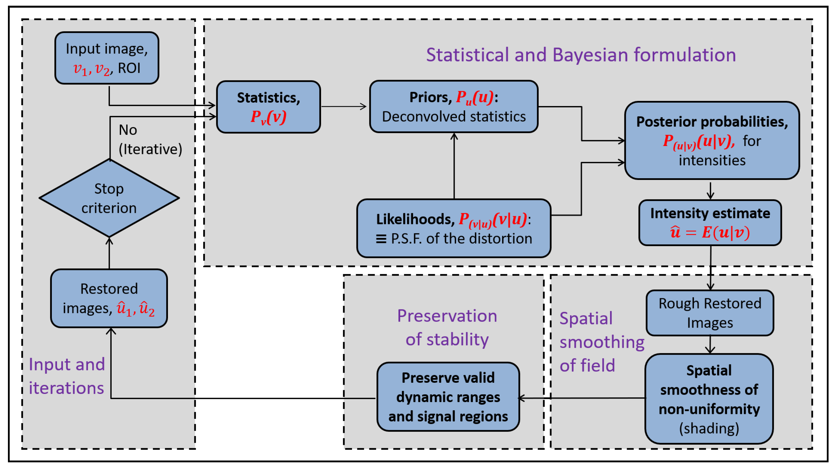
2. General Bayesian Formulation
The Bayesian formulation involves the model of the distortion that is used both directly to give the likelihood and indirectly to give the prior. In this work, the distortion is multiplicative in image domain and so the statistical distortion filter and the restoration are non-stationary. The prior is represented non-parametrically. The Bayesian estimation is repeated iteratively, t.
2.1. Spatial and Statistical Image Representation
The general formulation is introduced for a single anatomic image
, with
, which is corrupted by a multiplicative spatial intensity non-uniformity
. This is due to the combined effect of the transmit and the receive MRI radio-frequency inhomogeneities over an underlying latent anatomic image
u. The image is also corrupted with additive Rayleigh noise,
n [
40]. The noise is independent and identically distributed. That is, the images model is:
where the multiplication ∘ is the voxelwise, Hadamard product. The probability distributions of
v,
u, and
b are defined over the entire image domain. The domain is discrete and the probability distributions are computed voxelwise. The probability distributions of
and
,
and
, respectively, are assumed to be independent. It is shown in the
Appendix A that they give the probability distribution of
as:
where ∗ is the convolution. That is, the latent density of
u is convolved with a non-stationary distortion filter over the dynamic range of
u.
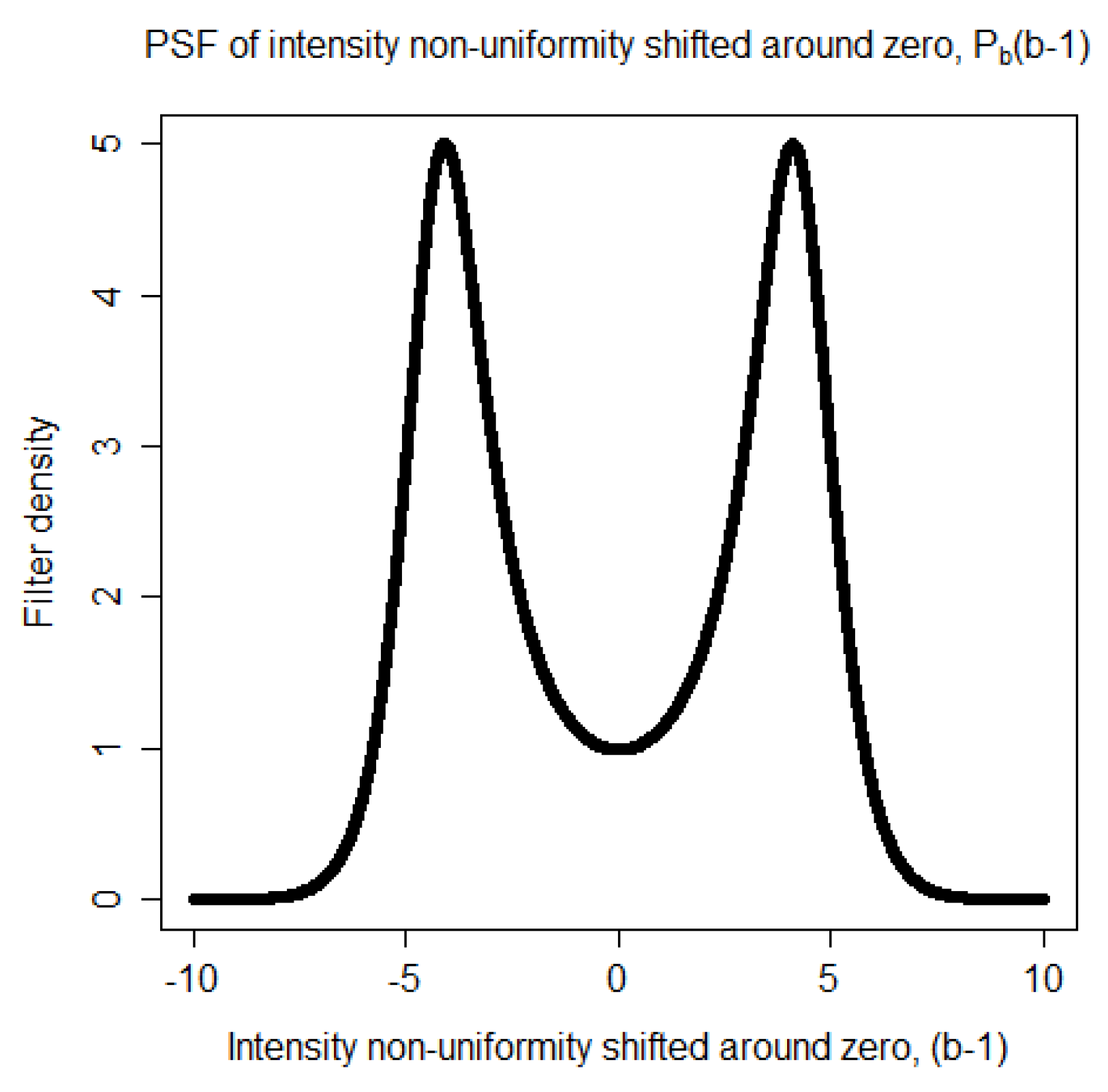
The image regions with
become brighter and the image regions with
become darker. Each of these two ranges corresponds to a mode in the distribution of the non-uniformity representing the distortion of the statistics. Thus, the Point Spread Function (PSF) of the distortion is a bimodal distribution. It is taken to be
where
is a Gaussian distribution,
is a regularization parameter, and
k is a proportionality constant. The proportionality constant
k is computed numerically so that the area of the PSF,
is equal to one. The bimodal shape of
is shown in
Figure 1.
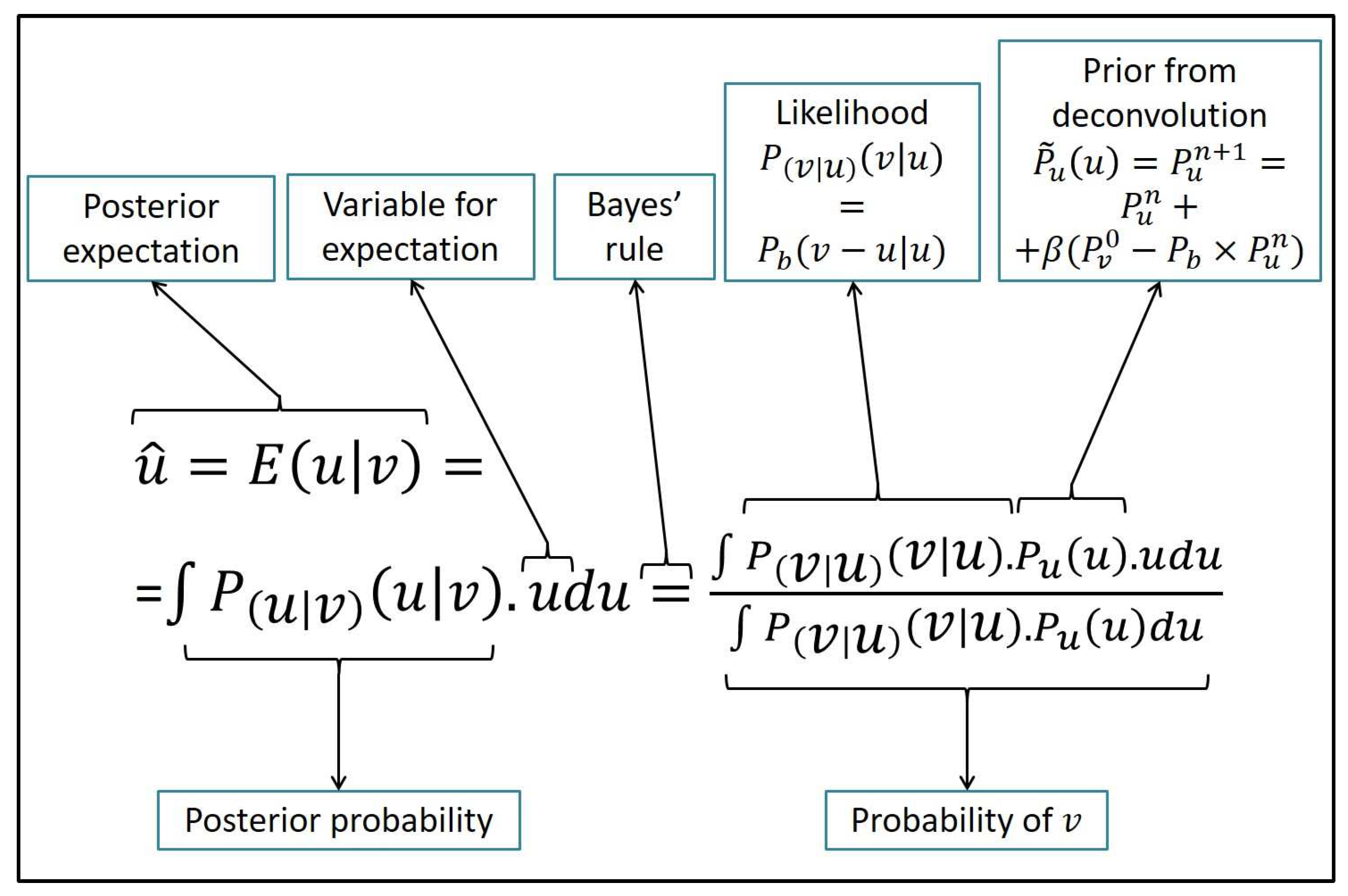
2.2. Posterior Expectation for Voxelwise Intensity Restoration
An overview of the Bayesian framework is in
Figure 2. It gives the estimate for the posterior expectation of the assumed latent intensity,
. The substitution of Bayes’ law expansion for
leads to:
This expression involves the probability distribution for latent variable u, . The latent distribution is estimated from with the deconvolution of the distortion from the actual intensity distribution . The deconvolution provides the prior as a non-parametric distribution, .
The PSF for the distortion of the intensity co-occurrences,
, increases linearly with intensity value. It is non-stationary in its direct domain that are the dynamic ranges. Thus, the deconvolution has to be non-stationary in the direct domain. The deconvolution is performed with the regularized Van Cittert method [
41,
42]. That is, the restoration is an iterative regularized algorithm formulated as
where
is the regularization constant and
is the probability of the initial image. The completion of the iterations provides the estimate
. The Van Cittert algorithm is formulated for stationary deconvolution filters. In this work, it is extended to accommodate the non-stationary PSF of
.
2.3. Back-Projection of Intensity Restoration to the Images
The restored statistics are estimated and enforced back to the image domain in a voxelwise manner. The likelihood
in Equation (
4) is equivalent to the non-stationary PSF in Equation (
2) of the intensity statistics. The prior
in Equation (
4) can be approximated by
as estimated from Equation (
5) for the co-occurrence statistics of image
u. These two terms are substituted in Equation (
4) to give
The density of
for values of
u that are far from
v tends to zero. Thus, the discretization of Equation (
6) considers only a finite neighborhood
to give:
The size of the distortion filter and of the neighborhood are non-stationary and increase linearly with intensity v.
The value of the initial restoration field,
, that is, the inverse of the distortion field, can be derived from
as it is given from Equation (
7). This is achieved with:
This provides the voxelwise restoraton expression. The restoration is iterative and the updated estimates of the restoration are used at every iteration, t. At t, the estimate of provides an updated estimate for . In turn, these two, and , provide .
The value of the restoration field for iteration
t at location
depends only on the intensity of
. Thus, the restoration can be precomputed and stored in a one-dimensional array of size equal to that of the dynamic range. It can then be indexed to expedite the back-projection of the voxelwise restoration to the image at iteration
t. The sequence of steps of the method are shown in
Figure 3. The restoration in the proposed methodology is joint for two images.
3. Methods
The Bayesian formulation is extended in various ways to represent issues related to the specific problem. An extension is for smooth spatial non-uniformities. Another extension is for the joint restoration of bi-contrast data. The identification of the signal domains of the images allows the restoration only over regions where the non-uniformity assumptions are valid. The numerical implementation of the restoration is iterative and the dynamic ranges are enforced to be stable.
3.1. Spatial and Statistical Image Representation
The method involves images of two different constrasts,
, where
. The two images are in the same anatomic space and their domains have the same spatial sampling grid. They can be corrupted by different multiplicative spatial intensity non-uniformities,
, that represent the MRI radio-frequency inhomogeneities over the underlying anatomic images
,
. Each image is also corrupted with additive Rayleigh noise,
[
40]. That is, the model becomes
and is identical for both images.
The Taylor series expansion of the non-uniformities,
, around a voxel
gives
The first order term provides a linear approximation of the non-uniformity within a spherical neighborhood
of radius
. The effects of the second and higher order terms are neglected within
. The statistical representation of images
and
is based on intensities
and
within neighborhood
. Their counts give the co-occurrence statistics as [
35,
43]:
They give the auto-co-occurrences for
and the joint-co-occurrences for
. The auto-co-occurrences are dominated by their diagonal entries and thus they are weighted down with the sigmoid
. The different tissues, or tissues interfaces, of the anatomic images
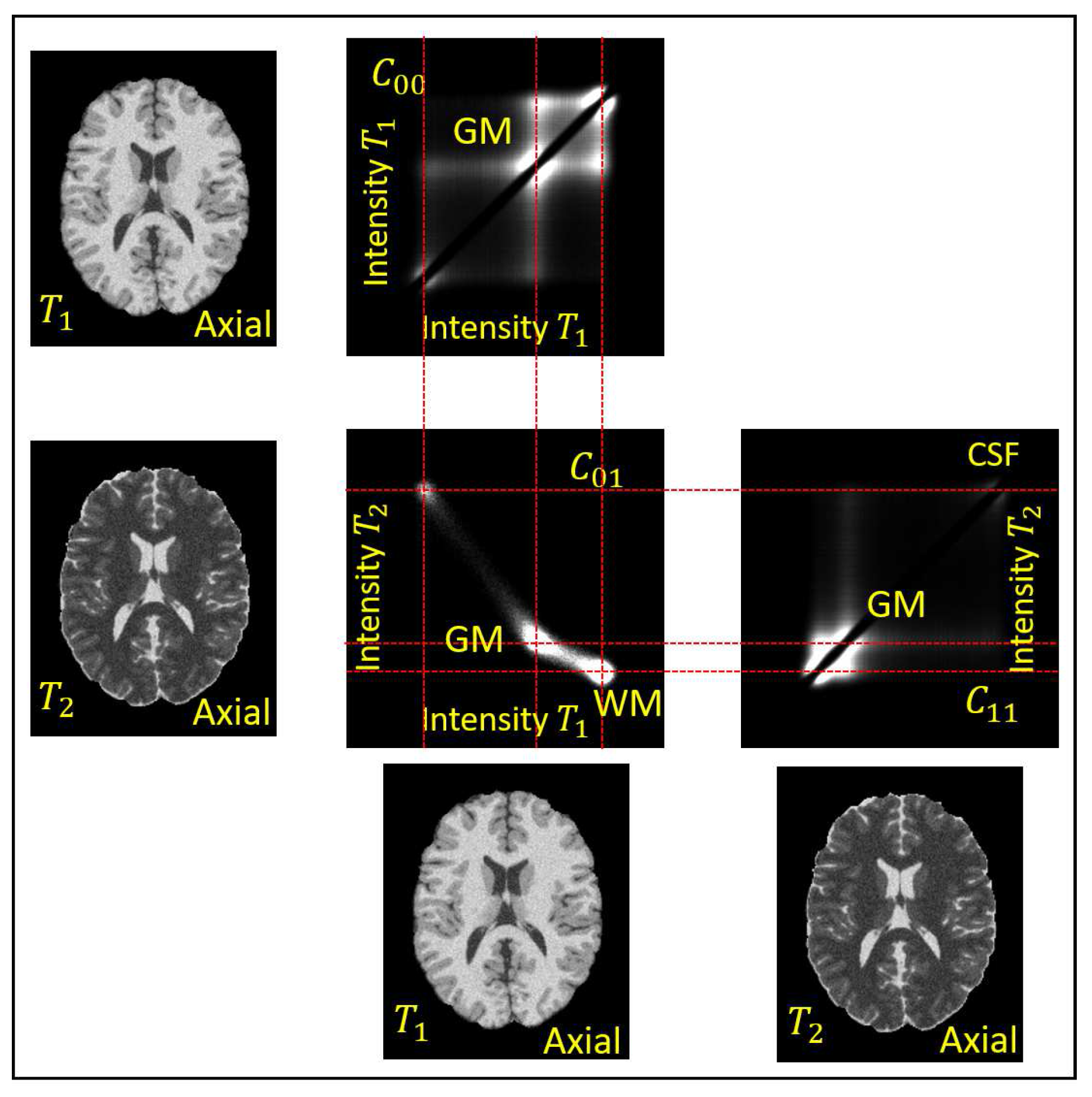
are assumed to correspond to distinct modes of the co-occurrence statistics. An example of the co-occurrences of a pair of
and
BrainWeb phantom images [
37] is in
Figure 4. A median filtering is applied to
to remove the high frequency noise
. The objective of the analysis is to separate the remaining two products in
,
present in Equation (
9) to obtain the factors
and
, respectively.
3.2. Statistical Representation of Intensity Non-Uniformities
The intensity distortions
and the latent images
are assumed to be generated by independent random variables. As shown in the
Appendix A, the statistics of the products
correspond to the convolutions of the co-occurrence statistics of the anatomic images
and
with the PSFs of the corresponding distortions. The PSFs are non-stationary to account for the multiplications in the spatial domain.
The effect of the intensity distortion field
in a neighborhood
around
can be approximated by the effect of the zero order term
and by the effect of the first order term
in Equation (
10) [
35]. The zeroth order term scales the auto-co-occurrences radially around the origin of
and the first order term rotates them around the origin. The point spread functions affecting
can be more efficiently represented in polar coordinates
. The standard deviation of the radial scaling is linearly proportional to the radial coordinate
. The standard deviation of the rotation
increases with
and is largest along the diagonal and zero along the axes. The application of the PSFs of the intensity distortions to the auto-co-occurrence statistics of the assumed underlying anatomic images
,
correspond to
. They give the convolutions
which represent the auto-co-occurrences of the distorted images.
The effects of the zero order terms of the non-uniformities
of the two images on the joint-co-occurrences
are also considered. The PSF affecting
is represented in Cartesian coordinates. Its sizes are linearly proportional to their distances from the origin
. The relation between
and
is
. The application of the PSF of the intensity distortion to the joint-co-occurrence statistics of the assumed latent anatomic images
and
that correspond to
, give
. The convolution is
and represents the joint-co-occurrence statistics of the distorted images.
3.3. Non-Stationary Restoration of the Co-Occurrence Statistics
As elaborated in
Section 3.2 and in the
Appendix A, the PSFs of the non-uniformities are non-stationary in co-occurrence space with their standard deviations being linearly proportional to the intensity coordinates. They give the convolutions in Equations (
12) and (
13). Hence, the deconvolutions of these PSF are also non-stationary. They are implemented with the non-stationary Van Cittert method in Equation (
5). The restoration of the co-occurrence statistics
,
, provide their corresponding restored estimates,
,
, respectively. The restoration of the joint co-occurrences
gives the estimate
.
3.4. Back-Projection of the Co-Occurrences Restoration to the Images
The general Equation (
7) for the case of the auto-co-occurrence statistics gives the posterior expectation of the intensities in polar coordinates in neighborhoods
and
as
where
is as given in Equation (
12). This expression for the PSF,
, also gives
from
. The posterior expectation results from separable filtering.
Equation (
7) for the case of the joint-co-occurrence statistics gives the posterior expectation of the intensities in Cartesian coordinates in neighborhoods
and
as
where
is given in Equation (
13) that also gives
from
. The conditional restoration filtering is also separable.
The general Equation (
8) provides the restoration values from the auto-co-occurrence statistics in Equation (
14) as
,
. It also provides the restoration value from the joint-co-occurrence statistics in Equation (
15) as
,
. The intensity restoration values are used to construct rectangular restoration matrices with sizes equal to the respective dynamic ranges. They are the auto-co-occurrence restoration matrices and the joint-co-occurrence restoration matrix. The repeated indexing of these matrices in an iteration expedites the back-projection of the restoration to the images.
3.5. Estimation of the Cumulative Intensity Restoration
At the first iteration,
, the restoration field is initialized with
,
, and thus, equivalently, the image is initialized with the acquired data
. At subsequent iterations, the intensity co-occurrence statistics index the corresponding auto-restoration and joint-restoration matrices to provide an initial incremental estimate of the restoration
The estimates
at iteration
t multiply the estimate of the corresponding cumulative restoration,
of the previous iteration
to give
. The estimates
are smoothed with a spatial Gaussian filter
to give the restoration fields
These are the estimates of the smoothed cumulative restoration fields. The estimates , , at iteration t, are applied to to provide that are the updated estimates of the underlying latent anatomic images.
The end condition of the iterations involves the standard deviation of , . The standard deviation decreases with iterations. The iterations stop when the value of reaches a minimum for at least one of the two images i. The field that corresponds to the iteration with the minimum value of gives which provides the restoration field . The restored images are given by . A maximum number of iterations is also imposed.
3.6. Validity of Image Domains and Stability of the Images’ Dynamic Ranges
The dynamic range of an anatomic MRI imaging sequence can be variable. The range is typically from a few hundred to a few thousand intensity levels. The dynamic range does not have a physical significance and may not even have a statistical significance. It is also affected by artifacts. In an MRI image, these can be regions of only noise, artifacts from blood flow, or artifacts resulting from tissues’ susceptibilities. The latter two can cause outlying intensities of very low or very high values.
The non-uniformity is a physical characteristic of the signal regions of an image. Thus, the dynamic range of an image is pre-processed to identify its valid sub-range for which the non-uniformity model holds. The limitation of the dynamic ranges result in distributions that are statistically meaningful. The limitation of the intensity ranges also make the filtering for deconvolution more efficient. This standardizes the dynamic ranges to normal values that correspond to the meaningful tissues contrasts intended for by the imaging sequence. It also gives the Region of Interest () in an image, . The combined of the two images is their union, . The standardization of the dynamic ranges makes the magnitudes of the distortion PSFs meaningful. The upper parts of the image dynamic ranges are downsampled linearly. The resulting complete dynamic ranges in MRI data may also be downsampled linearly.
The reference intensity to identify and standardize the valid range is the intensity value giving a high cumulative percentage, the of the dynamic range of the ROI that still corresponds to tissues. The dynamic range of the noise delimited by the maximum intensity of the noise range or minimum signal intensity, , is represented as a low fraction, , of . The minimum signal intensity for an image depends on the standard deviation of the Rayleigh noise . The dynamic range is preserved exactly up to a large upper value, of , to give . The intensity range beyond is downsampled linearly up to an intensity that corresponds to of to give the maximum intensity and the range . The intensity ranges of are back-projected to the respective images s to give the valid signal regions. The regions in image with intensities in ranges and with intensities beyond are considered invalid.
The auto-co-occurrences
in Equation (
11) and the joint-co-occurrences
are computed at least over the valid joint ranges
, for
, and for
, respectively. The same ranges are used for the Van Cittert restorations of these statistics that enable with Equation (
14) the computation of
and with Equation (
15) the computation of
. The joint restoration
also considers the complete dynamic range of the complementary image,
. The restoration gain factors in
and
that correspond to entries out of the valid intensity ranges are set to unity.
The next step is the back-projection to the images to obtain the initial estimates of the restoration fields
that use a window
in Equation (
16). The back-projection with Equation (
16) for a rough initial estimate is over the valid part of the
of image
i and is set to unity outside. The resulting estimate is smoothed as described in Equation (
17) to give
using a window depending on
. The spatial smoothing considers a weight field that is equal to one in the valid region
and is much less than one in the remaining
. As a result, the smooth non-uniformity field from Equation (
17) in regions with opposite validity in the two images tends smoothly to unity farther from the valid region and towards the invalid regions of the image with
.
The stability of the dynamic ranges along the iterations is imposed with two constraints. The first is in the spatial domain for the outputs of Equation (
16). The pixel-wise average of gains in the restoration is set to unity with the normalization
. The second constraint is in the statistics and uses the restoration field from Equation (
17). The reference intensity
along the iterations is constrained to be equal to that of the original image
. To achieve this, the final restoration fields are rescaled with
. That is, the reference intensities of
are the same as those of
.
4. Results
The method was tested with BrainWeb brain images of the phantom simulator. It was also tested with real brain datasets of the Human Connectome Project (HCP) and with images of Parkinson’s disease patients.
4.1. Implementation and Efficiency
The method was implemented in C++ as a command line program. It accepts a configuration file containing the filenames of the two images to be restored and the filenames of the images with the regions of interest that in this case are the corresponding brain masks. The program also accepts two significant command line arguments. These are the standard deviations of the size of the deconvolution filters, , and the standard deviation of the spatial smoothing filter of the restoration fields, , . The remaining parameters of the program are optional. The program was compiled with gcc (version 5.3.0). The gcc compiler was part of a Cygwin environment interfacing Microsoft Windows 10 (Microsoft, Redmond, WA, USA). The Operating System (OS) was installed and the program was executed on an Intel Core i7 processor of GHz and 64 bits. This processor has four cores and can accommodate eight threads. The processor is also combined with GB of RAM. The C++ program can be used with appropriate compilers in other OSs as well as on different processors to be converted into binary. It is thus a multi-platform implementation.
The parameters were identical for all datasets of the phantom as well as the volunteer image groups. The co-occurrence statistics are of 3D neighborhoods of size with subsampling at regular intervals along all axes. The dynamic range is limited to restrict the size of the co-occurrence matrices and the cost of their restoration filtering. The low value for the neighborhood size, , allows the setting of a low value for the angular distortion, . The first variable parameters of the method are . The parameters , are expressed as a fraction of the dynamic ranges and set to , also . The constants of the sigmoid are and . These parameters are used for the deconvolution filters with regularization . The parameters of the Van Cittert deconvolution filtering are with a total of four iterations. The second variable parameters are the standard deviations of the spatial Gaussian filters that are set to 140 pixels. The Gaussian smoothing filtering is performed separably. The iterative optimization allows using a value of that is an under-estimate and a value of that is an over-estimate in each iteration. The parameter controlling the iterations is for all datasets.
4.2. Description of the Phantom BrainWeb Brain Images
The first set was from the
BrainWeb brain MR simulator. The images were of the most commonly used anatomic brain MRI contrast mechanisms,
weighted,
w, and
weighted,
w. It consists of eight representative pairs of
w and
w images of the BrainWeb simulator [
37]. Both images in a pair have a resolution of
and a matrix of size
. They are corrupted with simulated non-uniformities of levels
b = 0% −20% −40% −60% −80% −100% and a noise of
as well as an image with
and a noise of
. Only the brain region from the entire available head region was used. The brain region of the BrainWeb images is available through the union of the tissue type classification images.
4.3. Validation Measures for the Phantom BrainWeb Brain Images
The restorations of all the BrainWeb phantom brain images were evaluated with a measure of the contrast between the intensity statistics of the gray matter and of the white matter tissues. The contrast was quantified with the Coefficient of Joint Variation (CJV) [
35,
44,
45]:
where
and
are the mean values of the two tissues intensities, and
and
are their standard deviations. This measure represents the contrast between the intensity distributions of the GM and of the WM tissue regions. The statistics and
in Equation (
18) are considered separately for each of the single contrast images
w and
w to give
and
, respectively. The ratio of the
of the restored
to the one of the corresponding original
image is also computed to give
, for
. A low value for the
is desired and thus a value for the ratio
below unity indicates effective restoration.
The BrainWeb brain phantom also makes available the original undistorted templates both for the tissue types and for the intensity values. The validation for these datasets is also performed by considering the absolute value of the difference between the restored images and the corresponding underlying undistorted templates . This difference is desired to be kept at a low value. The ratio of the difference from the restored to the difference from the original to give is also computed. It is desired to have a low value below unity for improved effectiveness.
4.4. Experiments with the Phantom BrainWeb Brain Images
The restorations of the brain part in the BrainWeb phantom images was evaluated with the intensity statistics of the GM and of the WM regions using the
given in Equation (
18). The ground truth value of the
was computed from the regions occupied by each of the two tissues available from the BrainWeb MR simulator [
37,
46]. The
was computed for the
w images to give
and for the
w images to give
. Their values are given in
Table 1. The Table shows the values for the original corrupted image pairs and the values for the intensity restored images. In parentheses is the ratio
,
. The performance of the original and of the co-occurrence restored images for non-uniformities of very low levels, 0–20%, is comparable. The improvements resulting from the restoration methods are more apparent for higher intensity non-uniformity levels. The image noise increases the
.
The difference between the corresponding original noise free and non-uniformity free phantom image and the restored ones
are also computed and shown in
Table 2. In parentheses is the ratio
,
. In all cases, its value is equal to or less than unity that shows that the restoration is effective. The duration of the restoration for a BrainWeb image pair lasts on average approximately 2 h 13 min.
The restorations of the Brainweb phantom images with noise
and with the highest level of non-uniformity,
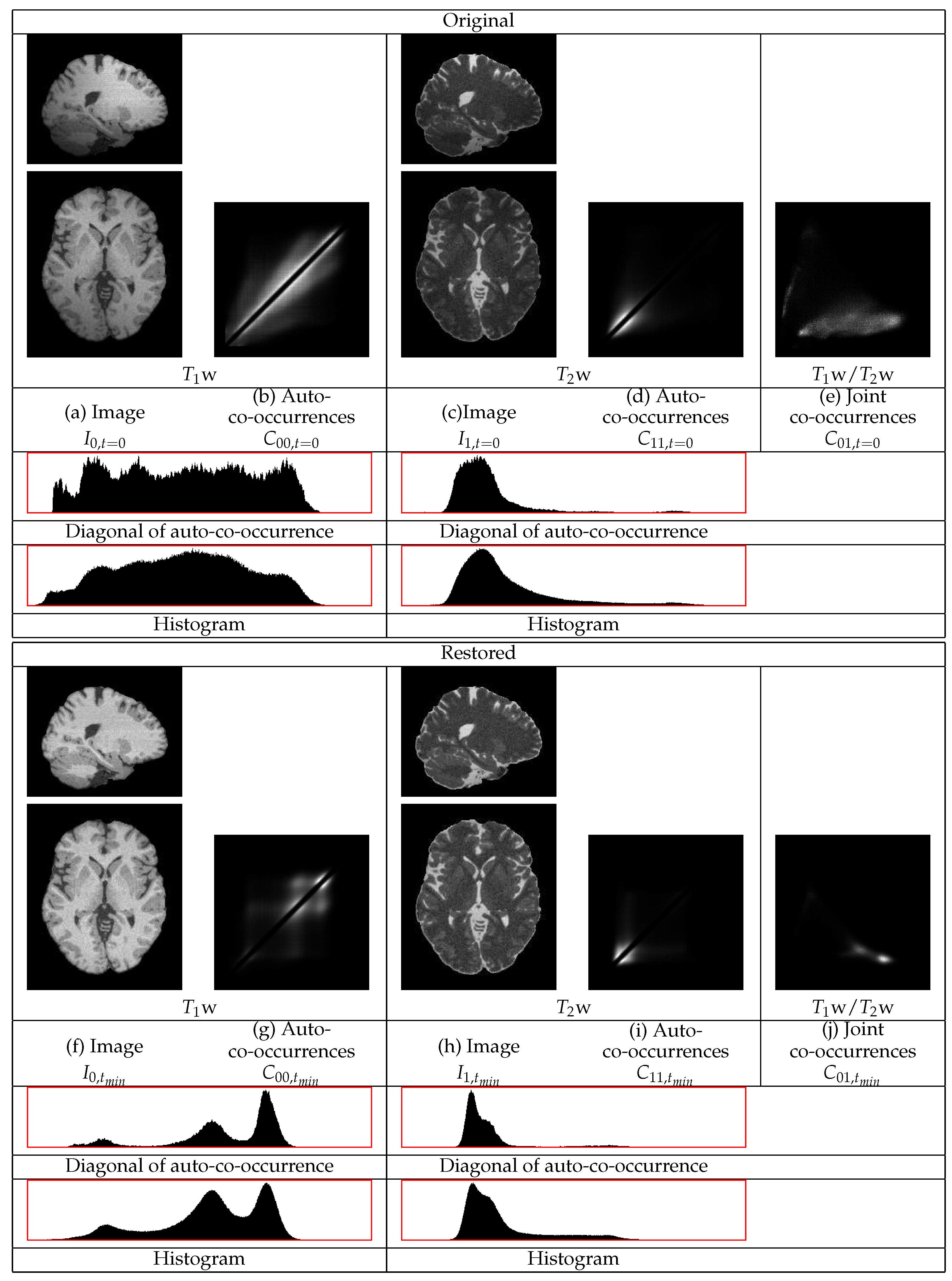
, are shown in
Figure 5. This figure contains sections from the original and from the restored images as well as the co-occurrence statistics. In this example, the cerebellum in both the
w and the
w images becomes brighter and thus its statistics become closer to those of the corresponding mean tissue statistics over the remaining image regions.
The proposed restoration method has been compared with the N4ITK tool provided through Slicer3D (version 4.6.2) [
38,
39]. The default N4ITK parameters in Slicer3D were used to restore the BrainWeb images. Similarly to the proposed method, the brain regions were provided to N4ITK. The N4ITK restoration is very weak for all images. The restoration for low levels of non-uniformity, 0–60%, leads to a significant loss of contrast for both the
weighted images and the
weighted images. This leads to an increase in the
and to
.
In high levels of non-uniformity,
and
, the restoration method with the N4ITK methodology for the
weighted images decreases contrast less based on the
. The restoration of the
w BrainWeb image with non-uniformity of
with the proposed method gives
as shown in
Table 1, whereas N4ITK gives
. That is, the performance of the proposed method is
times better than that of N4ITK. The restoration of the
weighted images also remains weak for high levels of non-uniformity. The restoration of the
w BrainWeb image with non-uniformity of
with the proposed method gives
as shown in
Table 1, whereas N4ITK gives
. That is, the performance of the proposed method for this image is
times better than that of N4ITK. Thus, the restoration of the
weighted images with the N4ITK tool performs poorly for all levels of non-uniformity. This is due to the low contrast between the distributions of the GM and of the WM in the
weighted BrainWeb images. The results based on
show a similar poor performance for N4ITK. Thus, in all cases, the proposed method performs significantly better than N4ITK.
The effects of the restoration methods on the extent of the occupied dynamic ranges of the images are also measured. The percentage of change of the size of the dynamic ranges is measured for every image restoration and for both methods. The average value over the eight images for each contrast and for each method is computed. The value of the average with the proposed method for the w images is , and, for the w images, it is . The non-zero changes are due to the noise removal from the images prior to the standardization of the dynamic ranges. The decrease is also due to the sharpening of the distributions at the high intensity parts of the dynamic ranges. The decrease for the w images is greater than for the w images. This is because, in the w images, the tissues distributions correspond to higher intensity ranges. The above values are expected and demonstrate the stability of the proposed method. The average changes in the dynamic ranges with the N4ITK tool were also measured. The average change with N4ITK for the w images is +, and, for the w images, it is . The significant positive increase in the size of the dynamic range for the w images demonstrates an instability for the N4ITK method.
4.5. Description of the Real Images
Anatomic datasets from two studies of the Human Connectome Project (HCP) [
47,
48,
49,
50] were used. The first was anatomic data from the Lifespan (LS) pilot study and the second was anatomic data from the Retest study. The data of the HCP LS study was from 27 volunteers from six age groups 4–6, 8–9, 14–15, 25–35, 45–55, and 65–75 years old. The second was data from the HCP Retest study. It was data from 45 aged volunteers, 31 women and 14 men. The volunteers were imaged at
(Siemens, Connectom and Prisma). A
weighted 3D structural MPRAGE sequence was acquired sagittally with
. A
weighted 3D structural SPACE sequence was acquired sagittally with
. The voxel resolution of both the
w and the
w images is
. The matrix size of both the
w and the
w images is
. The youngest group of age range 4–6 years old of the HCP LS pilot project was scanned using a customized pediatric head coil and an optimized protocol for that age range.
Another real dataset was of brain images of patients at an advanced stage of Parkinson’s disease. The datasets were retrieved retrospectively from the clinical database of University Hospital Goettingen for pre-operative assessment before implantation of electrodes for deep brain stimulation. The use of the patient data was retrospective, fully anonymized, and according to the guidelines of the local ethical committee for clinical research. The patients gave informed consent for all imaging procedures. All pre-operative images were acquired under anaesthesia to reduce motion artifacts and increase anatomical precision. The quality of the images was evaluated by observation and images with artifacts were removed. The data were from 60 patients, 41 men of average age years and 19 women of average age years.
The Parkinson’s disease patients were imaged at (Siemens, TrioTim). A standard weighted 3D structural MPRAGE sequence was acquired sagittally with that gave an in-plane resolution of and a slice thickness of . The matrix size of the w images is sufficient to cover the entire head region and of size at least . A high-resolution 3D SPACE structural weighted imaging that was axially planned was also acquired with that gave an in-plane resolution of and a slice thickness of . The size of the images was . In the high resolution w, the caudal cerebellum is not always depicted, depending on the skull size and “brain fitting” in a standard protocol for all Parkinson’s disease patients. The primary target in Parkinson’s disease diagnostic is the high resolution imaging of the mesencephalon and of the basal ganglia. The in-plane orientation of the two sequences are complementary to enable a more complete clinical evaluation.
The brain regions for the real images were used by the method and were extracted with the BET tool [
51]. The two brain datasets were placed in the same resolution and in the same sampling grid. The reference was the
w image and the
w image was resampled with a closest neighbor filter [
38]. The images were smoothed with a median filter of size
along the axes.
4.6. Validation Measure for the Real Brain Images
The validation measure uses the entropy of the histogram of the original image,
, and the entropy of the histogram of the restored image,
. The actual measure is the ratio
The entropies are expected values of exponents of densities of intensities. Thus, in Equation (
19), they are used as exponents of
e. A successful restoration decreases the value of the entropy of an image. Thus, both the value of the numerator in Equation (
19) and the entire ratio,
, become negative. The successful restoration also means improved tissues contrasts.
4.7. Experiments with Brain Images of the Human Connectome Project
Table 3 gives the statistics for measure
for the
w and for the
w images for all 27 volunteers of the Human Connectome Project (HCP) Lifespan (LS) dataset.
Table 4 gives the statistics for measure
for the
w and for the
w images for all 45 volunteers of the Human Connectome Project (HCP) Retest dataset. The tables show that
are indeed negative in all cases. Thus, the restorations are successful for all images. The duration of the restoration for an HCP image pair lasts on average approximately 6 h 53 min.
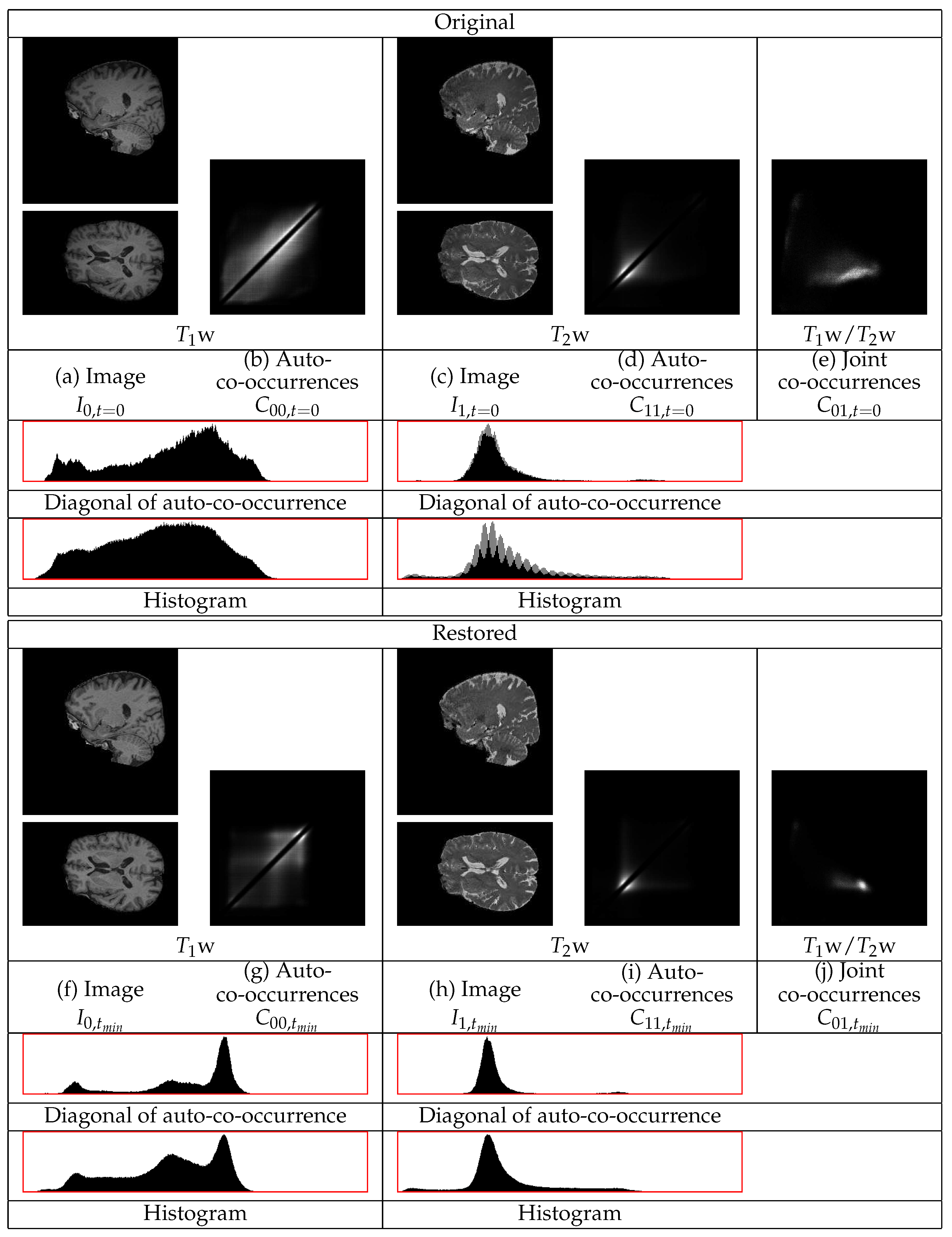
The restoration of representative
w and
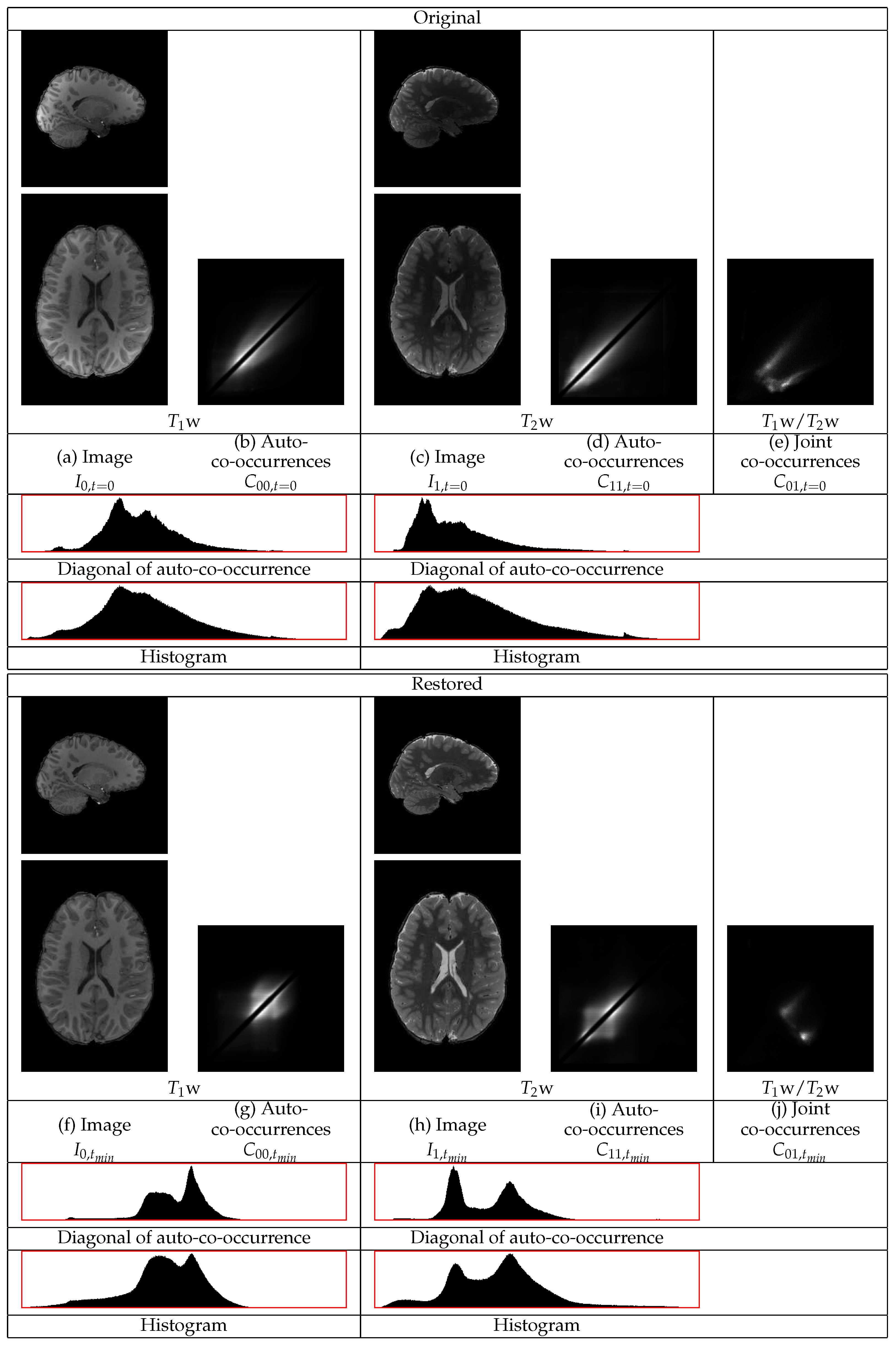
w images of an HCP volunteer are shown in
Figure 6. The GM tissues in the cortex, subcortical regions, and the cerebellum become of more uniform intensity in both images. The intensities of the WM also become more uniform. The statistics of both the
w and the
w images in
Figure 6 show different distributions corresponding to the three tissues, even along the diagonal of the auto-co-occurrences that are minimally involved in the restoration. In the
w statistics, there are separate distributions corresponding to the WM and to the GM. The distribution corresponding to the CSF appears. They also show a sharper distribution corresponding to the border between the WM and the GM. In the
w image, the different distributions of the WM and of the CSF become apparent. The consideration of both images shows their successful restoration.
The statistics of the initial w image have a heavy tail at the high intensity part of the dynamic range from contributions of the GM and of the CSF. Thus, the standardization of that part of the dynamic range to a limited range results in its compression. That compression causes a shift of densities from the lower intensity range to a higher intensity range.
4.8. Experiments with the Brain Images of Parkinson’s Disease Patients
Table 5 gives the statistics for measure
for the
w and the
w images for all 60 patients. The table shows that
is negative in all cases. Thus, the restorations are successful for all images. The duration of the restoration for an image pair of a Parkinson’s disease patient lasts on average approximately 2 h 12 min.
The restoration of representative
w and
w images with extensive non-uniformities of a Parkinson’s disease patient are shown in
Figure 7. The GM tissues in the cortex, subcortical regions, and the cerebellum become of more uniform intensity both in the
w and in the
w images. The intensity of the WM also becomes more uniform. The statistics of the
w image in
Figure 7 show three different distributions corresponding to the three tissues. The diagonal auto-co-occurrences, even though they are minimally involved in the restoration, still consist of three separate distributions. The statistics of the
w image also show distinct distributions for the WM and the GM even though they have a low contrast. They also show a sharper distribution corresponding to the border between the WM and the GM regions. The distribution corresponding to the CSF regions appears. This shows the successful restoration of the
w image. The presence of separate tissues distributions in the statistics of the restored real images gives the entropy based measure a semantic meaning in terms of tissues intensity uniformities and tissues contrasts.
The HCP LS images in
Figure 6 and the Parkinson’s disease images in
Figure 7 show that the sub-cortical regions can have a variable intensity non-uniformity effect. The restoration removes these non-uniformities. The mesencephalon and sub-cortical regions called basal ganglia and substantia nigra are implicated in Parkinson’s disease. The restoration of the uniformity in these brain regions can improve the analysis to characterize the appearance of Parkinson’s disease in MRI data [
52,
53].
5. Discussion
The Bayesian coring formulation is general and non-parametric. In this method, it is used with the auto- and the joint-co-occurrence statistics. These are higher order statistics that favor the dominant distributions of the data and decrease their spread compared to those of the intensity histogram. A sigmoid applied to the auto-co-occurrence statistics removes the dominance of their diagonal and hence increases the sensitivity to the statistics corresponding to the borders between regions. Thus, the statistics improve the discriminability between the distributions of the dominant tissues. In brain images, the extensive interface between the gray matter and the white matter tissues gives rise to one of the dominant joint distributions.
The effect of the spatial non-uniformity field on the co-occurrence statistics is modeled as a bimodal point spread function. One of the modes corresponds to multiplicative factors above unity for the regions that become brighter and the other mode corresponds to multiplicative factors below unity for the regions that become darker. The distortion filter is assumed to be non-stationary. It is used in the Bayesian formulation as both the likelihood and to compute the prior. The bimodal distribution for the distortion can be more robust to the presence of even higher field intensity non-uniformities.
The method also standardizes and preserves the valid dynamic ranges along the iterations. Thus, it offers stability and efficiency. The statistics are global over the entire ROI and this enables the uniform restoration of spatially loosely connected or even disconnected regions of the same tissue such as of the different brain gray matter centers. The method also accommodates the inevitable difference between the signal regions of the two images of different contrasts.
The restoration of MRI images for artifacts similar to the one in this work typically involve the iterative optimization of a parametric energy function. Such methods involve the computation of the histogram, its back-projection to image space, and the smoothing of the entire spatial restoration field. These steps are typically repeated in every iteration for the smoothing coefficient of each spatial basis function such as a b-spline basis. This is very intensive computationally. The method developed in this work is also iterative. However, the histogram computation and the smoothing of the entire 3D spatial field is only done once per iteration. This is significantly more efficient computationally.
The efficiency of the implementation of the methodology can be improved by taking advantage of parallelization within and between its various steps. This can be achieved by combining the C++ implementation with multi-threading. The duration of the restoration also depends on the magnitude of the non-uniformities present in the images of the pair.
The method was tested with images of the BrainWeb brain simulator. It was also tested with brain data from the Human Connectome Project (HCP) as well as data from a database of brain images of elderly patients with advanced Parkinson’s disease. Image pairs of w and w images have been restored jointly for intensity uniformity. The method restores the images successfully, despite the high intensity distortions that are present in most of them. The Parkinson’s disease patients images have a lower tissue contrast and some also contain lesions. The effectiveness of the method for this data demonstrates its efficiency. The joint restoration is mutually beneficial for both images. The proposed restoration method has been compared with the N4ITK tool. The N4ITK showed a very poor performance. The co-occurrence method performs significantly better than N4ITK. In addition, this method preserves and restores the dynamic ranges of the images. The N4ITK tool can expand the dynamic ranges of the w images that shows its instability.
A simplified model of the physical effects of the non-uniformities is assumed to design this methodology. This can lead to limitations in specific contexts. The method smooths the spatial non-uniformity field with a filter of a finite size. This allows a spatial non-uniformity of a certain magnitude. In images where the spatial non-uniformity has a lower magnitude than that of the allowed non-uniformity, the restoration may result in a loss of contrast between the tissues statistics. A complication is that the MRI physical non-uniformity also depends on the signal properties of the tissues. This is effectively ignored in this non-parametric methodology. Thus, the physical non-uniformity cannot be fully recovered [
19]. An MRI artifact that is currently ignored is the effect of the radio-frequency non-uniformity on stimulated echoes that can result in non-uniformities of the contrast, such as in the
w images. However, the restoration method in this study, as it emphasizes the intensity transitions, is more robust to the latter artifact.
The design of the methodology also makes several assumptions to improve efficiency. The restoration assumes that the removal of the noise is independent from the removal of the non-uniformity. However, the regions that become darker as a result of the restoration have lower contrast to noise ratio. Thus, the joint consideration of non-uniformity and noise may lead to an improved restoration. The method also requires the field of view for the two images to be provided. This may be more challenging for images with complicated pathology such as brain tumors. In these cases, the restoration methodology may have to be combined with other methods such as segmentation. The imaging of a brain tumor pathology may also benefit from specific imaging sequences beyond only w and w.

 ,
, 


