Hot Shoes in the Room: Authentication of Thermal Imaging for Quantitative Forensic Analysis


Bio Inspired Digital Sensing-Lab, School of Media and Communications, RMIT University, Melbourne 3000, Australia
*
Author to whom correspondence should be addressed.
J. Imaging 2018, 4(1), 21; https://doi.org/10.3390/jimaging4010021
Submission received: 31 October 2017
/
Revised: 8 January 2018
/
Accepted: 9 January 2018
/
Published: 12 January 2018
(This article belongs to the Special Issue Image Authentication Through Forensic and Watermarking Based Technologies)
Abstract
:Thermal imaging has been a mainstay of military applications and diagnostic engineering. However, there is currently no formalised procedure for the use of thermal imaging capable of standing up to judicial scrutiny. Using a scientifically sound characterisation method, we describe the cooling function of three common shoe types at an ambient room temperature of 22 °C (295 K) based on the digital output of a consumer-grade FLIR i50 thermal imager. Our method allows the reliable estimation of cooling time from pixel intensity values within a time interval of 3 to 25 min after shoes have been removed. We found a significant linear relationship between pixel intensity level and temperature. The calibration method allows the replicable determination of independent thermal cooling profiles for objects without the need for emissivity values associated with non-ideal black-body thermal radiation or system noise functions. The method has potential applications for law enforcement and forensic research, such as cross-validating statements about time spent by a person in a room. The use of thermal images can thus provide forensic scientists, law enforcement officials, and legislative bodies with an efficient and cost-effective tool for obtaining and interpreting time-based evidence.
1. Introduction
There are many examples of the use of imaging techniques to record reflected visible (400–700 nm) [1] and invisible radiation, including ultraviolet-A (UVA) (320–400 nm) [2] and near-infrared (NIR) (780–1200 nm) [3], for visualising and collecting information useful as evidence in court rooms [3,4]. However, an important consideration for the use of evidence that might be relied upon by an expert to present an opinion in a court room scenario is that such evidence should be based on well-founded and repeatable scientific principles [1,5,6]. In the case of invisible radiation, where images represent parts of the electromagnetic spectrum beyond the normal viewing experience of human court officials and jurors, it is thus especially important to have well-characterised methodologies for how such data should be interpreted in a fashion that is both reliable and repeatable [2,7,8].
The recording of various types of infrared radiation (IR) , including near, intermediate, and far wavelength, is possible through a wide range of techniques, including photographic recording of reflected NIR and thermal imaging for visualising longer wavelength infrared radiation emitted by objects heated above absolute zero (0 K) [9]. Uses of reflected infrared photographic recordings include revealing the latent marks of laser-removed tattoos for identification purposes [3,10] and pigment identification in heritage artworks [11], whilst thermal imaging can be used to assess potential damage to DNA samples on the outside of fired cartridge cases [12], observing cavitation formation by convergent–divergent constriction in pipes [13], and evaluating structural damage in heritage buildings [14].
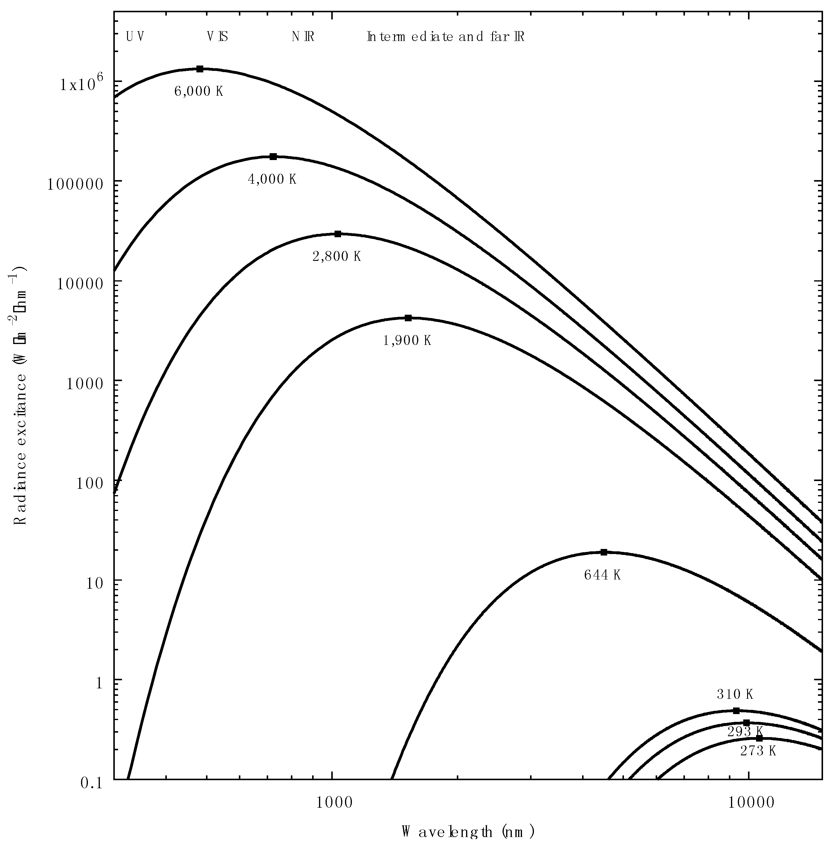
Conventional infrared photography techniques using film emulsions or modified consumer-level digital cameras are suitable to record IR radiation from about 710 up to about 900 [15] and 1100 nm [16], respectively, within the NIR (Figure 1). Beyond these wavelengths, conventional film and digital cameras are incapable of producing images representative of thermal imaging. Most commercially available thermal infrared imaging systems allow for the visualisation of radiation between 7500 to 13,000 nm, thus covering the intermediate and far IR region of the electromagnetic spectrum [17] (Figure 1). Radiation within this spectral interval would be emitted by an ideal, Planckian radiator (black body) with a temperature between about −20 °C (253 K) and 900 °C (1173 K) [18] (Figure 1). Thermal imaging sensors produce digital images where the temperature of a given area is represented by an intensity level (ρ) at each pixel location [19]. As intermediate and long infrared radiations are invisible to the unaided human eye, images produced by these devices are commonly displayed either as monochrome (grey level) or pseudo-coloured images to aid visual interpretation [20]. The output signal from a thermal imaging device is proportional to the change in temperature at each pixel site caused by the absorption of IR radiation emitted by the object being recorded [17,19,21].
The type of sensor present in a thermal imager determines the precise mechanism by which changes in temperature at a pixel site are transformed into an electric signal and subsequently transformed into a digital output [21]. The particular wavelength ranges of IR radiation that can be absorbed by a thermal imager—its spectral sensitivity—depend on the material used to construct its sensor [19]. Sensor type also determines the minimum temperature or emissivity difference that can be distinguished between two pixel sites, or thermal contrast. Contrast is also affected by digital noise, the noise equivalent temperature difference (NETD), and other sensor characteristics such as the minimum resolvable temperature difference and the minimum detectable temperature difference [19]. The term “noise” describes the random fluctuations of a signal, and encompasses a wide range of different phenomena affecting the uncertainty associated with a given digital output [16]. Sources of digital noise affecting thermal imagers include, but are not limited to, thermal, tan-δ, current, 1/f, radiation and temperature fluctuation flicker, or burst noise [21]. NETD is set by the minimal temperature difference required by a particular sensor to produce a signal response above the noise threshold, which is also determined by the minimum radiant flux detectable by an imager, the Noise-Equivalent-Power (NEP) [17,21]. Altogether, these characteristics affect the quality of the image, potentially leading to incorrect temperature readings from camera output, and, thus, an incorrect quantitative interpretation of image data.
Objects with a temperature that is above absolute zero and hotter than its surroundings cool down by transferring energy through convection, conduction, and radiation [22]. This process will continue without interruption until both the temperature of the object and the environment are at equilibrium, at which point the exchange of energy between systems is null. At this point, the temperatures between the object and its surrounding environment are equal and no further cooling of the object is observed [22]. However, the precise analytical modelling of the cooling process for real objects in nonlaboratory environments, as those commonly faced by forensic experts, is not trivial, often requiring knowledge of several parameters unique for the object under study [23]. Consequently, the development of an efficient and easily implementable method for measuring time based on the temperature of objects likely used or worn by a suspect for first responders to a potential crime scene is highly desirable.
The ability to reliably predict in field conditions the time since an object commenced cooling could be of use as a tool to validate evidentiary reports regarding the amount of time since an event of interest. For example, under certain given conditions, it would be possible to assess the amount of time since a suspect has left a crime scene, or if the amount of time spent by a suspect at a given location is likely to be true. In this research paper, we propose a method for quantitatively estimating time by using as a predictor the temperature of an object as recorded by a portable thermal imaging device in a typical house environment, without knowledge of proprietary information, to provide forensic evidence that can stand up to rigorous cross-examination in a court of law in line with contemporary guidelines for determining the reliability of evidence [5].
2. Materials and Methods
2.1. Scenario
We consider the problem of predicting the time since three different shoe types have been removed from the foot of a subject based on the pixel intensity values (ρ) of an image recorded with a portable thermal imager. This is a plausible scenario when a person of interest may have been seen probably entering a room, and may have recently removed footwear to maintain that they have not been outside of the room for an extended period. If a mobile thermal camera could precisely establish the validity of the evidence in this scenario it would facilitate efficient decision-making by law enforcement officers, or provide scientific images that could be used as evidence in court. Our experiments were carried out in typical room conditions with an ambient temperature of 21.9 °C (±0.326 SD) and humidity of 40.7% (±4.60 SD). For this experiment, we considered a male subject of 171.0 cm height and weighing about 84 kg, who was one of the authors of the study (Justin H. J. Chua). To simulate typical wearing conditions, the subject wore the shoes for 30 min, of which the final 10 min were spent walking, before commencing the measurements. Probes were fitted following the removal of the shoe, taking up to 3 min.
2.2. Experimental Shoe Types
Three different shoe models were used for the experiment, representing typical shoe types: (i) Running shoes (Asics Cumulus 12, Kobe, Japan); (ii) common leather dress shoes (Country Road, Melbourne, Australia); and (iii) trail running shoes (Asics Fuji Trabuco 5 GTX, Kobe, Japan). We considered the left shoe for all reported experimental results, after pilot experiments revealed no observable differences between left and right shoes.
2.3. Temperature and Image Recording
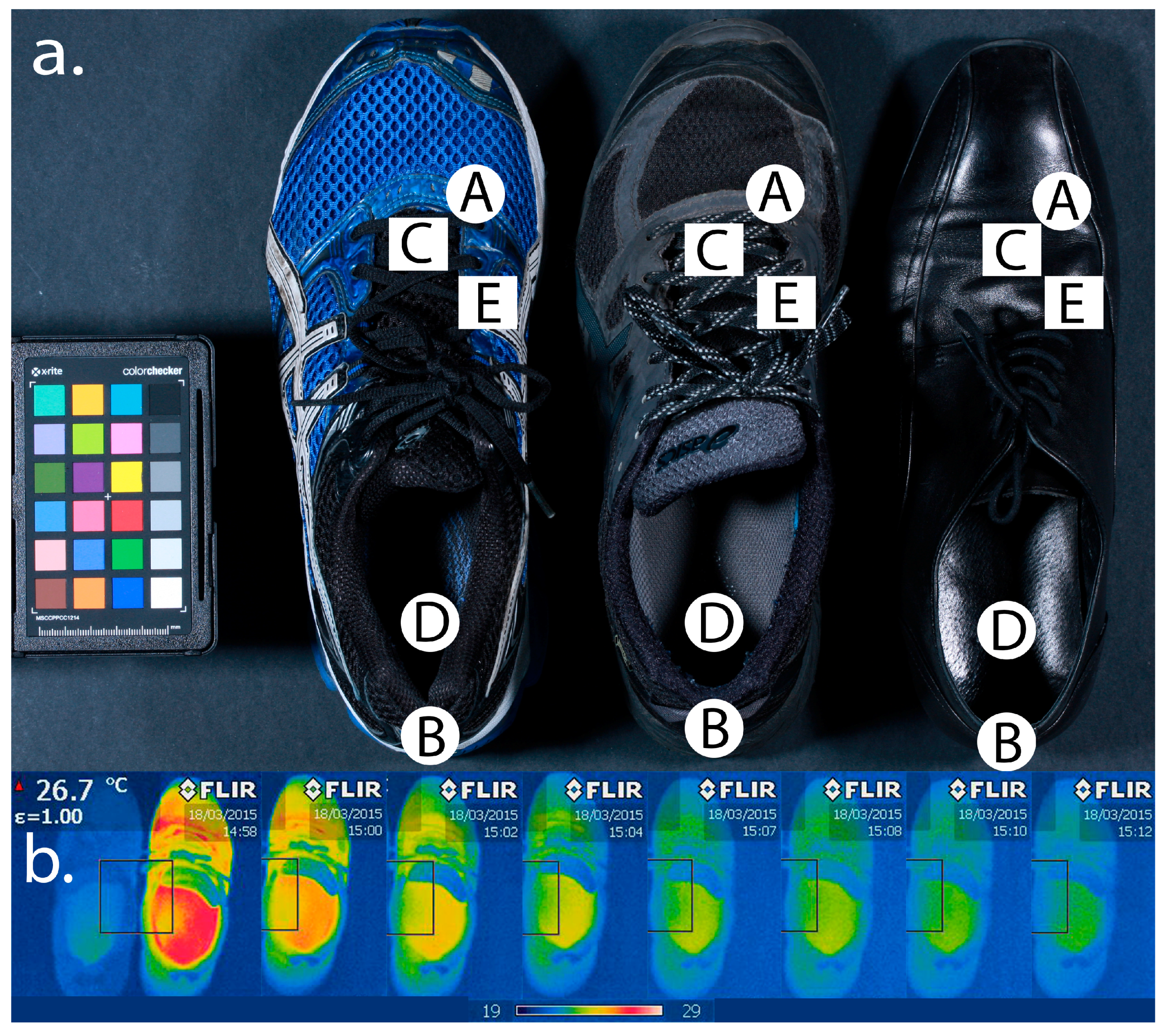
Ambient room temperature and point shoe temperature measurements were collected by an Automatic Weather Station and Thermistor Sensor, respectively, and stored in ASCII files using a modular data logging system from ICT International Pty Ltd. (Armidale, Australia). The station consists of an ICT Voltage Sensor Logger (VSL), an Automatic Weather Station, and a Therm-Micro Thermistor Sensor adapted with a Temperature Sensor Meter. Three Therm-Micro Thermistor sensors were anchored to the internal points of the shoe (points C–E in Figure 2) using a steel wire frame and tape, while external points A and B were secured with tape. The probe was insulated from the steel wire frame using plastic tubing of 6 mm diameter and weighted down with Blu-Tack (Bostik Australia Pty Ltd., Essendon Fields, Australia). The Therm-Micro sensors recorded the temperature of the external surface of the shoe over the big toe, the external surface of the heel area just next to the collar, the insole at the ball of the foot, the insole at the heel of the foot and a point on the insole closest to where the thermal imager is measuring at a targeted point (points A–E in Figure 2).
The Voltage Sensor Logger was tethered to a 64-bit Windows 10 operating system computer with an Intel® Core™ i7-6700HQ processor and 20 GB RAM. The ICT Combined Instrument Software v1.0.5.5 (ICT International PTY Ltd., Armidale, Australia) was used to set up the logging system to sample live and log data at 15 s intervals over 30 min. Pilot experiments showed that longer sampling times provided no additional information as the cooling process has almost completely stopped after 30 min.
A FLIR i50 thermal imager (manufactured in Sweden, distributed by FLIR Systems, Mulgrave, Australia) was used in tandem with the Automatic Weather Station to record images representing the heat emitted from the shoes. Images were recorded within 3 min following the removal of the shoes, and continued to be recorded for a further 30 min every 15 s.
The FLIR i50 was positioned such that it captured the entirety of the shoe, from the heel to the toe cap, in spot mode, with the crosshairs pointing towards the insole (point E, Figure 2). Monochrome (greyscale) images were used for data analysis. The temperature range was manually set to a range of 17–42 °C and images were encoded using an 8-bit scale to produce pixel intensity values between 0 and 255. The selected settings resulted in ρ levels of 0.097 °C. Emissivity values were set equal to unity for all shoes to enable an understanding of whether different shoe types produced identical or different cooling functions. Image data were collected every 15 s for 30 min. Images from the thermal device were subsequently transferred to the same computer for analysis and mean pixel intensity values for each image were obtained by sampling an eight-pixel diameter circular sample located at the centre of the screen using ImageJ v. 1.50i [24].
2.4. Cooling Function and Time Predictive Function from Camera Values
Pixel intensity values and their corresponding temperatures from the FLIR i50 were plotted to obtain a function relating temperature with camera responses for each shoe type. We subsequently applied a linear mixed statistical model with random intercept to account for the repeated measurements [25] to each shoe type using camera response as the independent variable and temperature as the dependent variable (Equation (1)):
where T is the jth temperature measurement collected in round i, which corresponds to a given pixel value ρij measured at round i; β0 and β1 are the coefficients estimated for the fixed effects of the linear model; αi represents the random effect for the ith measurement; and εij is an error term.
The rate at which a given shoe type cools down—its cooling function—was modelled from the data collected with the temperature data logger with a bi-exponential function (Equation (2)) using the temperature from the internal point (point E in Figure 2) as a predictor and time as the response variable. The chosen predictor and response variables simplify the mathematical operation required for obtaining an estimation of the time corresponding to any given temperature value. The cooling function is given by
where a, b, c, and d are coefficients, t is time in minutes, and T is temperature expressed in degrees Celsius (°C). The values for the coefficients in Equation (2) were obtained using the nonlinear least square fitting routine available in the R language and environment for statistical computing v 3.3.1. The 95% confidence intervals for the coefficients were obtained by implementing 10,000 bootstrap samples following standard methods [26].
The function predicting cooling time from a pixel intensity value (Equation (3)) follows directly from Equation (2): We replaced the T term in Equation (2) with Equation (1) so that the predicted cooling time ( for a pixel value is given by
where the coefficients a, b, c, and d are those estimated for Equation (2), β0 and β1 are the coefficients estimated for Equation (1), and ρ represents the pixel intensity value for any pixel in the image.
The uncertainty associated with a value for a given camera response is the result of two different sources: (i) the uncertainty associated with the regression coefficients in Equation (3), and (ii) the variability (noise) associated with the camera responses at different intensity levels. Confidence bounds for the a, b, c, d terms and the coefficients β0 and β1 were estimated as part of the regression analyses performed to obtain the functions defined by Equations (1) and (2) (Table 1 and Table 2, respectively), whilst the uncertainty introduced by the camera’s response was directly modelled from empirical data following methods in [8]: camera responses were first sorted in bins of five pixel intensity levels each starting from the minimum pixel intensity value recorded for each shoe ( up to the maximum pixel intensity value recorded , and a beta distribution was subsequently fitted to each bin in order to model the distribution of the pixel intensity levels at each bin. The two shape parameters defining each beta distribution [27] were estimated by maximum likelihood using the package fitdistrplus v. 1.0-7 [28] available for the statistical package R. Confidence bounds for the shape parameters of each beta distribution were obtained using nonparametric bootstrapping with 10,000 iterations using the command bootdist available in the fitdistrplus package.
To recover the 95% confidence intervals of the different values of for each shoe type, Equation (3) was solved 10,000 times by simulating pseudo-random ρ values from each one of the modelled beta distributions, corresponding to 45 to 100 intensity levels at 5 intensity intervals.
3. Results
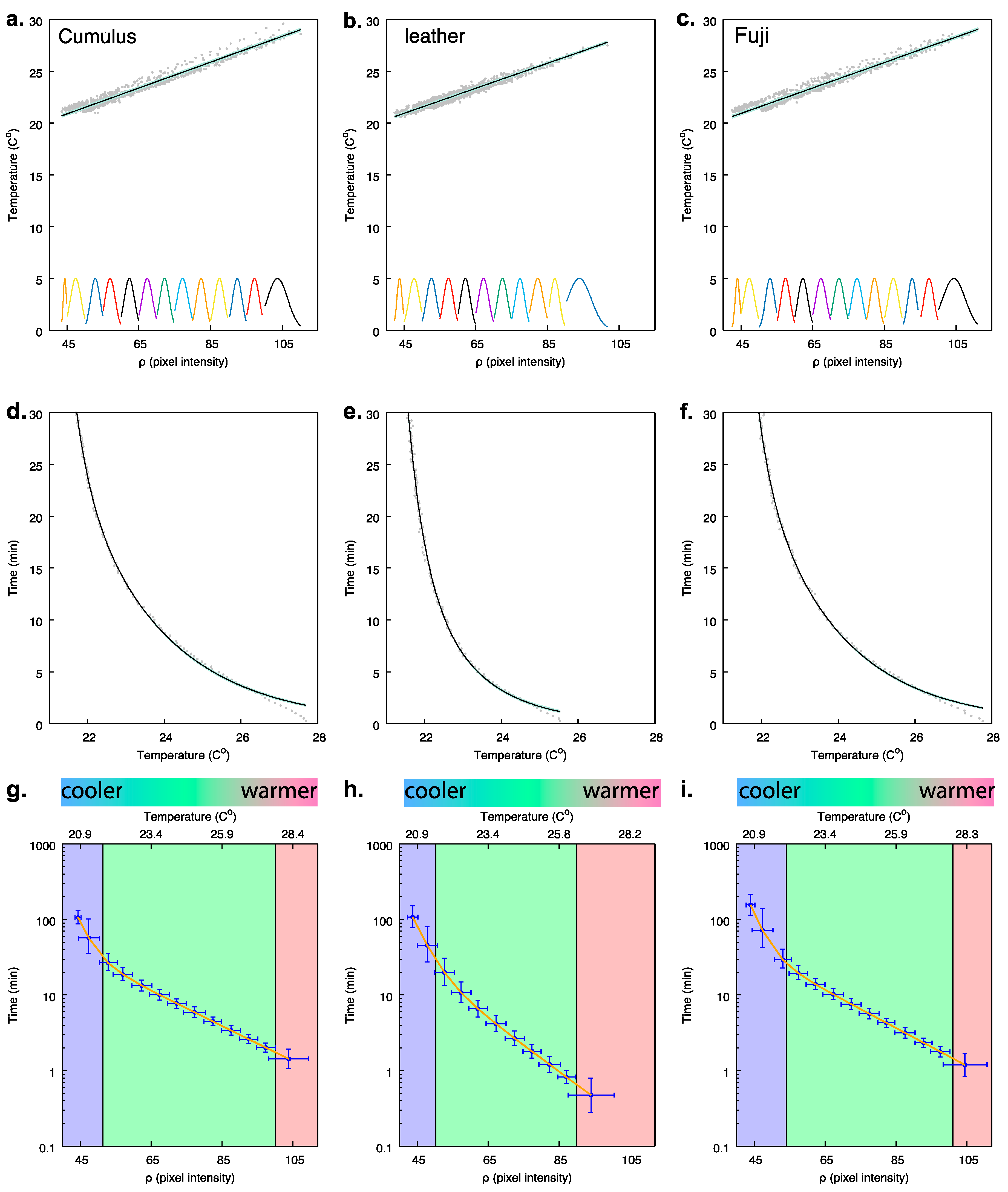
We found a linear relationship between pixel intensity level and temperature for the three types of shoes tested in our experiments (Figure 3a–c). In all three cases, camera response significantly predicted temperature (Table 1).
The four coefficients defining the bi-exponential function used to model the cooling rate of the three tested shoes were found to be significant at an α-level = 0.05 (Table 2). However, time predictions corresponding to the first 2.5 to 3 min of the cooling process should be interpreted with care as the function fit for these points is low (Figure 3d–f).
4. Discussion
In the present study, we empirically established time estimates from the cooling rate of a shoe in typical household conditions based on the readings of a commercial grade thermal imager. Results indicate that our method can produce accurate time estimates when the shoe’s temperature is between 27 to 22 °C, roughly corresponding to 3 to 25 min after the shoe has been removed (green region, panels g–i, Figure 3). However, time intervals do show some variation depending upon the material of the shoe (panels d–f, Figure 3), and so we recommend that, for very precise time estimates, it is important to take shoe style into consideration. Thus, for very precise results, validation using the principles we outline would ideally consider local climate conditions like temperature and humidity, and specific sensors that might be employed by a policing department. Despite this variation, the thermal camera can easily and robustly establish if a shoe was worn for time periods less than 15 min, and up to 25 min if shoe style is calibrated. Outside of these time limits, the uncertainty associated with the time estimation greatly increases, and data should be interpreted with care (blue and red regions, panels g–i, Figure 3).
It is common in forensic practice to estimate time from cooling processes, as, for example, when estimating the time of death from the rectal temperature of a corpse [23]. Even though the cooling of an object can be described algebraically by a practical empirical formulation accounting for the effects of conduction, convection, and radiation which involves a single exponential term, i.e., Newton’s Law of Cooling [29], more complex functions are required to accommodate practical aspects of the cooling process [30]. For example, Marshall [30] experimentally determined post-mortem cooling functions with two exponential terms for predicting time of death. This method reliably predicts time of death at ambient temperature under standardised conditions of cooling from a single temperature reading [23]. Likewise, the experimentally determined cooling functions of the shoes were better modelled by an expression using two exponential terms (panels d–f, Figure 3). This suggests the method we show may have much wider implications for collecting thermal evidence with a time signature, although we encourage that specific validation is done to comply with standards of evidence for presentation in court [5,6].
Longer experimental times past 30 min did not allow a clear distinction of time function due to the exponential nature of cooling when the temperature of the shoe came close to room temperature (panels d–f; blue region, panels g–i; Figure 3). When the temperature of the shoe approaches ambient temperature, the temperature gradient between the two decreases and the cooling rate diminishes. Under these conditions, the thermal imager can no longer accurately assign different pixel intensity levels to the two objects due to its NETD and, consequently, the same pixel intensity level is observed during a longer time lapse. This is reflected in the increased uncertainty of the time estimate (y-axis error bar in panels g–i, Figure 3) at the lower end of the sampled temperatures for the three shoes (blue region, panels g–i, Figure 3). The opposite is observed during the first three minutes after the shoe has been removed from the foot, when it is warmest. During this period, the temperature gradient between the shoe and the ambient is large and rapid cooling occurs (panels d–f; red region, panels g–i). As the data was collected every 15 s for the entire experiment, during the initial phase of the cooling process, large changes in intensity levels lead to an increased spread in ρ values (panels a–c, Figure 3). This resulted in large uncertainty along the x-axis of the cooling function for this period (panels g–i, Figure 3). The value of knowing these error rates for precise thermal imaging in a realistic room scenario is that it allows for robust interpretation of evidence to comply with modern forensic standards [5,6].
Portable commercial thermal cameras, such as the FLIR i50, maintain a linear relationship between the temperature recorded at the sensor level and digital output (ρ) (panels a–c, Figure 3). This is advantageous for quantitative analysis and provides an accurate means of evidence collection in field conditions. Moreover, the linear response of the thermal imager suggests that fewer steps are required for characterising this device for technical and forensic uses compared to other systems for imaging in the UVA and visible regions [2,8]. In these devices, camera characterisation protocols include a dedicated linearisation step before quantitative image analyses can be performed [2,8]. Therefore, the relatively easier characterisation of commercially available ‘off the shelf’ thermal imaging devices may facilitate its popularisation among forensic practitioners and law enforcement agents. Future calibration studies including larger samples of each shoe type and accounting for the potential effects of other environmental factors, such as humidity and variations of the surrounding ambient temperature, should be performed to further validate our method.
Estimating time from temperature measurements of common materials using analytical methods is difficult as the material’s cooling function is determined by the efficiency at which heat is transferred to the ambient environment, i.e., its emissivity [22]—a parameter which is difficult to accurately assess even in laboratory conditions [21]. For example, the leather shoe used in our experiments is more efficient at transmitting heat than the running shoes, as evidenced by the slope of their cooling functions (panels d–f, Figure 3). This result suggests that there are potential differences between the emissivity values of these two materials. Therefore, if the precise emissivity value of an object found in a crime scene is unknown, it is not possible to directly use its temperature to estimate cooling time. However, by using digital images from an empirically calibrated thermal imager, the effect of emissivity is accounted for as part of the calibration process that we demonstrate, thus allowing a first responder to a crime scene to use thermal readings from different materials to obtain reliable time estimates.
Our experiment demonstrates the feasibility of developing a portable device that law enforcers can use to obtain time estimates of the presence, or absence, of a potential suspect in a residential location following a careful calibration protocol. By using a data-driven characterisation, images produced by this method can give litigable evidence to verify claims about the whereabouts of a person of interest in the previous 20 min or after being followed to a location.
The imaging characterisation method proposed here can be easily extended to include other applications, such as to ascertain the presence of suspected illicit marijuana farms in urban environments. Common signs of home grown marijuana are the “glowing” of the habitational unit in thermal images due to the requirements for an indoor greenhouse [31]. Similar to the cooling of the shoe, where pixel intensity decreases over time, the pixel intensity of the house of interest would slowly change until reaching the same level as their surrounding house once the power has been turned off to mislead the authorities. In this context, time estimates from thermal images can be used as evidence to corroborate witnesses’ or suspects’ testimonies or for cross-examination during trial, or could be used in biological and medical studies [32,33]. By implementing scientific principles to calibrate thermal imagers, these devices could be more frequently used for criminal investigation and forensic visualisation, giving law enforcers, prosecutors, and attorneys evidentiary tools that stand up to scrutiny in court.
Supplementary Materials
The following are available online at www.mdpi.com/2313-433X/4/1/21/s1.
Acknowledgments
We thank Mani Shrestha for his help on providing the equipment and training required to collect surface temperature measurement. We gratefully acknowledge the expert feedback of three anonymous reviewers and the editor for comments on previous drafts of the manuscript. A.G.D. was supported by Australian Research Council Discovery Projects grant DP160100161 and DP130100015.
Author Contributions
Adrian G. Dyer, Jair E. Garcia and Justin H. J. Chua conceived and designed the experiments; Justin H. J. Chua performed the experiments; Adrian G. Dyer, Jair E. Garcia and Justin H. J. Chua analyzed the data; Adrian G. Dyer, Jair E. Garcia and Justin H. J. Chua contributed reagents/materials/analysis tools; Adrian G. Dyer, Jair E. Garcia and Justin H. J. Chua wrote the paper.
Conflicts of Interest
The authors declare no conflict of interest.
References
- Robinson, E.M.; Richards, G.B. Chapter 12—Legal issues related to photographs and digital images. In Crime Scene Photography, 2nd ed.; Academic Press: San Diego, CA, USA, 2010; pp. 583–649. [Google Scholar]
- Garcia, J.E.; Wilksch, P.A.; Spring, G.; Philp, P.; Dyer, A. Characterization of digital cameras for reflected ultraviolet photography; implications for qualitative and quantitative image analysis during forensic examination. J. Forensic Sci. 2014, 59, 117–122. [Google Scholar] [CrossRef] [PubMed]
- McKechnie, M.L.; Porter, G.; Langlois, N. The detection of latent residue tattoo ink pigments in skin using invisible radiation photography. Aust. J. Forensic Sci. 2008, 40, 65–72. [Google Scholar] [CrossRef]
- Spring, G. Forensic photography. In The Focal Encyclopedia of Photography, 4th ed.; Peres, M.R., Ed.; Focal Press/Elsevier: Burlington, NJ, USA, 2007; pp. 535–537. [Google Scholar]
- Merlino, M.L.; Springer, V.; Kelly, J.S.; Hammond, D. Meeting the challenges of the daubert trilogy: Refining and redefining the reliability of forensic evidence. Tulsa Law Rev. 2007, 43, 417–446. [Google Scholar]
- Edwards, H.; Gotsonis, C. Strengthening Forensic Science in the United States: A Path Forward; National Academies Press: Washington, DC, USA, 2009. [Google Scholar]
- Dyer, A.G.; Muir, L.L.; Muntz, W.R.A. A calibrated grey scale for forensic ultraviolet photography. J. Forensic Sci. 2004, 49, 1056–1058. [Google Scholar] [CrossRef] [PubMed]
- Garcia, J.E.; Dyer, A.G. UV digital imaging: New perspectives for quantitative data analysis in forensics. In Forensic Science: New Developments, Perspectives and Advanced Technologies; Brewer, J., Ed.; Nova Science Publishers: Hauppauge, NY, USA, 2015; pp. 1–23. [Google Scholar]
- Finney, A. Infrared photography. In The Focal Encyclopedia of Photography: Digital Imaging, Theory and Applications, History, and Science, 4th ed.; Peres, M.R., Ed.; Elsevier/Focal Press: Burlington, NJ, USA, 2007; pp. 556–562. [Google Scholar]
- Oliver, W.R.; Leone, L. Digital UV/IR photography for tattoo evaluation in mummified remains. J. Forensic Sci. 2012, 57, 1134–1136. [Google Scholar] [CrossRef] [PubMed]
- Cosentino, A. Identification of pigments by multispectral imaging; a flowchart method. Heritage Sci. 2014, 2, 8. [Google Scholar] [CrossRef]
- Gashi, B.; Edwards, M.R.; Sermon, P.A.; Courtney, L.; Harrison, D.; Xu, Y. Measurement of 9 mm cartridge case external temperatures and its forensic application. Forensic Sci. Int. 2010, 200, 21–27. [Google Scholar] [CrossRef] [PubMed]
- Petkovšek, M.; Dular, M. Observing the thermodynamic effects in cavitating flow by IR thermography. Exp. Therm. Fluid Sci. 2017, 88, 450–460. [Google Scholar] [CrossRef]
- Castillo, R.V.; Pérez-Lara, M.A.; Rivera-Muñoz, E.; Arjona, J.L.; Rodríguez-García, M.E.; Acosta-Osorio, A.; Galván-Ruiz, M. Thermal imaging as a non-destructive testing implemented in heritage conservation. J. Geogr. Geol. 2012, 4, 102. [Google Scholar] [CrossRef]
- Company, E.K. Applied Infrared Photography; Eastman Kodak Company: Rochester, NY, USA, 1972. [Google Scholar]
- Holst, G.C.; Lomheim, T.S. CMOS/CCD Sensors and Camera Systems; SPIE Press: Bellingham, WA, USA, 2007. [Google Scholar]
- Ray, S. Scientific Photography and Applied Imaging, 1st ed.; Focal Press: Boston, MA, USA, 1999. [Google Scholar]
- Wyszecki, G.; Stiles, W.S. Color Science Concepts and Methods, Quantitative Data and Formulae, 2nd ed.; John Wiley & Sons, Inc.: New York, NY, USA, 1982. [Google Scholar]
- Gaussorgues, G. Infrared Thermography; Chapman & Hall: London, UK, 1994. [Google Scholar]
- Gonzalez, R.C.; Woods, R.E. Digital Image Processing, 3rd ed.; Pearson Prentice Hall: Upper Saddle River, NJ, USA, 2008. [Google Scholar]
- Budzier, H.; Gerlach, G. Thermal Infrared Sensors: Theory, Optimisation and Practice; John Wiley & Sons: Chichester, UK, 2011. [Google Scholar]
- Moran, M.J.; Shapiro, H.N.; Boettner, D.D.; Bailey, M.B. Fundamentals of Engineering Thermodynamics; John Wiley & Sons: Hoboken, NJ, USA, 2010. [Google Scholar]
- Henßge, C.; Madea, B. Estimation of the time since death in the early post-mortem period. Forensic Sci. Int. 2004, 144, 167–175. [Google Scholar] [CrossRef] [PubMed]
- Schneider, C.A.; Rasband, W.S.; Eliceri, K.W. NiH image to imageJ: 25 years of image analysis. Nat. Methods 2012, 9, 671–675. [Google Scholar] [CrossRef] [PubMed]
- Gelman, A.; Hill, J. Data Analysis Using Regression and Multilevelhierarchical Models; Cambridge University Press: New York, NY, USA, 2007; Volume 1. [Google Scholar]
- Keele, L. Bootstrapping. In Semiparametric Regression for the Social Sciences; John Wiley & Sons: Sussex, UK, 2008; pp. 177–193. [Google Scholar]
- Forbes, C.; Evans, M.; Hastings, N.; Peacock, B. Statistical Distributions, 4th ed.; John Wiley & Sons: Hoboken, NJ, USA, 2011. [Google Scholar]
- Delignette-Muller, M.L.; Dutang, C. Fitdistrplus: An R package for fitting distributions. J. Stat. Softw. 2015, 64, 1–34. [Google Scholar] [CrossRef]
- Giancoli, D.C. Physics Principles with Applications, 5th ed.; Prentice Hall: Upper Saddle River, NJ, USA, 1998. [Google Scholar]
- Marshall, T.K. Temperature methods of estimating the time of death. Med. Sci. Law 1965, 5, 224–232. [Google Scholar] [CrossRef] [PubMed]
- Cervantes, J. Marijuana Horticulture: The Indoor/Outdoor Medical Grower’s Bible; Van Patten Publishing: Vancouver, WA, USA, 2006. [Google Scholar]
- Norgate, M.; Boyd-Gerny, S.; Simonov, V.; Rosa, M.G.P.; Heard, T.A.; Dyer, A.G. Ambient temperature influences Australian native stingless bee (Trigona carbonaria) preference for warm nectar. PLoS ONE 2010, 5, e12000. [Google Scholar] [CrossRef] [PubMed]
- Ring, E.F.J.; Ammer, K. Infrared thermal imaging in medicine. Physiol. Meas. 2012, 33, R33–R46. [Google Scholar] [CrossRef] [PubMed]
Figure 1.
Spectral emission from ideal Planckian radiators heated at different temperatures (solid black lines), and spectral bandwidths commonly used for forensic imaging (colour rectangles). Square markers indicate the maximum amplitude (λmax) for each spectrum: daylight (correlated colour temperature of 6500 K), halogen–tungsten filament (4000 K), 75 W house bulb (2800 K), wax candle (1900 K), hot plate for technical purposes heated at about 370 °C (644 K), human body at 37 °C (310 K), and a black body heated at 20 °C (293 K) and 0 °C (273 K). Note how some sources emit radiation across several spectral bands: ultraviolet (UV), visible (VIS), near infrared (NIR), and intermediate and far infrared. Spectral bands cover the sensitivity range of most common imaging devices used for forensic and technical applications in the ultraviolet, visible, and infrared regions of the electromagnetic spectrum [2,10,11,19,21].

Figure 2.
(a) Temperature sampling points on three adult male shoes and (b) representation of shoe cooling in pilot studies. See text and Figure 3 for quantitative analysis. Points A–E represent temperature sampling points with Therm-Micro probes on points A (External Toe); B (External Heel); C (Internal Toe); D (Internal Heel); E (Internal Point). Circular boxes represent sampled point on the surface of shoe, square boxes represent points internally sampled.

Figure 3.
Experimental data and modelling results for a method allowing the prediction of cooling time of three different shoes—Cumulus (first column), leather (middle column), and Fuji shoe (third column)—from pixel values of a thermal imaging device in typical room conditions after wearing three different types of shoes (refer to Materials and Methods section for details). Panels (a–c) show the relationship between camera response, expressed as pixel intensity values (ρ), and shoe temperature reading of the FLIR i50 30 min after shoe removal. Points represent experimental data, the solid black line represents the predicted function, and the shaded area represents the 95% confidence intervals for the function. The curves at the bottom of each panel represent the shape of the probability density distribution (pdf) of the camera responses at 11 different intensity levels modelled assuming a beta distribution (See Supplementary Materials for coefficients defining each distribution); Panels (d–f) show temperature as a function of time for the tested shoe types modelled assuming a bi-exponential function. Points represent the experimental data from the Temperature Sensor Meter, the solid black line represents the nonlinear regression function, and the shaded area represents the 95% confidence intervals. Panels (g–i) represent the cooling function for each shoe type: (g) Cumulus, (h) leather, and (i) Fuji shoe. Error bars on the x-axis represent 95% confidence intervals for camera responses at different pixel intensity values, whilst error bars on the y-axis represent the 95% confidence intervals of the predicted cooling time. In panels (g–h), the green shaded area represents the temperature range for which time can be reliably predicted from camera responses. Blue and red areas represent areas of high uncertainty where data should be interpreted with caution.

Table 1.
Coefficients and associated 95% confidence intervals for the linear function mapping from pixel intensity values into temperature (Equation (1)). Values in parentheses indicate the lower and upper limit of the 95% confidence intervals for each coefficient.
Table 1.
Coefficients and associated 95% confidence intervals for the linear function mapping from pixel intensity values into temperature (Equation (1)). Values in parentheses indicate the lower and upper limit of the 95% confidence intervals for each coefficient.
| Shoe Type | Coefficient | Value (95% CI) | p-Value |
|---|---|---|---|
| Cumulus | β0 | 15.3 (15.1, 15.5) | <0.001 |
| β1 | 0.125 (0.124, 0.126) | <0.001 | |
| Leather | β0 | 15.5 (15.3, 15.7) | <0.001 |
| β1 | 0.121 (0.120, 0.122) | <0.001 | |
| Fuji | β0 | 15.4 (15.2, 15.6) | <0.001 |
| β1 | 0.123 (0.122, 0.124) | <0.001 |
Table 2.
Coefficients and associated 95% confidence intervals for the bi-exponential function used to model the cooling process of the three different shoe models used for the experiments (Equation (2)). Values in parentheses indicate the lower and upper limit of the 95% confidence intervals for each coefficient.
| Shoe Type | Coefficient | Value (95% CI) |
|---|---|---|
| Cumulus | a (min) | 1.04 × 10⁶ (7.10 × 10⁵, 1.49 × 10⁶) |
| b (°C)−1 | −4.29 × 10⁻¹ (−4.45 × 10⁻¹, −4.14 × 10⁻¹) | |
| c (min) | 1.78 × 1025 (5.74 × 10²², 1.96 × 1027) | |
| d (°C)−1 | −2.52 (−2.74, −2.26) | |
| Leather | a (min) | 9.58 × 10⁷ (1.33 × 10⁷, 3.24 × 10⁸) |
| b (°C)−1 | −6.60 × 10⁻¹ (−7.11× 10⁻¹, −5.78 × 10⁻¹) | |
| c (min) | 8.34 × 10²² (4.85 × 10¹⁹, 2.08 × 1025) | |
| d (°C)−1 | −2.52 (−2.26, −1.91) | |
| Fuji | a (min) | 2.71 × 10⁶ (1.85 × 10⁶, 4.02× 10⁶) |
| b (°C)−1 | −4.69 × 10⁻¹ (−4.85 × 10⁻¹, −4.53 × 10⁻¹) | |
| c (min) | 1.84 × 1026 (1.96 × 10²³, 2.15 × 1028) | |
| d (°C)−1 | −2.61 (−2.83, −2.29) |
© 2018 by the authors. Licensee MDPI, Basel, Switzerland. This article is an open access article distributed under the terms and conditions of the Creative Commons Attribution (CC BY) license (http://creativecommons.org/licenses/by/4.0/).
Share and Cite
MDPI and ACS Style
Chua, J.H.J.; Dyer, A.G.; Garcia, J.E. Hot Shoes in the Room: Authentication of Thermal Imaging for Quantitative Forensic Analysis. J. Imaging 2018, 4, 21. https://doi.org/10.3390/jimaging4010021
AMA Style
Chua JHJ, Dyer AG, Garcia JE. Hot Shoes in the Room: Authentication of Thermal Imaging for Quantitative Forensic Analysis. Journal of Imaging. 2018; 4(1):21. https://doi.org/10.3390/jimaging4010021
Chicago/Turabian StyleChua, Justin H. J., Adrian G. Dyer, and Jair E. Garcia. 2018. "Hot Shoes in the Room: Authentication of Thermal Imaging for Quantitative Forensic Analysis" Journal of Imaging 4, no. 1: 21. https://doi.org/10.3390/jimaging4010021
Note that from the first issue of 2016, this journal uses article numbers instead of page numbers. See further details here.