Stable Image Registration for In-Vivo Fetoscopic Panorama Reconstruction †
by
 ,
,
Floris Gaisser
1,*, 
Suzanne H. P. Peeters
2,
Boris A. J. Lenseigne
1,
Pieter P. Jonker
1 and
Dick Oepkes
2 1
BioMechanical Engineering, Delft University of Technology, 2628CD Delft, The Netherlands
2
Department of Obstetrics, Leiden University Medical Center, 2333ZA Leiden, The Netherlands
*
Author to whom correspondence should be addressed.
†
This paper is an extended version of our paper published in: Gaisser, F.; Peeters, S.H.; Lenseigne, B.; Jonker, P.P.; Oepkes, D. Fetoscopic Panorama Reconstruction: Moving from Ex-vivo to In-vivo. In Annual Conference on Medical Image Understanding and Analysis; Springer: Berlin, Germany, 2017; pp. 581–593.
J. Imaging 2018, 4(1), 24; https://doi.org/10.3390/jimaging4010024
Submission received: 31 October 2017
/
Revised: 8 January 2018
/
Accepted: 9 January 2018
/
Published: 19 January 2018
(This article belongs to the Special Issue Selected Papers from “MIUA 2017”)
Abstract
:A Twin-to-Twin Transfusion Syndrome (TTTS) is a condition that occurs in about 10% of pregnancies involving monochorionic twins. This complication can be treated with fetoscopic laser coagulation. The procedure could greatly benefit from panorama reconstruction to gain an overview of the placenta. In previous work we investigated which steps could improve the reconstruction performance for an in-vivo setting. In this work we improved this registration by proposing a stable region detection method as well as extracting matchable features based on a deep-learning approach. Finally, we extracted a measure for the image registration quality and the visibility condition. With experiments we show that the image registration performance is increased and more constant. Using these methods a system can be developed that supports the surgeon during the surgery, by giving feedback and providing a more complete overview of the placenta.
1. Introduction
The Twin-to-Twin Transfusion Syndrome (TTTS) is a condition involving monochorionic twins (twins with a shared placenta) with an imbalance in blood exchange that occurs through vascular anastomoses (connecting blood vessels) on the shared placenta. It occurs in about 10% of such pregnancies and is a condition that can lead to fatal complications for both twins [1]. It can be treated by fetoscopic laser surgery, a technique to separate the fetal circulation through fetoscopic laser coagulation. This surgery increases the survival rate over other techniques but relies on the condition that all vascular anastomoses have been found [2]. For this the surgeon has to scan the placenta for all places where blood vessels of the two twins connect and accurately note them. Then these vessels have to coagulated in a specific order to restore the blood exchange balance and finally separate the blood circulation of both twins. This scanning procedure is complicated due to the very limited field of view of the fetoscope, lack of proper landmarks on the placenta and bad visibility conditions. A panorama reconstruction of the placenta would greatly reduce the chance of complications of the surgery. Panorama reconstruction of internal anatomical structures has found many applications, such as for retina [3], bladder [4] and esophagus [5] reconstruction. However, fetoscopic panorama reconstruction has mostly been done ex-vivo [6,7,8,9].
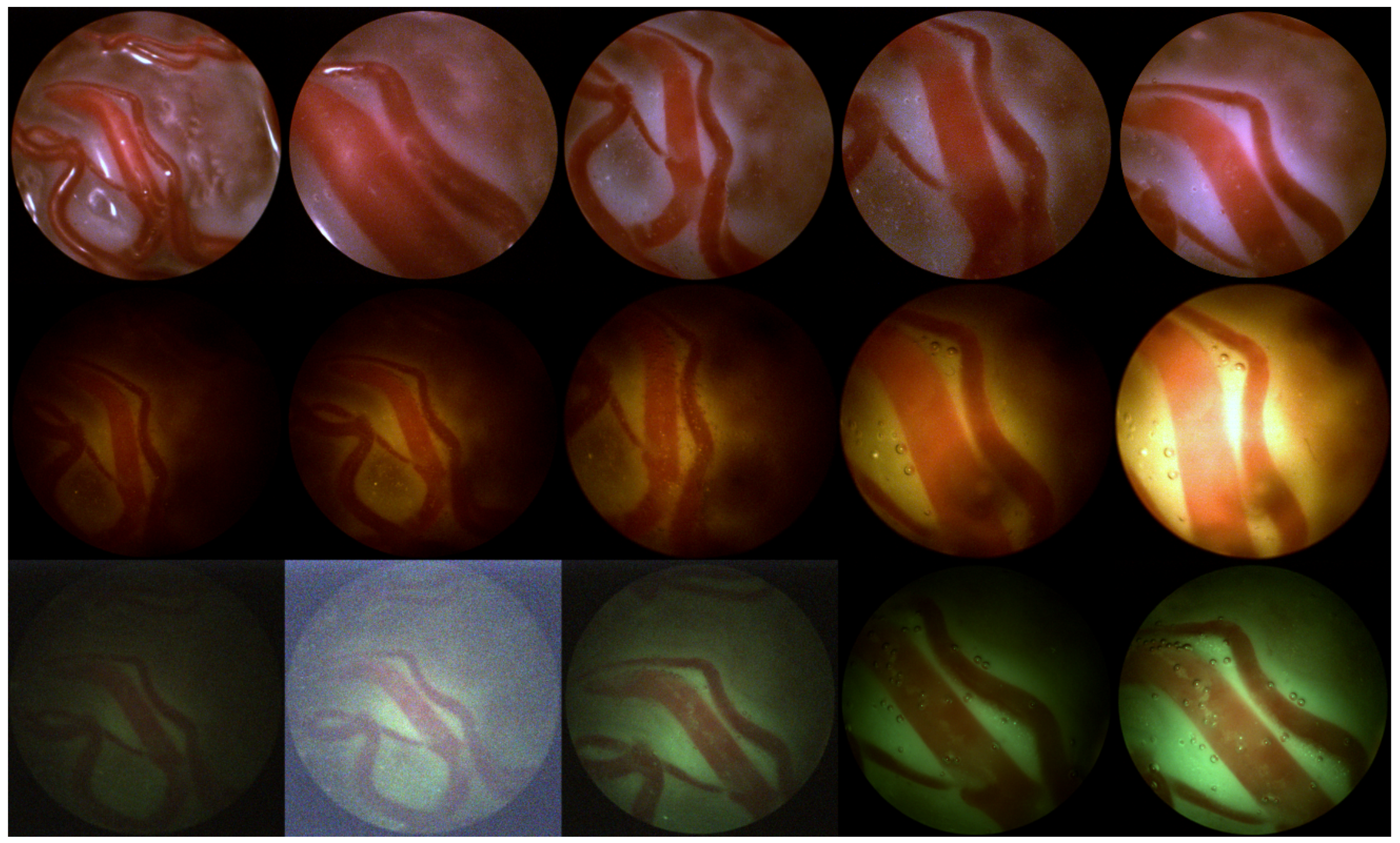
For panorama reconstruction, it is necessary to correctly find all transformations between images constituting the panorama. A transformation between two adjacent images can be estimated by matching key-points in both images, assuming they are correctly matched and the key-points accurately describe the same locations on the placenta. In our previous work we investigated what is necessary to move from ex-vivo to in-vivo fetoscopic panorama reconstruction and we identified specific challenges for an in-vivo setting: The visibility is complicated by the color and turbidity of the amniotic fluid. Also, the bounded motion of the fetoscope continuously changes the distance to the placenta. Lastly, the light intensity of the fetoscope is limited as one cannot blind the fetus. These aspects result in a very small range (Figure A1) in which current key-point methods for image registration can be fruitfully used.
To cope with the problems of an in-vivo setting, we suggest four points of improvement with respect to our previous work: Improve the key-point detection and matching method in order to achieve more robust image registration. Furthermore, detect unavailable or inaccurate image registrations and discard these from the panorama reconstruction. Also, not to create image registration chains, but to register to a part of the panorama. Finally, improve the visibility by obtaining an image quality measure and providing feedback to the surgeon to move the fetoscope in a certain way and the operation assistant to adjust the light source. Of course, also the equipment plays a role in the performance of the panorama reconstruction; i.e., a larger viewing angle improves the field of view and a high dynamic range or low light camera will obtain a larger range of feasible visibility conditions.
In this work in Section 2 we revisit the problems of in-vivo panorama reconstruction and we formulate requirements for proper reconstruction. Then in Section 3 we introduce recent developments in deep-learning and how this can be used to tackle the problems. In Section 4 we evaluate the proposed approach and in Section 5 we discuss the outcome and come to conclusions.
2. Challenges of In-Vivo Setting
In previous work we described key aspects in which an in-vivo setting differs from an ex-vivo setting and we concluded that in contrast with an ex-vivo setting, state-of-the-art key-point methods have a very limited performance in an in-vivo setting. Therefore other approaches e.g., based on deep learning must be found. In this section we recap the differences in setting and how they influence the image registration between two adjacent fetoscopic images, and we conclude with presenting a set of requirements for a proper image registration in in-vivo settings. The next section then describes the methods we propose to adhere to these requirements.
2.1. Differences in Setting
The visibility in fetoscopic images is a key problem that complicates the image registration between two or more images in an in-vivo setting. The first aspect of good visibility is the amount of light as well as an even distribution. In an ex-vivo setting, the amount of light can be completely controlled and positioned. Therefore, an optimal position and an even distribution of light can be obtained. However, in an in-vivo setting this is not the case:
- The amount of light is limited by the light source and cannot be chosen too bright as it might blind the fetus to the point of annoyance such that the fetus becomes restless.
- The amniotic fluid is far from clear as the fetus micurates in it. Moreover, as commonly the case in TTTS, the fetus might release bowel movements due to distress, giving the amniotic fluid a green turbid color. This color and turbidity of the amniotic fluid absorbs light, reducing the distance the light can reach.
- The source of light is the fetoscope itself. This results in an uneven distribution of light, which reduces the amount of illumination towards the edge of the view. Furthermore, saturation of the imaging sensor in the center of the image inhibits proper observation of the structure of the placenta.
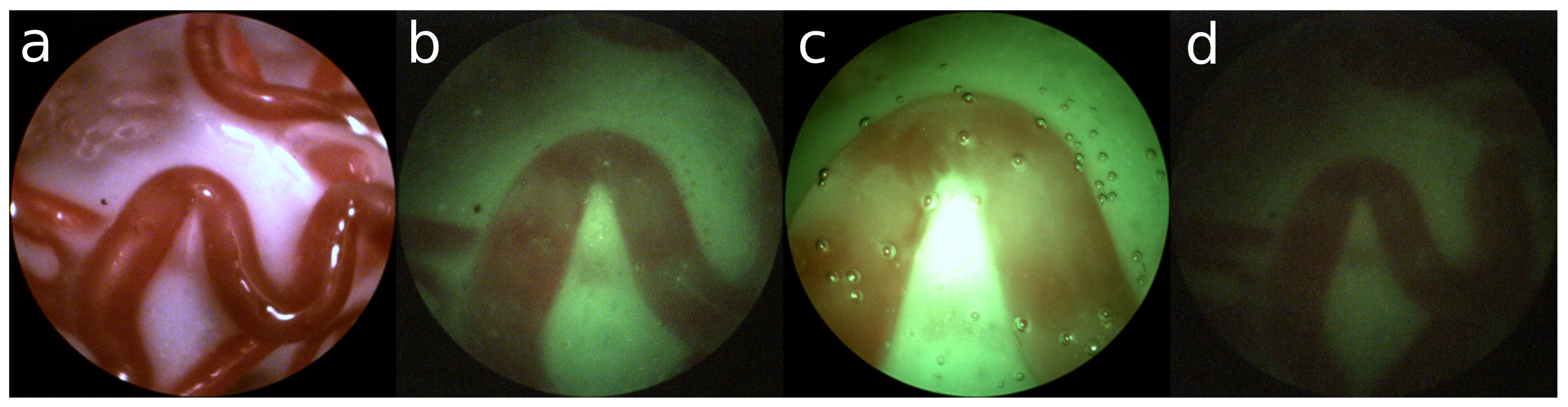
Examples are shown in Figure 1. Especially for the green turbid liquid it is difficult for the camera to acquire a proper image, resulting in a large amount of sensor noise.
The second aspect of good visibility is the distance to the placenta. With enough distance to the placenta it is possible to observe many different structures on the placenta. In an ex-vivo setting the placenta is generally placed on a flat surface and the fetoscope can be positioned at any distance to the placenta. Furthermore, the fetoscope can be moved laterally with equal distance to the placenta. However, this is not the case in an in-vivo setting:
- The distance to the placenta is limited due to the reduced amount of light.
- The fetoscope is limited in motion at the point of entry. It can only rotate around the point of entry and move forward and backward.
- A lateral movement of the field of view can only be obtained by rotation. Therefore, the lateral change of view also changes the distance to the placenta. This results not only in a change of visible structure, but also a change in illumination.
- The scanning procedure in the in-vivo setting is to follow veins from the umbillical cord and back. Which creates large loops, whereas the ex-vivo setting uses a spiraling motion, which has many small loops.
Figure 2a shows an example of an ex-vivo setting with a satisfactory amount of structure. In contrast, Figure 2b shows a nominal example of an in-vivo setting with green turbid liquid. From this point of view, the fetoscope can be moved laterally resulting in a closer view (Figure 2c) or more distant view (Figure 2d). One can observe that suboptimal viewing conditions are unavoidable in an in-vivo setting.
2.2. Influence on Image Registration
For panorama reconstruction, it is necessary to correctly find all transformations between adjacent images constituting the panorama. A transformation between two adjacent images can be estimated with a minimum of 4 matches, assuming they are correctly matched and accurately describe the same locations on the placenta. The key-point matching process assumes that two well matching key-points describe the same physical point. To find matching key-points in two images, the area around a key-point is described with a histogram of gradients. Around corners this generally provides an unique enough description of the key-point such that it can be matched with a similar key-point in an adjacent image. Such a corner is dominated by equally strong gradients in two dimensions. In contrast, along edges, such as along a vein, there is a strong gradient perpendicular to the edge and practically no gradient along the edge. Consequently, key-points selected on an edge are very alike as they have a very similar structure around the point. Moreover, taking sensor noise into account, the histogram of gradients has an additional random component that is often larger than the fine difference between two edges in adjacent images. With a growing variation in the exact location and an increasing number of incorrect matches, the required number of correct matches increases as well. The LMeDS transform estimation method is robust to inaccurate locations, but requires at least correct matches to obtain a transformation [10]. Whereas, the RANSAC method is sensitive to inaccurate locations, though robust to incorrect matches [11]. Unfortunately there is no method that is robust to both inaccurate locations and incorrect matches.
In an in-vivo setting the limited distance to the placenta reduces the observable structure and the limited amount of light creates sensor noise. Hence, unstable key-points are detected that are described by similar features and matching key-points result in many seemingly good, but incorrect matches, describing different points on the placenta, usually along veins. Concluding, in three key aspects traditional key-point matching methods fail in an in-vivo setting; detecting stable key-points, reliable matching of key-points, and obtaining enough matches for a proper estimation of the transform.
2.3. Image Registration Requirements
To research other approaches, such as based on deep learning, it is important to specify the requirements for an image registration process that consistently performs its task in an in-vivo setting:
- Key-points in one image should be reproducible in another image and both should accurately describe the same physical location on the placenta
- The features describing a key-point in one image should be so unique that the matching key-point in another image has almost the same unique features
- Key-points in one image for which no matching key-point is found in the other image should have such unique features that it is not incorrectly matched to key-points in that other image at different locations
- The image registration process should be able to detect whether an obtained transformation is incorrect in order to exclude it from the panorama reconstruction.
The section below describes the method we propose to adhere to these requirements.
3. Method
In recent years, deep-learning neural networks have been applied in many different fields, tackling various complex problems [12]. This approach is successful because it has the ability to learn any complex task without having knowledge on how to solve the task, as long as the desired output is known and enough training data is available. A deep learned network consists of a pipeline of trainable layers, which makes it possible to train the network to handle compound structures.
Convolutional layers are very suitable to extract relevant data from structured data such as images. It is comparable to convolutional filtering the image, but then with filter coefficients that are trained instead of coefficients determined by a user. A convolutional layer has a set of filters that is moved over the input image extracting relevant structures everywhere in the image. This can be applied in many different applications, notably in image classification [13].
In this work we propose a deep convolution neural network to tackle the challenges stated in the previous section. With it we will:
- Detect stable regions on the veins of the placenta
- Extract matchable features from these regions
- Learn a visibility and matchability measure of an image
These steps are detailed in the next sub-sections.
3.1. Stable Region Detector
Soon after the introduction of deep learning it was also applied to the detection of key-points [14,15,16]. These methods are similar to handcrafted methods such as SIFT and ORB, but have the advantage that the networks can be trained to select key-points that are more apt for matching and image registration. Although these networks are often trained with key-points detected by a handcrafted method, this is not very suitable for our case and another way of obtaining a key-point training set needs to be found.
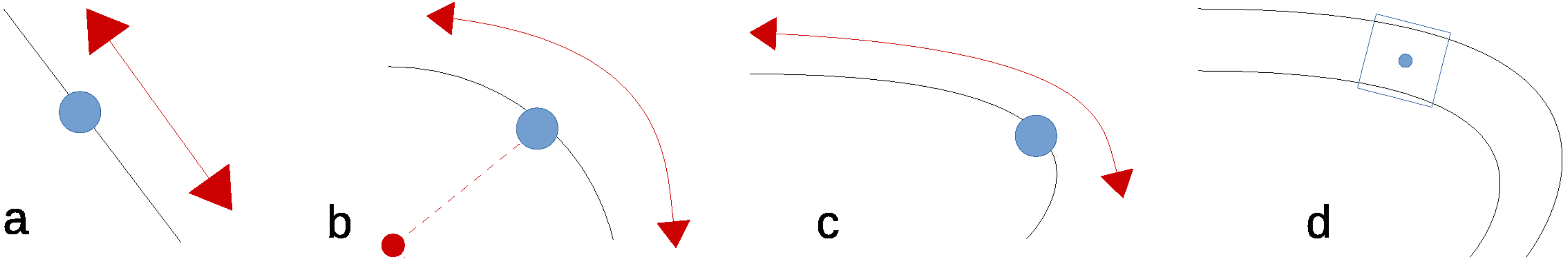
Image registration requires the detection of stable key-points, but it is yet unclear what defines a stable key-point not being a corner. A straight edge (Figure 3a) constraints the key-point in one direction. This is also the case for a circular edge, when rotation is also taken into account, as shown in Figure 3b. However, key-points with the same curvature can be matched. On curved edges, having an additional change in scale, the matching becomes more unique, but not unique enough to do the job (Figure 3c). Therefore, any edge alone, albeit curved, cannot be considered a source of stable key-points. We need additional information to make the key-point unique.
Consequently, we propose to define stable key-points being center points on the medial axis of the veins. As both sides of the vein are curves of different curvature they provide independent constraint dimensions making the point more unique. When also the width of the vein is taken into account this constraints the detection also in the dimension of scale, as shown in Figure 3d. This makes our proposed method less a key-point detector but rather a region detector; we use three instead of two independent dimensions.
Since our approach resembles region/object detection rather than key-point detection, we investigated also Region Convolutional Neural Networks such as RCNN [17], Fast-RCNN [18], Faster-RCNN [19] and Single Shot Detector (SSD) [20], which have been developed to detect and classify objects in images. Earlier methods such as RCNN and Fast-RCNN used external region proposal methods, but Faster-CNN and SSD use the same convolutional network for classification as for region proposals, where SSD detects objects at multiple scales. Therefore, this last method was chosen as basis for our stable region detection method.
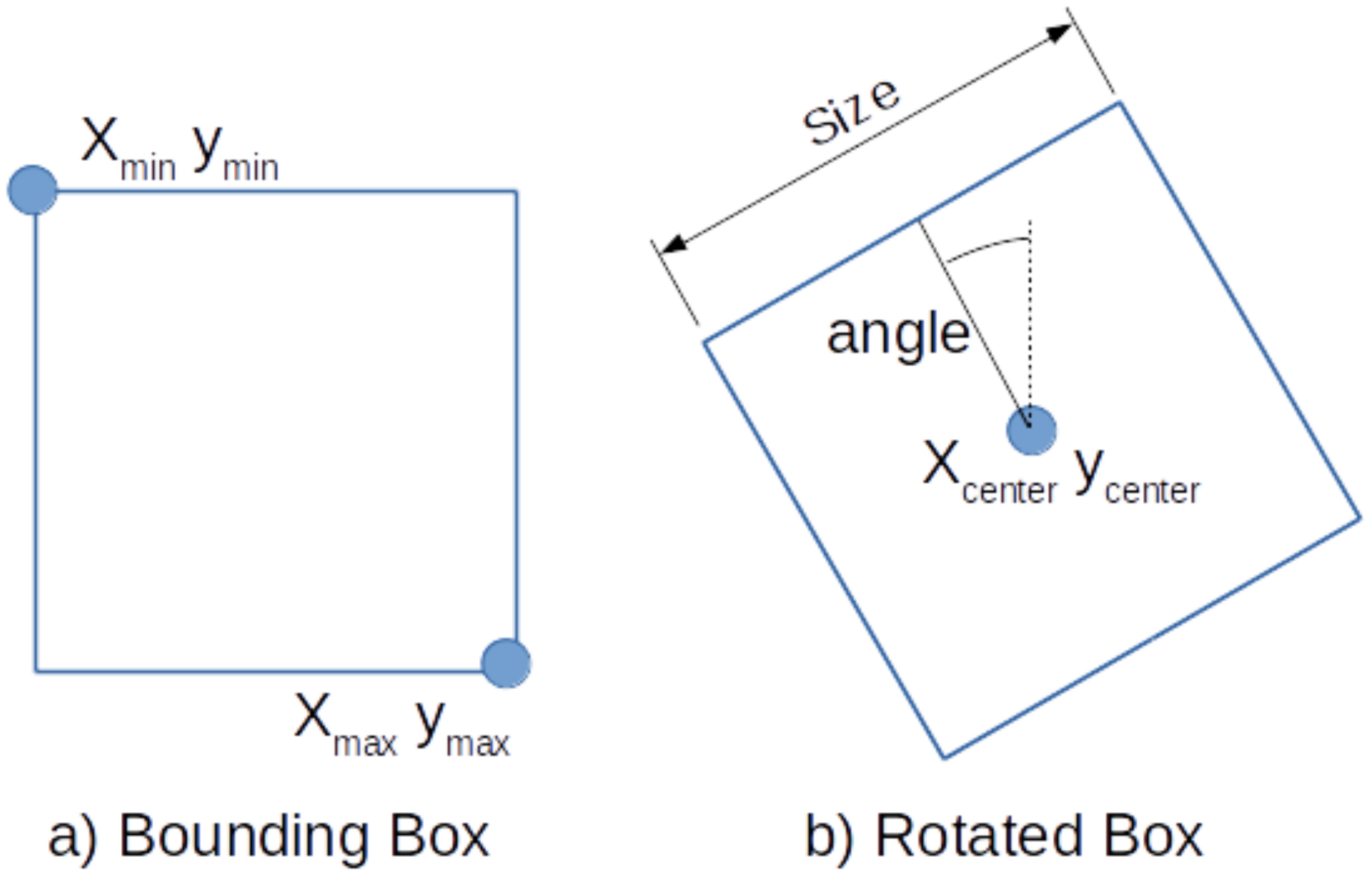
The SSD method detects regions by defining bounding boxes with their min and max corners as shown in Figure 4a. These are learned by training the neural network to output the location of the two corners for each feature cell according to their default boxes. An additional classification layer learns the detection probability of each class in every default box. If the classification layer outputs a positive classification, the matching output of the detection layer is used for localization of the classified object. We refer to the Faster-RCNN [19] and SSD [20] papers for more details on the specifics on how to train these detectors.
In order to detect stable regions on the placenta, we propose to detect square areas on the veins. However, the bounding boxes as defined by SSD are not suitable to describe the orientation of the vein. Therefore, we extent SSD and redefine the default boxes by the center, the size, and the angle of the box, as shown in Figure 4b.
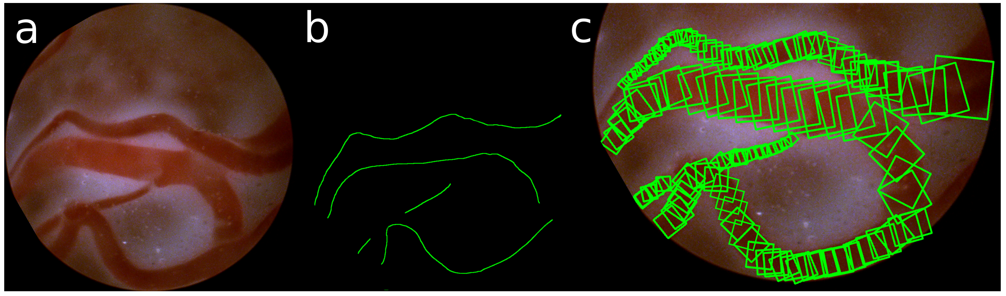
The ground truth of these detections is obtained by manually annotating the center and the radius of the veins in the images. Taking the gradient of these annotations, also the direction of the vein is defined. An example of such annotation of the veins is shown in Figure 5.
It is interesting to note that the definition of our points of stable-regions are similar to that of key-points. Similar to a key-point we also extract features around a location of a rotated box. But whereas key-points are solely defined by a point, a scale and an orientation of the key-point, we restrict the possible locations to be at the center of a vein. This makes them stable and within some margin also reproducible.
3.2. Stable Matching
The second challenge in the image registration process is to extract features that are descriptive enough for the proper matching of key-points. In [15], this was achieved by training with positive and negative samples, using Euclidean distance to measure similarity in a Siamese CNN. This is similar to [7] where patches were selected in a grid to extract features that were trained in a Siamese CNN with contrastive loss.
In this paper we extended the SSD architecture similarly to [7]. An additional convolution layer extracts a feature for the detection of Contrastive Loss. Furthermore, every detection is fine-tuned with its matching performance such that detections that are difficult to match are assigned a lower probability to be detected. In this way we remain with matchable features.
3.3. Qualitative Measures
Our last challenge is to obtain a measure of success for the image registration. This can be used to guide the surgeon or/and his assistant. For this, a qualitative measure is trained by using the matching performance which was used to train matchable features. Since the images registration is highly influenced by the visibility, we define two more outputs to describe this visibility. One describes the amount of illumination and the other describes the distance to the placenta. The visibility is defined as optimal in nominal illumination and distance conditions.
These outputs provide an indication about the performance of the image registration. In case of bad registration the images can be discarded in the process. However, to obtain a sequence of images that is continuous, the surgical team should be included in the process, i.e., the surgeon should be made aware that the panorama reconstruction process has lost position. Furthermore, an assistant controlling the light intensity should be made aware of the illumination condition to actively adjust this.
3.4. Network Architecture
The above described contributions are implemented based on the VGG-16 network with SSD as a starting point. In order to detect stable regions, we first associate detection scales with the annotated veins of various sizes and select only the first four levels as a scale space pyramid to detect rotated boxes. Each detection scale by default consists of three layers; first the classification layer for determining if there is a positive detection. Second, the location layer describing the location of the detection and third the prior boxes, describing the template detections. Every scale also passes on the features to the next scale.
Next, for stable matching we change two aspects; First, the SSD network was made into two parallel pipelines as shown in Figure 6a. These two networks share their weights as a Siamese Neural Network. Second, each detection scale is extended with an additional convolutional layer to extract a feature describing every detection as shown in Figure 6b. These, combined with the region detections can be used to find the matches for image registration.
Finally, to extract a measure for visibility and image registration performance, the bottom most detection scale is extended with a convolution layer, a max pooling layer and a convolution layer for classification.
4. Experiments
We performed various experiments to show how our method can handle the image registration challenges encountered in an in-vivo setting. For this we used data from our previous work with various visibility conditions. For training, we selected two sets of data, an ex-vivo setting and an in-vivo setting, including both nominal conditions for yellow and green amniotic fluid. For each setting a minimum of 25 and a maximum of 42 images were obtained for the same trajectory on the placenta. The number of images vary because of the differences in visibility. In total 745 images were used for various settings.
The training data was augmented by rotating the image in steps of 45 degrees and flipping it, such that 16 variations are obtained. For testing, all variations in visibility are used. Therefore, in nominal conditions of the total set is used for testing and the rest is used for training. For all other visibility conditions all data is used for evaluation.
4.1. Experiment 1—Stable Region Detector
The stable region detector as proposed in Section 3.1 should detect the center of the vein. Therefore, we manually annotated the center and the radius of the veins and extracted the direction of the veins. According to the chosen scales and number of cells in the convolutional layers, the closest annotated point is selected as the ground truth and used to train the stable region detection network.
We evaluated the detection performance of these regions as well as their reproducibility for both the bounding boxes (BBox) and rotated boxes (RBox). We applied a confidence threshold of and obtained on average , with a minimum of 11, regions per image in the in-vivo setting. With this high threshold the performance is also very high with correctly detected regions. Lowering the threshold provides more regions albeit that the precision goes down very quickly. Below only incorrect regions are detected. Therefore, we used this threshold of in the rest of our experiments. The results of the BBox detections with more thresholds are shown in Table 1.
To determine the reproducibility of the detected regions, the transform between two successive images have been manually established. The ratio of the detections in two adjacent images that describe the same area are obtained by transforming the detections from one image to the other. The reproducible number of detections is on average of the detected regions for the ex-vivo, and for the in-vivo settings and . For all visibility conditions an overview is presented in Table A1. It also provides a comparison with the results of the key-point methods from our previous work.
4.2. Experiment 2—Stable Region Matching
To obtain matchable features we trained the neural network with Contrastive Loss on the matches. To evaluate the matching performance of our approach, the true matches from the previous experiment are used and compared to the number of matched regions. For the nominal ex-vivo setting and for the nominal in-vivo settings and were correctly matched. For these settings all images had enough stable matches to obtain image registration. Furthermore, the mean pixel error was less than 2 pixels using LMeDS as the transform estimation method. Table A2 shows the matching performance for the other more challenging settings than nominal. For some visibility conditions an insufficient ratio of correct matches were found to use LMeDS, thus RANSAC was used instead.
4.3. Experiment 3—Qualitative Measure
To obtain a qualitative measure for the matching process as a whole for two adjacent images, the performance of the previous experiment is defined as bad if no transformation could be found either by having not enough detected regions or having not enough correctly matched pairs. A good performance is defined by more than correct matches and a minimum of 6 correct matches. Which is based upon the requirement of LMeDs of having at least correct matches and having more than 4 matches to handle location inaccuracy. By training an output with these labeled outcomes a measure of matchability could be obtained.
To obtain a qualitative measure of the visibility, a dataset was created containing also the dark, light, close and far visibility conditions. For the illumination and distance variation the nominal situation was defined as 0 and the two extremes of the variation as either or 1 and trained with Euclidean loss. Table 2 shows the results for the qualitative measures as a ratio of giving a correct indication and an overall correct indication of successful image registration, where these measures are combined for the nominal setting.
5. Discussion
In this paper we proposed an extension of an SSD network to detect regions in fetoscopic images with stable matchable features. With the same network architecture we also obtain a measure of matchability for the purpose of obtaining a sufficient set of matchable regions of consistent quality for proper image registration.
In Experiment 1 we showed that it is possible to detect stable regions on the placenta based on the medial axis of veins, under visibility conditions encountered in an in-vivo setting. Compared to key-point methods our approach only detects a limited number of regions, albeit that the number of reproducible regions is much higher and more consistent over all adjacent images in a trajectory.
The method to learn matchable feature was evaluated in Experiment 2. It showed that in better visibility conditions, a high percentage of correct matches could be obtained and that the number of correct matches is especially in darker settings reduced. Therefore, in the more complicated settings sometimes not enough matches could be found to obtain a transformation. However, in the nominal settings for of the images sufficient matches could be found to obtain a transform.
These results show again that the visibility greatly complicates the in-vivo setting. First, for both the yellow and green-turbid liquid, the darker conditions have not enough contrast to provide the required detail to detect enough regions and extract matchable features. Next, the distance to the placenta also reduces the amount of regions that can be detected, resulting in not enough matches to either use LMeDS or obtain a transform estimation. Last, for the green-turbid settings, many images contain a large amount of sensor noise. These images provide a large number of key-points, however with our region detection method, almost no stable region could be detected.
The transform estimation precision is not as accurate as we expected. It seems that also our region detection method does not describe the same physical location uniquely enough. A more accurate transform estimation should be obtainable with dense optimization. This is anyway required for panorama reconstruction of large sequences without loops.
As stated it will still be very difficult to estimate a correct transform for all different visibility conditions. Therefore, in these cases it is important to be able to detect that the visibility condition is not suited for image registration. Experiment 3 evaluates the three qualitative measures defined and their combination for image registration. In most cases it is possible to detect whether the image is suitable for image registration. Furthermore, as the visibility condition is of great influence on the construction of the panorama image, this visibility should be communicated to the surgical team such that they can adjust the visibility at certain points on the panorama.
6. Conclusions
The aim of this work was to improve the panorama reconstruction process for in-vivo fetoscopic imaging. Our starting point was given by the four recommended points of improvement as described in our previous work. First, we improved the key-point detection and matching method, by extending the SSD method to detect stable regions and extract matchable features. Next, the panorama reconstruction process was improved, by detecting the complicating visibility conditions for the image registration and discarding improperly matched image pairs. Furthermore, a measure of the visibility condition was extracted such that it can be fed back to the surgical team. In this way, fetoscopic images of higher matchability might be obtained by a retry of the surgical team. These three points of improvement make a crucial step in the direction of in-vivo panorama reconstruction. Note that, the point of improving the equipment itself was not discussed in this work. A major improvement will come from an increased field of view while keeping the diameter of the fetoscope as small as possible.
Author Contributions
Floris Gaisser conceived the presented concept and developed the neural network. Floris Gaisser and Boris Lenseigne performed the experiments. Suzanne Peeters and Dick Oepkes provided and evaluated the experimental setup. Pieter Jonker and Dick Oepkes supervised the findings of the work. Floris Gaisser and Pieter Jonker wrote and all reviewed the manuscript.
Conflicts of Interest
The authors declare no conflict of interest.
Abbreviations
The following abbreviations are used in this manuscript:
| TTTS | Twin-To-Twin Transfusion Syndrome |
| LMeDS | Least Median of Squares |
| RANSAC | Random Sample Consensus |
| RCNN | Region-based Convolutional Neural Network |
| SSD | Single Shot (multibox) Detector |
| BBox | Bounding Box |
| RBox | Rotated Box |
| ex-vivo | Setting outside of and without mimicking the human body |
| in-vivo | Setting inside of or (realistically) mimicking the human body |
| setting | Environmental condition of the (experimental) setup |
| visibility condition | Changable situation influencing the visibility of the fetoscope |
| key-point | Interesting point as detected by methods like SIFT, SURF etc. |
Appendix A. Visibility Conditions
Figure A1.
Variations in viewing conditions. Top row left to right: ex-vivo-far, ex-vivo-close, ex-vivo with water-far, ex-vivo with water-nominal, ex-vivo with water-close; Middle row: yellow liquid, bottom row: green turbid liquid; left to right: far-dark, far-nominal, nominal for both, close-nominal, close-bright.

Appendix B. Detailed Results
Please note that the results of the Key-point methods have been copied from Experiments 1 and 2 from previous work.

Table A1.
Experiment 1: Key-points/regions detected.
| Setting | Condition | Detected | Reproducible | |||||||||
|---|---|---|---|---|---|---|---|---|---|---|---|---|
| SIFT | SURF | ORB | BBox | RBox | SIFT | SURF | ORB | BBox | RBox | |||
| ex-vivo | nominal | 269 | 643 | 470 | 81.8% | |||||||
| dark | close | 14 | 31 | 21 | ||||||||
| dark | nominal | 7 | 26 | 5 | ||||||||
| dark | far | 22 | 50 | 15 | ||||||||
| nominal | close | 42 | 132 | 57 | ||||||||
| Yellow | nominal | nominal | 24 | 110 | 21 | 76.5% | ||||||
| nominal | far | 74 | 174 | 73 | ||||||||
| light | close | 97 | 350 | 108 | ||||||||
| light | nominal | 110 | 525 | 129 | ||||||||
| light | far | 38 | 183 | 32 | ||||||||
| dark | close | 24 | 11 | 25 | ||||||||
| dark | nominal | 11 | 13 | 10 | ||||||||
| dark | far | 210 | 192 | 54 | ||||||||
| nominal | close | 94 | 147 | 137 | ||||||||
| Green | nominal | nominal | 239 | 401 | 98 | 73.6% | ||||||
| nominal | far | 1000 | 1000 | 776 | ||||||||
| light | close | 246 | 434 | 320 | ||||||||
| light | nominal | 1000 | 1000 | 578 | ||||||||
| light | far | 1000 | 1000 | 844 | ||||||||
Table A2.
Experiment 2: Matches found and pixel error with LMeDS; * with RANSAC.
| Setting | Condition | Correctly Matched | Sufficient Matches | Pixel Error | ||||
|---|---|---|---|---|---|---|---|---|
| BBox | RBox | BBox | RBox | BBox | RBox | |||
| ex-vivo | nominal | px | 1.9 ± 0.7 px | |||||
| dark | close | |||||||
| dark | nominal | |||||||
| dark | far | |||||||
| nominal | close | px * | 3.1 ± 1.3 px * | |||||
| Yellow | nominal | nominal | px | 1.9 ± 0.8 px | ||||
| nominal | far | px | 1.9 ± 0.6 px | |||||
| light | close | 3.4 ± 1.3 px * | 3.2 ± 1.3 px * | |||||
| light | nominal | px | 1.9 ± 0.7 px | |||||
| light | far | px | 1.9 ± 0.7 px | |||||
| dark | close | |||||||
| dark | nominal | |||||||
| dark | far | |||||||
| nominal | close | 3.2 ± 1.2 px * | ||||||
| Green | nominal | nominal | px | 2.1 ± 0.8 px | ||||
| nominal | far | |||||||
| light | close | |||||||
| light | nominal | |||||||
| light | far | |||||||
References
- Lewi, L.; Deprest, J.; Hecher, K. The vascular anastomoses in monochorionic twin pregnancies and their clinical consequences. Am. J. Obstet. Gynecol. 2013, 208, 19–30. [Google Scholar] [CrossRef] [PubMed]
- Peeters, S. Training and Teaching Fetoscopic Laser Therapy: Assessment of a High Fidelity Simulator Based Curriculum. Ph.D. Thesis, Leiden University Medical Center, Leiden, The Netherlands, 2015. [Google Scholar]
- Seshamani, S.; Lau, W.; Hager, G. Real-time endoscopic mosaicking. In Medical Image Computing and Computer-Assisted Intervention–MICCAI 2006; Springer: Berlin, Germany, 2006; pp. 355–363. [Google Scholar]
- Soper, T.D.; Porter, M.P.; Seibel, E.J. Surface mosaics of the bladder reconstructed from endoscopic video for automated surveillance. IEEE Trans. Biomed. Eng. 2012, 59, 1670–1680. [Google Scholar] [CrossRef] [PubMed]
- Carroll, R.E.; Seitz, S.M. Rectified surface mosaics. Int. J. Comput. Vis. 2009, 85, 307–315. [Google Scholar] [CrossRef]
- Tella-Amo, M.; Daga, P.; Chadebecq, F.; Thompson, S.; Shakir, D.I.; Dwyer, G.; Wimalasundera, R.; Deprest, J.; Stoyanov, D.; Vercauteren, T.; et al. A Combined EM and Visual Tracking Probabilistic Model for Robust Mosaicking: Application to Fetoscopy. In Proceedings of the IEEE Conference on Computer Vision and Pattern Recognition Workshops, Seattle, WA, USA, 27–30 June 2016; pp. 84–92. [Google Scholar]
- Gaisser, F.; Jonker, P.P.; Chiba, T. Image Registration for Placenta Reconstruction. In Proceedings of the IEEE Conference on Computer Vision and Pattern Recognition Workshops, Seattle, WA, USA, 27–30 June 2016; pp. 33–40. [Google Scholar]
- Reeff, M.; Gerhard, F.; Cattin, P.C.; Székely, G. Mosaicing of endoscopic placenta images. In Informatik für Menschen; Hartung-Gorre Verlag: Konstanz, Germany, 2006. [Google Scholar]
- Liao, H.; Tsuzuki, M.; Kobayashi, E.; Dohi, T.; Chiba, T.; Mochizuki, T.; Sakuma, I. Fast image mapping of endoscopic image mosaics with three-dimensional ultrasound image for intrauterine treatment of twin-to-twin transfusion syndrome. In Medical Imaging and Augmented Reality; Springer: Berlin, Germany, 2008; pp. 329–338. [Google Scholar]
- Rousseeuw, P.J. Least Median of Squares Regression. J. Am. Stat. Assoc. 1984, 79, 871–880. [Google Scholar] [CrossRef]
- Fischler, M.A.; Bolles, R.C. Random sample consensus: A paradigm for model fitting with applications to image analysis and automated cartography. Commun. ACM 1981, 24, 381–395. [Google Scholar] [CrossRef]
- LeCun, Y.; Bengio, Y.; Hinton, G. Deep learning. Nature 2015, 521, 436–444. [Google Scholar] [CrossRef] [PubMed]
- Simonyan, K.; Zisserman, A. Very Deep Convolutional Networks for Large-Scale Image Recognition. arXiv, 2014; arXiv:1409.1556. Available online: https://arxiv.org/abs/1409.1556 (accessed on 12 January 2018).
- Verdie, Y.; Yi, K.; Fua, P.; Lepetit, V. TILDE: A temporally invariant learned detector. In Proceedings of the IEEE Conference on Computer Vision and Pattern Recognition, Boston, MA, USA, 7–12 June 2015; pp. 5279–5288. [Google Scholar]
- Simo-Serra, E.; Trulls, E.; Ferraz, L.; Kokkinos, I.; Fua, P.; Moreno-Noguer, F. Discriminative learning of deep convolutional feature point descriptors. In Proceedings of the IEEE International Conference on Computer Vision, Santiago, Chile, 7–13 December 2015; pp. 118–126. [Google Scholar]
- Yi, K.M.; Trulls, E.; Lepetit, V.; Fua, P. Lift: Learned invariant feature transform. In European Conference on Computer Vision; Springer: Berlin, Germany, 2016; pp. 467–483. [Google Scholar]
- Girshick, R.; Donahue, J.; Darrell, T.; Malik, J. Rich feature hierarchies for accurate object detection and semantic segmentation. In Proceedings of the IEEE Conference on Computer Vision and Pattern Recognition, Washington, DC, USA, 23–28 June 2014; pp. 580–587. [Google Scholar]
- Girshick, R. Fast R-CNN. In Proceedings of the IEEE International Conference on Computer Vision, Santiago, Chile, 7–13 December 2015; pp. 1440–1448. [Google Scholar]
- Ren, S.; He, K.; Girshick, R.; Sun, J. Faster R-CNN: Towards real-time object detection with region proposal networks. In Advances in Neural Information Processing Systems; IEEE: Piscataway Township, NJ, USA, 2015; pp. 91–99. [Google Scholar]
- Liu, W.; Anguelov, D.; Erhan, D.; Szegedy, C.; Reed, S.; Fu, C.Y.; Berg, A.C. SSD: Single shot multibox detector. In European Conference on Computer Vision; Springer: Berlin, Germany, 2016; pp. 21–37. [Google Scholar]
Figure 1.
(a) Ex-vivo view; (b) uneven distribution of light; (c) too much light saturating the sensor; (d) not enough light creating sensor noise.
Figure 1.
(a) Ex-vivo view; (b) uneven distribution of light; (c) too much light saturating the sensor; (d) not enough light creating sensor noise.
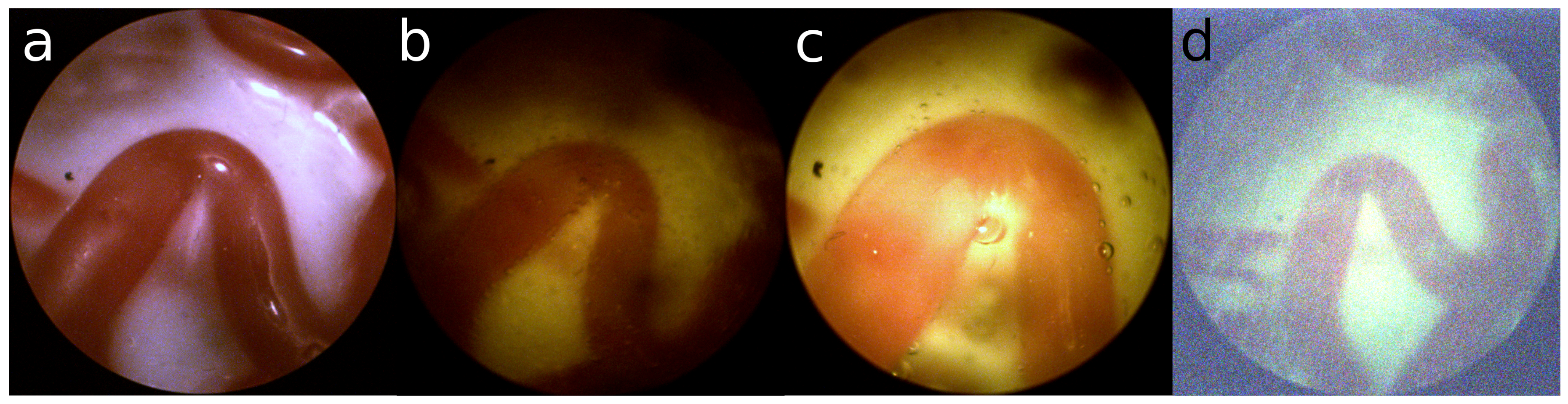
Figure 2.
Ex-vivo: (a) sufficient structure; In-vivo: (b) nominal; (c) close and bright; (d) far and dark.
Figure 2.
Ex-vivo: (a) sufficient structure; In-vivo: (b) nominal; (c) close and bright; (d) far and dark.

Figure 3.
Constraints on (a) edge; (b) circular; (c) curve; (d) veins.

Figure 4.
(a) Definition of Bounding Box (BBox); (b) Definition of Rotated Box (RBox).

Figure 5.
(a) Sample image; (b) annotated center line; (c) selection of annotated RBoxes.

Figure 6.
(a) Left: Detection network architecture; (b) Right: Architecture of a single detection scale.
Figure 6.
(a) Left: Detection network architecture; (b) Right: Architecture of a single detection scale.
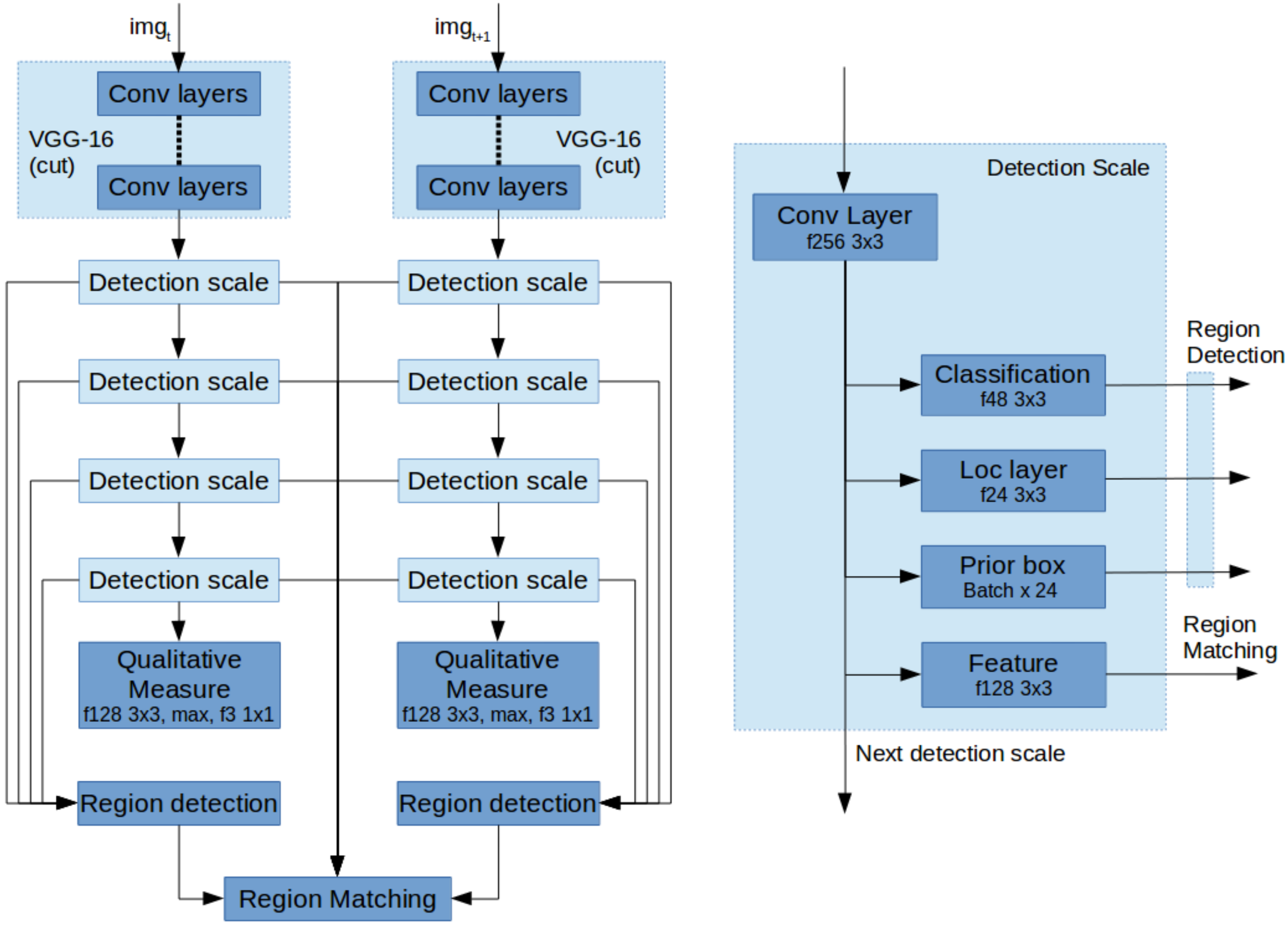
Table 1.
Number of detections and precision.
| Threshold | Ex-Vivo | In-Vivo | ||
|---|---|---|---|---|
| BBox | RBox | BBox | RBox | |
| 0.95 | ||||
| 0.90 | ||||
| 0.80 | ||||
| 0.70 | ||||
| 0.60 | ||||
Table 2.
Qualitative Measure Precision.
| Measure | Variation | Ex-Vivo | Yellow | Green |
|---|---|---|---|---|
| Distance | close | |||
| nominal | ||||
| far | ||||
| Illumination | dark | |||
| nominal | ||||
| light | ||||
| Matching | ||||
| Registration | ||||
© 2018 by the authors. Licensee MDPI, Basel, Switzerland. This article is an open access article distributed under the terms and conditions of the Creative Commons Attribution (CC BY) license (http://creativecommons.org/licenses/by/4.0/).
Share and Cite
MDPI and ACS Style
Gaisser, F.; Peeters, S.H.P.; Lenseigne, B.A.J.; Jonker, P.P.; Oepkes, D. Stable Image Registration for In-Vivo Fetoscopic Panorama Reconstruction. J. Imaging 2018, 4, 24. https://doi.org/10.3390/jimaging4010024
AMA Style
Gaisser F, Peeters SHP, Lenseigne BAJ, Jonker PP, Oepkes D. Stable Image Registration for In-Vivo Fetoscopic Panorama Reconstruction. Journal of Imaging. 2018; 4(1):24. https://doi.org/10.3390/jimaging4010024
Chicago/Turabian StyleGaisser, Floris, Suzanne H. P. Peeters, Boris A. J. Lenseigne, Pieter P. Jonker, and Dick Oepkes. 2018. "Stable Image Registration for In-Vivo Fetoscopic Panorama Reconstruction" Journal of Imaging 4, no. 1: 24. https://doi.org/10.3390/jimaging4010024
Note that from the first issue of 2016, this journal uses article numbers instead of page numbers. See further details here.